Data–Driven Fault Diagnosis of a Wind Farm Benchmark Model


1
Dipartimento di Ingegneria, Università degli Studi di Ferrara, Via Saragat 1E, 44122 Ferrara (FE), Italy
2
Dipartimento di Ingegneria dell’Energia Elettrica e dell’Informazione “Guglielmo Marconi”—DEI, Alma Mater Studiorum Università di Bologna, Viale Risorgimento 2, 40136 Bologna (BO), Italy
*
Author to whom correspondence should be addressed.
Energies 2017, 10(7), 866; https://doi.org/10.3390/en10070866
Submission received: 28 April 2017
/
Revised: 16 June 2017
/
Accepted: 25 June 2017
/
Published: 28 June 2017
(This article belongs to the Special Issue Wind Turbine 2017)
Abstract
:The fault diagnosis of wind farms has been proven to be a challenging task, and motivates the research activities carried out through this work. Therefore, this paper deals with the fault diagnosis of a wind park benchmark model, and it considers viable solutions to the problem of earlier fault detection and isolation. The design of the fault indicator involves data-driven approaches, as they can represent effective tools for coping with poor analytical knowledge of the system dynamics, noise, uncertainty, and disturbances. In particular, the proposed data-driven solutions rely on fuzzy models and neural networks that are used to describe the strongly nonlinear relationships between measurement and faults. The chosen architectures rely on nonlinear autoregressive with exogenous input models, as they can represent the dynamic evolution of the system over time. The developed fault diagnosis schemes are tested by means of a high-fidelity benchmark model that simulates the normal and the faulty behaviour of a wind farm installation. The achieved performances are also compared with those of a model-based approach relying on nonlinear differential geometry tools. Finally, a Monte-Carlo analysis validates the robustness and reliability of the proposed solutions against typical parameter uncertainties and disturbances.
1. Introduction
The increased level of wind-generated energy in power grids worldwide raises the levels of reliability and sustainability required of wind turbines. Wind farms should have the capability to generate the desired value of electrical power continuously, depending on the actual wind speed level and on the grid demand.
As a consequence, the possible faults affecting the system have to be properly identified and treated, before they endanger the correct functioning of the turbines or become failures. Megawatt-sized wind turbines are extremely expensive systems, and therefore their availability and reliability must be high in order to assure the maximisation of the generated power while minimising the operation and maintenance (O & M) services. Alongside the fixed costs of the produced energy (mainly due to the installation and the foundation of the wind turbine), the O & M costs could increase the total energy cost by up to about 30%, particularly considering offshore installation [1].
These considerations motivate the introduction of fault diagnosis systems that can also be coupled with fault-tolerant controllers [2,3]. Actually, most of the turbines feature a simply conservative approach against faults that consists of the shutdown of the system to wait for maintenance service. Hence, effective strategies to cope with faults must be studied and developed for improving the turbine performance, particularly in faulty working conditions. Their benefits would concern the prevention of failures that jeopardise wind turbine components, thus avoiding unplanned replacement of functional parts, as well as the reduction of the O & M costs and the increment of the energy production. The advent of computerised control, communication networks, and information techniques brings interesting challenges concerning the development of novel fault detection and diagnosis (FDD) and fault-tolerant control (FTC) design strategies for industrial processes.
Indeed, in recent years, many contributions have been proposed related to the topics of fault diagnosis of wind turbines and wind farms (e.g., [4,5]). Some of them highlight the difficulties in achieving the diagnosis of particular faults (e.g., those affecting the drive-train) at the wind turbine level. However, these fault are better dealt with at the wind farm level, when the wind turbine is considered in comparison to other wind turbines of the wind farm [2]. Moreover, fault-tolerant control of wind turbines has been investigated e.g., in [3,6] and international competitions on these issues arose [7,8].
The benchmark model for the wind farm fault detection and isolation (FDI) that is considered in this work was previously proposed in [2]. Based on this model, an international competition on wind farm FDI was also organised. Selected contributions were presented at the International Federation of Automatic Control (IFAC) World Congress 2014, and the three top solutions for this competition were considered and evaluated in [8]. These three works were proposed by Borchersen et al. [9], Blesa et al. [10], and Simani et al. [11]. In particular, the FDI system designed in [9] takes advantage of the fact that several of the turbines within a wind farm will be operating under similar conditions. To enable this, the turbines are grouped into several groups of similar turbines, then the turbines within each group are used to generate residuals for the turbines in the group. The generated residuals are then evaluated using dynamical cumulative sum (CUSUM). On the other hand, [10] addressed the FDI problem for the wind farm using interval parity equations (IPE). Fault detection is based on the use of parity equations and unknown but bounded description of the noise and modelling errors. The fault detection test is based on checking the consistency between the measurements and the model by finding if the formers are inside the interval prediction bounds. The fault isolation algorithm analyses the observed fault signatures on-line, and matches them with the theoretical ones obtained using structural analysis. Finally, the same authors in [11] proposed an FDI solution relying on fuzzy residual generators that are identified from the noisy measurements acquired from a simulated wind park. Note, however, that these fuzzy residual generators did not generate the reconstruction of the fault functions, as proposed in this work. Therefore, the fault diagnosis of wind turbine and wind farm systems has been proven to be a challenging task, and motivates the research activities carried out through this paper.
In recent years, the increasing demand for energy generation from renewable sources has led to a growing attention on wind turbines. Indeed, they represent very complex systems which require reliability, availability, maintainability, safety, and, above all, efficiency in the generation of electrical power. Thus, new research challenges arise—in particular in the context of modelling and control. Advanced control systems can also provide the optimisation of energy conversion and guarantee the desired performances, even in the presence of possible anomalous working conditions caused by unexpected faults.
This work deals with the fault diagnosis of a wind farm system, and it proposes the application of viable and reliable solutions to the problem of earlier fault detection, isolation, and estimation. Further, fault-tolerant controllers (which are not considered in this work) can be based on the fault diagnosis module developed in this paper, which provides the on-line information on the faulty or fault-free status of the system and the fault estimation, so that the controller action can be compensated. The design of the fault diagnosis system involves data-driven approaches, as they offer an effective tool for coping with a poor analytical knowledge of the system dynamics, noise, uncertainty, and disturbance.
The first data-driven proposed solution relies on fuzzy Takagi–Sugeno models, which are derived from a clustering c-means algorithm, followed by an identification procedure solving the noise-rejection problem. Furthermore, a second solution makes use of neural networks to describe the strongly nonlinear relationships between measurement and faults. The chosen network architecture belongs to the nonlinear autoregressive with exogenous (NN-NARX) input topology, as it can represent a dynamic evolution of the system over time. The training of the neural network fault estimators exploits the classic back-propagation Levenberg–Marquardt algorithm, which processes a set of acquired target data.
A purely nonlinear model-based scheme for fault-tolerant control purposes was also proposed by the same authors in [12], which is based on nonlinear differential geometric approach (NLGA) tools [13]. Already suggested by the authors also in the aerospace framework [14], it was extended by the same authors to the active fault-tolerant control for the same wind farm simulator [12], but it is considered here only for comparison purposes.
The developed fault diagnosis schemes are tested by means of a high-fidelity benchmark model that simulates the normal and the faulty behaviour of the wind farm system. The performances achieved via the data-driven approaches are analysed and compared with the proposed nonlinear model-based approach. Moreover, a Monte-Carlo analysis validates the robustness and reliability features of the proposed fault diagnosis schemes against the typical parameter uncertainties and disturbances. Finally, the effectiveness shown by the obtained results suggests further investigations of the industrial application of the proposed fault diagnosis methodologies.
It is worth highlighting the key features of the proposed fault diagnosis strategies. First, the proposed methodologies relying on fault estimators used as residuals represent one novel aspect of the suggested FDI/FDD strategies. These estimations are achieved using both neural networks and fuzzy systems. On one hand, even if neural networks estimators are well-known and well-established for fault classification and fault detection, they are used here for the reconstruction of the fault function. On the other hand, the performances of these neural estimators are compared with the fuzzy estimators which are based on the parameter estimation methodology suitably developed by the same authors in [15]. Additionally, in this case, this fuzzy strategy was already proposed by the same authors for fault-tolerant control purposes by means of both active and passive schemes (e.g., [12]); however, these tools are exploited in this work for the first time for solving the FDI/FDD tasks applied to the wind farm benchmark, and using the fault reconstruction principle. Moreover, it is quite well established that FDI methods relying on fault estimation strategies rather than classical residual generation techniques result to be more robust (e.g., [16]). Moreover, the final comparisons among the data-/driven and model-based FDD approaches are indeed very meaningful. In fact, the fuzzy approach relies on the errors-in-variables (EIV) framework, whilst the neural network approach considers equation error models (NN-NARX). On the other hand, these two data-driven schemes are compared with a purely nonlinear methodology that exploits a model-based disturbance decoupling method (the NLGA adaptive filters). These FDD schemes are compared for the first time when applied to a wind farm simulator.
The work is organised as follows. Section 2 recalls the wind farm benchmark simulator. Section 3 describes the FDD schemes for residual generation relying on fuzzy prototypes and neural network structures. A purely nonlinear approach proposed by the authors for wind turbine FDD is summarised in Section 4. The achieved results are reported in Section 5. Comparisons with the recalled model-based nonlinear FDD strategy are also reported. Finally, Section 6 concludes the paper by summarising the main achievements of the work, and providing some suggestions for further research issues.
2. Wind Farm Benchmark Model
The wind farm benchmark model considered in this work has been proposed in [2] by the same authors who developed the wind turbine benchmark model [3].
It consists of nine wind turbines arranged in a squared grid of three rows and three columns. The complete wind farm model consists of three main submodels: the wind and wake model, the plant model, and the controller model, interacting as sketched in Figure 1.
Two measuring masts are located in front of the wind turbines, one in each of the wind directions considered in this benchmark model (e.g., and ). The wind speed is measured by these measuring masts which are located at a distance of 10 times L in front of the wind farm. In this way, the measuring devices are not affected by the wind turbine wakes, and are able to provide sufficiently accurate wind speed measurements.
The farm uses generic MW wind turbines, which are three-bladed horizontal-axis, pitch-controlled, variable-speed wind turbines. Each of the wind turbines is described by simplified models including control logics, variable parameters, and three states.
The wind and wake models provide the wind speed for each of the nine turbines, contained in the vector , as well as for a measuring mast . They are determined starting from a certain wind sequence (two different wind sequences are included in the simulator), and their elaboration takes into account the delay and the interaction among the turbines depending on wind direction. In particular, the wake effect is described as reported in [17] by means of a static deficit coefficient of . Finally, the turbulence is modelled by an additive Gaussian white noise.
The overall plant model represents the nine wind turbines with the same submodel for each of them. It receives as input the vector and the vector containing the nine reference signals from the controller. The outputs are the vectors , , that contain the generated powers, the pitch angles, and the generator speeds, respectively, for each of the nine turbines [3]. Inside the wind turbine submodels, the current wind speed is suitably elaborated in order to compute the available power and the generated power [2].
Finally, the wind farm controller forces each turbine to follow a reference power signal that is of the wind farm power reference. More details regarding the wind farm benchmark simulator can be found in [2].
2.1. Wind Farm Fault Scenario and Model Parameters
Three common fault scenarios are considered [2]; they affect the output variables of the plant system. These kinds of faults are difficult to detect considering a single wind turbine, but they can be identified at the wind farm level.
The first fault considered represents the debris build-up on the blade surface. Its effect corresponds to a change of the aerodynamics of the affected turbine and the consequent decreasing of the generated power that is modelled by a scaling factor of applied to the generated power signal. An analysis of this kind of fault is reported in [18].
The second fault is a misalignment of one blade caused by an imperfect installation. The effect is an offset between the actual and the measured pitch angle of the affected turbine. This fault can excite structural modes and creates undesired vibrations that can damage the system severely. The faulty signal involves an offset of on the pitch angle.
The third fault represents the wear and tear in the drive-train. It was demonstrated [7] that this kind of fault is difficult to detect at the wind turbine level, and the current trend is to analyse the frequency spectra of different vibration measurements. In this benchmark model, the fault affects the generated power, increasing the amplitude of its oscillation by 26% of the nominal value, and the generator speed increasing the amplitude of its oscillation by 130%.
Table 1 summarises the considered faults with a brief description of their typology and topology, with respect to their causes and effects, which will be exploited for the fault sensitivity analysis proposed in Section 3.2.
Finally, Table 2 reports the parameters used in the wind farm benchmark model.
3. Data-Driven Fault Diagnosis Strategies
This section introduces the fault diagnosis schemes adopted in the simulations summarised in Section 5. Firstly, the fault diagnosis strategy is described in Section 3.1, followed by the summary of the design of the suggested data–driven residual generation methodologies relying on fuzzy prototypes and neural networks recalled in Section 3.3 and Section 3.4, respectively.
3.1. Fault Diagnosis Scheme
In the following the discrete-time monitored systems (i.e., the faults on the input and output measurements that are acquired from the wind farm simulator, as represented in Figure 2), are described in the form of Equation (1):
where and are the actual unmeasurable variables, whilst and represent the sensor measurements affected by both the measurement noise and the faults. and are additive fault signals, which assume values different from zero only in the presence of faults. Note that these terms represent equivalent fault signals that produce the same effects of the actual faults affecting the wind farm, as described in Section 2.1.
According to the EIV framework, the unmeasurable inputs and outputs and represent the physical variables that are measured by means of input and output sensors, as depicted in Figure 2.
The same considerations hold for the measurement noise or error signals and . They are modelled as white Gaussian process additive noise terms on the actual measurements acquired from the process under investigation, and are equivalent signals representing the actual effect of the measurement errors. This representation is also known as the errors-in-variables (EIV) model [19].
Figure 2 shows the general scheme with the faults affecting the system under diagnosis (i.e., the wind farm) as equivalent additive signals on the input and output measurements (sensors).
Among the different approaches to generating the residual signals available in the related literature, the solution proposed in this work exploits two approaches. They rely on fuzzy and neural network models, which provide on-line estimations of the fault signals and . Hence, as shown in Figure 3, the residuals are represented by the estimated fault signals generated by the fault estimators filtering the measured (sampled) inputs and outputs and , respectively:
The generic i-th signal of the vector represents one of the components of the faults and affecting one of the input or output measurement sensors. This equivalent signal representation is used to model the actual faults of the wind farm described in Section 2.1.
Figure 3 sketches the residual generation scheme that is achieved via the fault estimator system by using the acquired input and output measurements and . The fault diagnosis process requires the FDI tasks as a first step. As the residual is equal to the estimated fault signal, it is easily performed here by using a proper thresholding logic directly operating on the residuals, without requiring their elaboration with any evaluation functions, as addressed for example in [16].
Therefore, the occurrence of the i-th fault can be simply detected via the threshold logic of Equation (3) applied to the i-th residual :
where the i-th component of the residual vector of Equation (2) is considered a random variable whose unknown mean and variance are estimated in fault-free condition after the acquisition of N samples, as shown by the relations of Equation (4):
The tolerance parameter has to be properly tuned in order to separate the fault-free from the faulty situations. The value determines the trade-off between the false alarm rate and the fault detection probability. A common choice of can rely on the three-sigma rule; otherwise, extensive simulations can be performed to optimise the value. Note that the three-sigma rule represents a rule of thumb, according to which, in certain problems of probability theory and mathematical statistics, an event is considered to be practically impossible if it lies in the region of values of the normal distribution of a random variable at a distance from its mathematical expectation of more than three times the standard deviation. Therefore, assuming that the probability distribution function of the diagnostic residuals is normally distributed, mean value and standard deviation , the probability that these residual signals lies in the range between and assumes the value of . This rule easily allows for the FDI, while minimising the false alarm and the missed fault rates, and at the same time maximising the correct FDI rate, for a suitable number of values of .
As a consequence of the fault detection, the fault isolation task is easily achieved by means of a bank of estimators. As described by Equation (1), the faults are considered as equivalent signals that affect the input measurements (i.e., ) or the output measurements ().
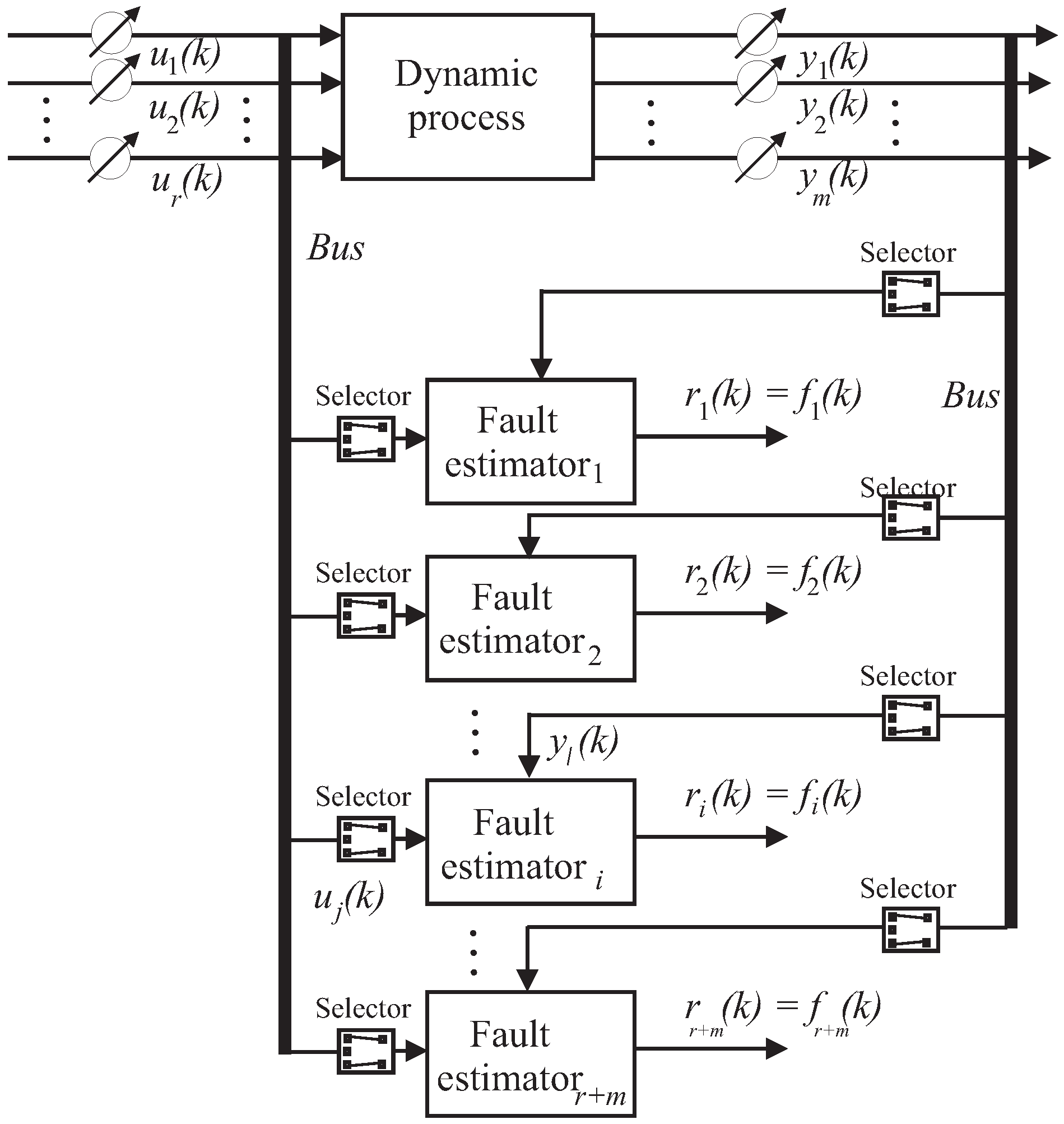
Under these assumptions, by following the scheme of the generalised estimator configuration of Figure 4, in order to uniquely isolate one of the input or output faults, by considering that multiple faults cannot occur, a bank of multi-input single-output (MISO) fault estimators is used. In general, the number of these estimators is equal to the number of faults that have to be diagnosed; i.e., in general equal to the number of input and output measurements, . Therefore, in general the i-th fault estimator that reconstructs the fault should be driven by the components of the input and output signals and that are sensitive to the specific fault . Therefore, it should be clear that the design of these fault estimators is enhanced by the fault sensitivity analysis described in Section 3.2. For each fault case, its resulting effects on the rest of the system are analysed, and in particular the most sensitive input and output measurements to that specific fault situation are identified. In this way, by means of the fuzzy system and neural network tools, it will be possible to derive the dynamic relationships between the input–output measurements and the faults, as represented by the estimator bank of Figure 4.
Figure 4 shows this generalised fault estimator scheme, where the fault estimators are driven only by the input–output signals selected via the fault sensitivity tool addressed in Section 3.2, so that the relative residual is insensitive only to the fault affecting those inputs and outputs defined by the selector blocks. It is worth noting that multiple faults occurring at the same time could be correctly isolated using this configuration if the fault sensitivity procedure is properly performed.
The capabilities of the adopted estimator bank can be summarised by means of the so-called fault signature matrix depicted in Table 3, where each entry that is characterised by a value equal to “1” means that the considered residual (i.e., the equivalent fault) is sensitive to the actual fault effect (“0” otherwise), under the hypothesis mentioned above. Note that the total number of equivalent fault signals is equal to the number of input and output measurements, i.e., .
As already remarked, the fault sensitivity analysis that has to be executed before the design of the fault estimators suggests how to select the input–output configuration for the fault estimator bank. This input–output selection procedure, (which is briefly remarked here) will be addressed in more detail in Section 3.2. Then, the design of the fuzzy or neural network models can be performed, as recalled in Section 3.3 and Section 3.4, respectively. Finally, the fault estimate (residual) threshold test logic of Equation (3) allows the achievement of the fault diagnosis tasks.
Therefore, the residual analysis proposed in Section 3.2 enhances the design of the fault estimator bank configuration described in this section.
3.2. Fault Sensitivity Analysis for the Wind Farm System
This fault sensitivity analysis has been performed on the wind farm simulator. This tool represents an analysis aimed at determining the most sensitive measurements with respect to the simulated fault conditions. In practice, the assumed fault signals have been injected into the benchmark simulator, assuming that only a single fault may occur in the considered plant. Then, the relative mean square errors (RMSEs) between the fault-free and faulty measured signals are computed, so that for each fault , the most sensitive signals ( and ) to that specific fault are selected.
In particular, this analysis is conducted on the basis of a selection algorithm that is achieved by introducing the normalised sensitivity function , defined in the form of Equation (5):
where:
Its value represents the effect of the considered fault case with respect to a certain measured signal . The subscripts “f” and “n” indicate the faulty and the fault-free case, respectively. Therefore, the measurements mostly affected by the considered fault imply a value of equal to “1”. Otherwise, smaller values of mean that the signal x is not practically affected by the fault. The signals characterised by the highest value of can be selected as the most sensitive measurements, and they will be considered in the design of the fault diagnosis blocks.
The results of this sensitivity analysis are reported in Table 4 for the wind farm benchmark. The selected signals for each fault included in the wind farm benchmark are divided as inputs and outputs.
As a result, the fault diagnosis blocks that are designed as shown in Figure 4 exploit the reduced subset of input and output signals and of Table 4, instead of using all the system measurements recalled in Section 2. Moreover, this leads to a noteworthy simplification of the residual generator structure, thus also providing a decrease in the computational effort. The estimated fault (residual) threshold test logic of Equation (3) leads to the achievement of the fault diagnosis task. The design of the fuzzy systems and neural networks will be recalled in the next Section 3.3 and Section 3.4, respectively.
Finally, it is worth noting that this sensitivity analysis can be considered a stage of the so-called failure mode and effect analysis (FMEA) [20] which was already performed on this benchmark, as described in Section 2.1, where the fault scenario and the effects on the system behaviour were summarised. Indeed, this section is focused on a further sensitivity analysis. This means that the fault causes described in Section 2.1 are modelled as equivalent input and output signals affecting the input and output measurements and , respectively. In this way, the fault sensitivity analysis is achieved in order to determine the most sensitive input–output measurements to these equivalent fault causes. These most sensitive measurements to faults describe the effects of the faults themselves. Afterwards, these signals are used to design the banks exploited for both the fault reconstruction and the fault isolation tasks addressed in Section 3.4.1.
3.3. Fuzzy System Modelling
This section describes the design of the fault estimators that is achieved by means of Takagi–Sugeno (TS) prototypes [21]. Indeed, the unknown relationships between the measurements acquired from the wind farm simulator and the considered faults are described by fuzzy models. They consist of a number of rules connecting the inputs with the output of the system under diagnosis, on the basis of a knowledge of its dynamics in form of IF ⟹ THEN relations, processed by fuzzy reasoning [22].
The approximation of nonlinear multi-input single-output (MISO) systems (but also extension to MIMO—multiple-input multiple-output—systems can be considered) is achieved by the TS fuzzy reasoning, as reported, for example, in [23,24]. According to the TS modelling approach, the consequents become crisp functions of the input, while the antecedents remain fuzzy propositions; therefore, the fuzzy rule takes the form of Equation (8) [21]:
where i indicates the number of rules, with . The antecedent does not differ from the Mamdani rules, with a combined membership function that considers the logical connectives expressed by linguistic propositions. The rule consequent functions have a defined structure: it is the instance of parametrised function in affine form:
where is a parameter vector and is a scalar offset, while is the i-th rule output. The number of rules is supposedly equal to the number of clusters used for partitioning the data into regions where local affine relations can be assumed [22]. Furthermore, the antecedent of each rule defines the degree of fulfilment for the corresponding consequent model, so that the rule global model can be seen as a fuzzy composition of local affine models.
Thus, the TS inference takes the form of the simple algebraic expression of Equation (10):
According to this description, the estimated fault is the weighted average of affine functions of the measured input and output signals, where the weights are the combined degree of fulfilment of the system input and output measurements and .
It is worth noting that the nonlinear system under diagnosis has a dynamic behaviour; therefore, the considered model input vector can contain the current as well as the previous samples of the process input and output measurements and .
Indeed, in order to introduce the time dependence into the model of Equation (8), the consequents are considered as discrete-time linear autoregressive models with exogenous input (ARX) of order o, in which the regressor vector takes the form of Equation (11):
where and are the actual system input and output vectors, whose subscript indices and depend on the fault sensitivity selection procedure of Section 3.2, with and , where r is the number of inputs and m the number of outputs . k is the time step, with . The affine parameters of Equation (9) can be grouped as in the expression of Equation (12):
where the coefficients are associated to the output samples, and the are associated to the input samples.
An effective approach to the design of a fuzzy inference system (FIS) as approximator of a complex nonlinear system begins with the partitioning of the available data into subsets characterised by simpler (affine) behaviour. A cluster can be defined as a group of data that are more similar to each other rather than to the members of another cluster. The similarity among data can be expressed in terms of their distance from a particular item, exploited as the cluster prototype. Fuzzy clustering provides an effective tool to obtain a partitioning of data in which the transitions among subsets are smooth, rather than abrupt.
Indeed, fuzzy clustering allows an item to belong to several clusters simultaneously, with different degrees of fulfilment, whereas the classic crisp clustering relies on mutually exclusive subsets. Different clustering methods have been proposed in the literature; see e.g., the review [25], or more recent works [26,27].
Typically, the available data consist of noisy measurements acquired from the system under diagnosis. They are grouped into the data matrix , whose columns are the vectors z containing the measurements of a single observation of the monitored process:
where n is the data dimension, and N is the number of available observations.
Most fuzzy clustering algorithms are based on the optimisation of the c-means goal function performed as follows:
- the data matrix of Equation (13) is defined;
- the so-called fuzzy partition matrix is defined, which contains the values of the membership function for the couple i-th measurement/k-th cluster;
- the vector containing the cluster prototypes is defined; they have to be determined and represent the centres from which the distance of each measurement is computed.
The widespread c-means goal function adopted in this work was formulated in [28] and is defined in the form of Equation (14):
being the weighting exponent, and:
the squared inner product distance norm, with and . The matrix determines the cluster shape.
The minimisation algorithm exploits a series of Picard’s iterations that updates the cluster prototypes and of the partition matrix , until a stop criterion is met [22]. Note that in numerical analysis, fixed-point iteration is a method of computing fixed points of iterated functions. Solving a problem in this way is called Picard iteration, Picard’s method, or the Picard iterative process.
An important point concerns the determination of the optimal number of clusters , since the clustering algorithm assumes a suitable number of clusters, regardless of whether or not they are actually present in the data. Once the partition matrix has been estimated, the antecedent degrees of fulfilment in are easily estimated by interpolation or curve fitting methods [22].
3.3.1. Fuzzy Model Parameter Estimation
After the determination of and , the design of the FIS can be considered as system identification problem since it requires the estimation of the consequent parameters and of Equation (9) in a noisy environment. The identification scheme adopted in this work was proposed by the same authors in [15] and successfully exploited in the approximation of nonlinear functions through the piecewise affine models (as shown, e.g., in [19]). This approach is based on the minimisation of the prediction errors of the individual TS local models considered as independent problems. Moreover, their solutions rely on the so-called Frisch scheme [29] that is usually exploited in connection with the identification EIV models [19]. This assumption is motivated by the relations of Equation (1), where the input and output measurements are affected by both noise and fault effects.
In fact, the discrete-time dynamic model already represented in Figure 2 is considered in the EIV framework; the noise is supposed to affect the inputs as well as the output measurements as additive signals and on the noise-free unmeasurable quantities and , in the form of Equation (16):
Therefore, by considering the i-th TS consequent of the type of Equation (10) and the associated local ARX model of order o with the regressors grouped into the vector as in Equation (11), the acquisition of noisy measurement of input and output samples collected into the vector permits the construction of the i-th data matrix defined as:
with reference to the generic fault signal . The i-th covariance matrix from the acquired data can be computed as:
that is a positive-definite matrix consisting of the sum of two terms:
where refers to the noise free signals, while is the noise covariance matrix, which depends on the unknown noise variances and through the expression:
The solution of the identification problem mentioned above requires the estimation of and , which can be performed solving the expression in the form of Equation (21):
with:
in the unknown variables and .
In case all the assumptions regarding the Frisch scheme [15] are satisfied, there exists one common point belonging to all the surfaces determined as the root locus of Equation (21), which represents the actual noise variance values . However, in real cases, the Frisch assumptions are commonly violated, so a unique solution cannot be obtained. In these situations, the identification aims at finding the nearest point of all the surfaces. More details regarding this issue can be found, e.g., in [19,29].
After the computation of the variances, the covariance noise matrix can be built as in Equation (20), and the linear parameters in each cluster (therefore in each TS consequent) can be finally determined as a solution of the following expression:
3.4. Neural Network Modelling
Alongside the fuzzy models, a different data-driven approach based on neural networks, has been proposed in order to implement the fault diagnosis block for estimating the generic fault signal . In this section, after a brief introduction on the general structure, the properties, functioning, and architecture of a neural network are recalled. They will be exploited to implement the neural network fault estimators of Figure 4.
In this work, a set of neural network estimators is designed and trained in order to reproduce the behaviour of the faults affecting the system under investigation, thus accomplishing the modelling and identification task. The structure of the i-th single neuron [30] is also called a perceptron. It features a MISO system where the output is computed as a function f of the weighted sum of all the neuron inputs , with the associated weights . The function f—called the activation function—represents the engine of the neuron.
A structural categorisation of neural networks concerns the way in which their elements are connected to each other [31]. In a feed-forward network (also called multilayer perceptron), neurons are grouped into unidirectional layers.
On the other hand, recurrent networks [32] are multilayer networks in which the output of some neurons is fed back to neurons belonging to previous layers, and thus the information flows in forward as well as in backward directions, allowing a dynamic memory inside the network.
A noteworthy intermediate solution is provided by the multilayer perceptron with a tapped delay line, which is a feed-forward network whose inputs come from a delay line. This kind of network represents a suitable tool to model or predict unknown functions. In particular, the NN-NARX belongs to this latter category, as its inputs are delayed samples of the system inputs and outputs. Indeed, if properly trained, a NN-NARX can reconstruct an unknown function with arbitrary accuracy on the basis of the acquired past measurements of system inputs and outputs.
Generally speaking, considering a MISO system, the elaborations of the NN-NARX follow the law described by the relation of Equation (24):
where is the estimation of the generic i-th fault, whilst and are the -th and -th measured system inputs and outputs, respectively, properly selected according to the fault sensitivity procedure of Section 3.2, with and , where r is the number of inputs and m the number of outputs , . k is the time step, whilst and are the number of delays for the input and the output signals, respectively. is the function realized by the network, which depends on the layer architecture, the number of neurons, their weights, and their activation functions. The general fault estimation task of this NN-NARX used as fault estimator for fault diagnosis is depicted in Figure 5.
The design parameters of the overall architecture are represented by its number of neurons and the connections between layers, whilst the values of the weights inside each neuron are derived from the neural network training algorithm.
A NN-NARX is a learning system requiring an initial training procedure that adjusts the weights to improve the network performance. When the network task is the estimation of a nonlinear function, the training is performed by presenting a set of examples of proper behaviour to the network, consisting of the inputs and (patterns), and the desired output (target) for the relative inputs.
The training phase objective is the minimisation of a performance function E, which depends on the weight vector .
Generally speaking, considering a number P of available example patterns consisting of the input–target pairs (, ), with , defining the output generated by the network fed by , the p-th error vector can be expressed as:
with , and m the general number of outputs of the neural network. Furthermore, the overall error vector collects each :
Consequently, the performance function becomes:
where the dependence of E by the N parameters grouped in the vector is implicit in the generated output .
Standard numerical optimisation algorithms can be used to update the parameters, in order to minimise E. Among these, the most common are iterative, and make use of characteristic matrices such as the gradient (or the Hessian ) of the performance function, or the Jacobian of the estimation error. These training algorithms update the parameters of the neural network until a stop criterion is met and use the updating rules of the most common optimisation algorithms (i.e., the gradient descent, the Newton, the Gauss–Newton, and the Levenberg–Marquardt algorithm) [33].
Finally, as shown in Section 5, the neural network fault estimator blocks have been trained exploiting the Levenberg–Marquardt method [34], which uses the back-propagation training technique.
3.4.1. Fault Diagnosis Design Procedure
The complete design flow relying on both fuzzy systems and neural networks used as fault estimators for fault diagnosis is summarised in Figure 6.
Note that the schemes summarised in Figure 6 highlight some similarities between the fuzzy system and the neural network prototypes. The logic schemes of Figure 6 aim only at showing the general procedure used for the design of the fault diagnosis schemes, which are based on both the neural networks and the fuzzy models. Moreover, common steps exploited in both the neural network and fuzzy model fault diagnosis system design are shown.
Finally, it is worth noting that the design flow sketched in Figure 6 assumes that only single faults affect the process under diagnosis. However, the structure of the fault estimator bank shown in Table 3, and the input selection procedure highlighted in Section 3.2 allows the isolation of multiple and simultaneous faults.
4. Model-Based Fault Diagnosis Method
This section recalls the purely nonlinear fault diagnosis scheme that represents a model-based approach mainly used for comparison purposes, as summarised in Section 5. In particular, this method is based on analytical physical law modelling and partially on the parameter estimation of some coefficients describing this mathematical relation.
The proposed fault diagnosis scheme consists of three phases. The first step regards the estimation of the nonlinear disturbance distribution functions, which are required for the design of the nonlinear adaptive filter for fault estimation. The fault reconstruction is thus exploited for the diagnosis of faults in the measured signals.
In order to achieve a robust and effective fault diagnosis solution, the fault estimations must be decoupled from the disturbances acting on the system. Section 2 highlighted that these disturbances are represented by two effects. The first derives from the wind signal affecting the i-th wind turbine model of the wind farm through its power coefficient [2]. The decoupling of this effect was already investigated in [12], but applied to a single wind turbine. It will be used here and applied to the wind turbine models of the wind farm. The second disturbance effect is due to the interactions among the wind turbines of the wind farm, and represented by the wind wakes [2].
Solutions dealing with the first disturbance term were based on the estimation of both the wind turbine power coefficient values and the wind speed . Regarding the wind wakes, a novel strategy based on a nonlinear design scheme is proposed here. In particular, as for the decoupling of the wind speed addressed in [12], this approach requires the analytical knowledge of the nonlinear disturbance distribution relation of the unknown inputs represented by the wake effects. In more detail (as shown in [12]), the power coefficient -map appearing in the wind turbine aerodynamic models of the wind farm was estimated by means of a two-dimensional polynomial representation, which was a function of the tip-speed ratio and the blade pitch angles [35].
Once the disturbance description has been obtained in analytical form, the second stage of the fault diagnosis system design is based on the development of the nonlinear fault diagnosis filters. Their structure is obtained by exploiting a disturbance decoupling scheme belonging to the NLGA framework [36]. A coordinate transformation, highlighting a subsystem affected by the fault and decoupled by the disturbances, represents the starting point to design adaptive filters for fault estimation. By means of this NLGA approach, the fault estimate is decoupled from the disturbance d, which in this work is represented by the wake effects of the wind turbines affecting the i-th wind turbine of the wind farm.
Therefore, the proposed approach is applied to the general nonlinear model in the form of Equation (28):
where the state vector (an open subset of ), is the control input vector, is the fault, is the disturbance vector, and is the output vector. , , the columns of , and are smooth vector fields, with a smooth map.
The development of the NLGA strategy for the design of the estimator for the fault f with the decoupling of the disturbance d is based on the procedure presented in [37]. It was shown that the considered NLGA scheme extended to the fault diagnosis problem is based on a coordinate change in the state space and in the output space, such that by using the new (local) state and output coordinates , the system of Equation (28) is transformed into [37]:
with not identically zero. As remarked in [37], this procedure yields to the observable subsystem of Equation (29) that—if it exists—is affected by the faults f, and not affected by disturbances d.
This transformation can be applied to the system of Equation (28), if and only if some fault detectability conditions are satisfied [37]. The system of Equation (28) in the new reference frame is decomposed into three subsystems of Equation (29), where the first one (the so-called -subsystem) is always decoupled from the disturbances d and affected by the faults f, described in the form of Equation (30):
where—as the state in Equation (29) is assumed to be measured—the variable in Equation (30) is considered as independent input, and denoted with .
The proposed NLGA adaptive filter is based on the least-squares algorithm with forgetting factor described by the adaptation law of Equation (31):
with Equation (32) representing the output estimation, and the corresponding normalised estimation error:
where all the involved variables of the adaptive filter are scalar. In particular, is a parameter related to the bandwidth of the filter, is the forgetting factor, and is the normalisation factor of the least-squares algorithm. Moreover, the proposed adaptive filter adopts the signals , , which are obtained by means of a low-pass filtering of the signals , , as follows:
The considered adaptive filter is described by the systems of Equations (31)–(33). In [37] it was shown that this adaptive filter provides an estimation that asymptotically converges to the magnitude of the actual fault f.
This completes the design of the fault diagnosis methodology based on NLGA adaptive filters, whose results will be shown in Section 5.
5. Simulation Results
The following simulations refer to the wind farm benchmark model when the fault diagnosis schemes based on the fuzzy and neural network fault estimators are designed.
The mean wind sequence driving all the simulations covers the most common operative range from 5 m/s up to 15 m/s, with a peak value of about 23 m/s. The wind and wake submodel described in Section 2 processes this sequence in order to generate the actual wind speed signal for all the turbines of the wind farm and for both the measurement musts associated with the two wind scenarios provided by the benchmark model, as shown in Section 2, also considering the disturbances and the interaction among turbines. Figure 7 depicts the leading wind sequence.
The available data consist of 440,000 samples of input–output measurements, acquired with a sampling rate of 100 Hz.
The three proposed faults described in Section 2 affect different wind turbines at different times, by influencing the measured variables and , and in particular the signals , , related with the i-th wind turbine of the wind farm. These faults are difficult to detect at the wind turbine level. However, they can be more easily detected at the wind farm level by comparing the performance of different wind turbines. Table 5 shows the affected turbines per fault, together with the occurrence time.
These faults are simulated for the three cases of Table 1 and under the assumptions described in Section 2.1. Note that the turbines in Table 5 are also denoted by means of their row and column indices in the coordinate system, as reported in [2].
5.1. Fuzzy Estimator Results
The fuzzy fault estimators described in Section 3.3 are designed by selecting a number of clusters and delays on the input and output regressors, related to the signals selected by the fault sensitivity analysis proposed in Section 3.1. On the other hand, the optimal number of and o has been determined via extensive simulations that are exploited for minimising the cost function of Equation (14).
The TS models exploit Gaussian membership functions. Afterwards, the fault estimators are organised into a dedicated observer scheme of Section 3.1 that allows for the isolation of the three faults affecting the wind farm benchmark model described in Section 2.1.
Firstly, the capabilities of these three fuzzy fault estimators are evaluated in terms of RMSE, defined as the percent difference between the measurements and the estimation, computed in fault-free conditions. This index can be considered as the measure of the percentage of the data not correctly reconstructed by the estimator. As highlighted in Table 6, although this index increases when computed on data which are not used in the estimation phase (i.e., validation and test data sets), the percentage is always smaller than 5%, thus featuring a good modelling capability.
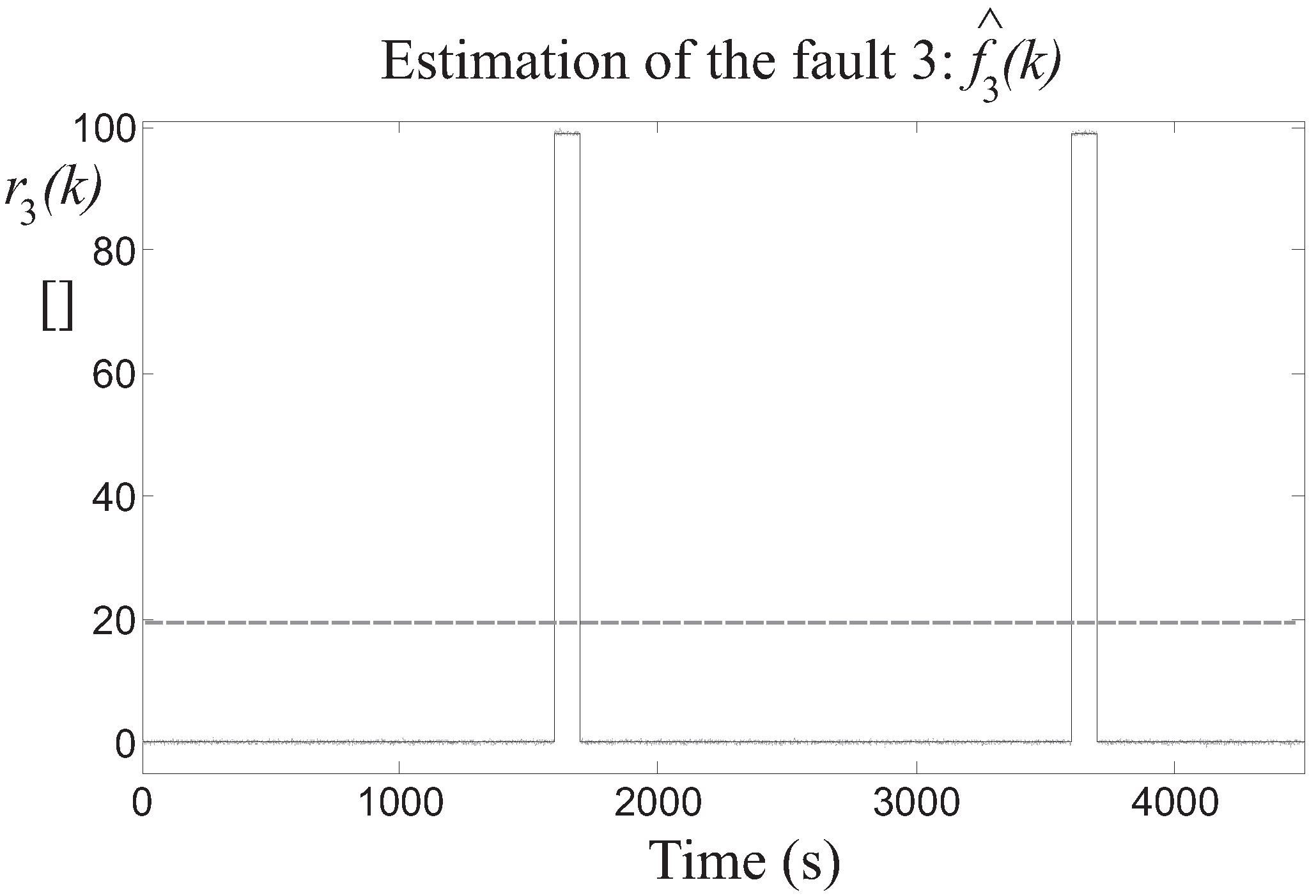
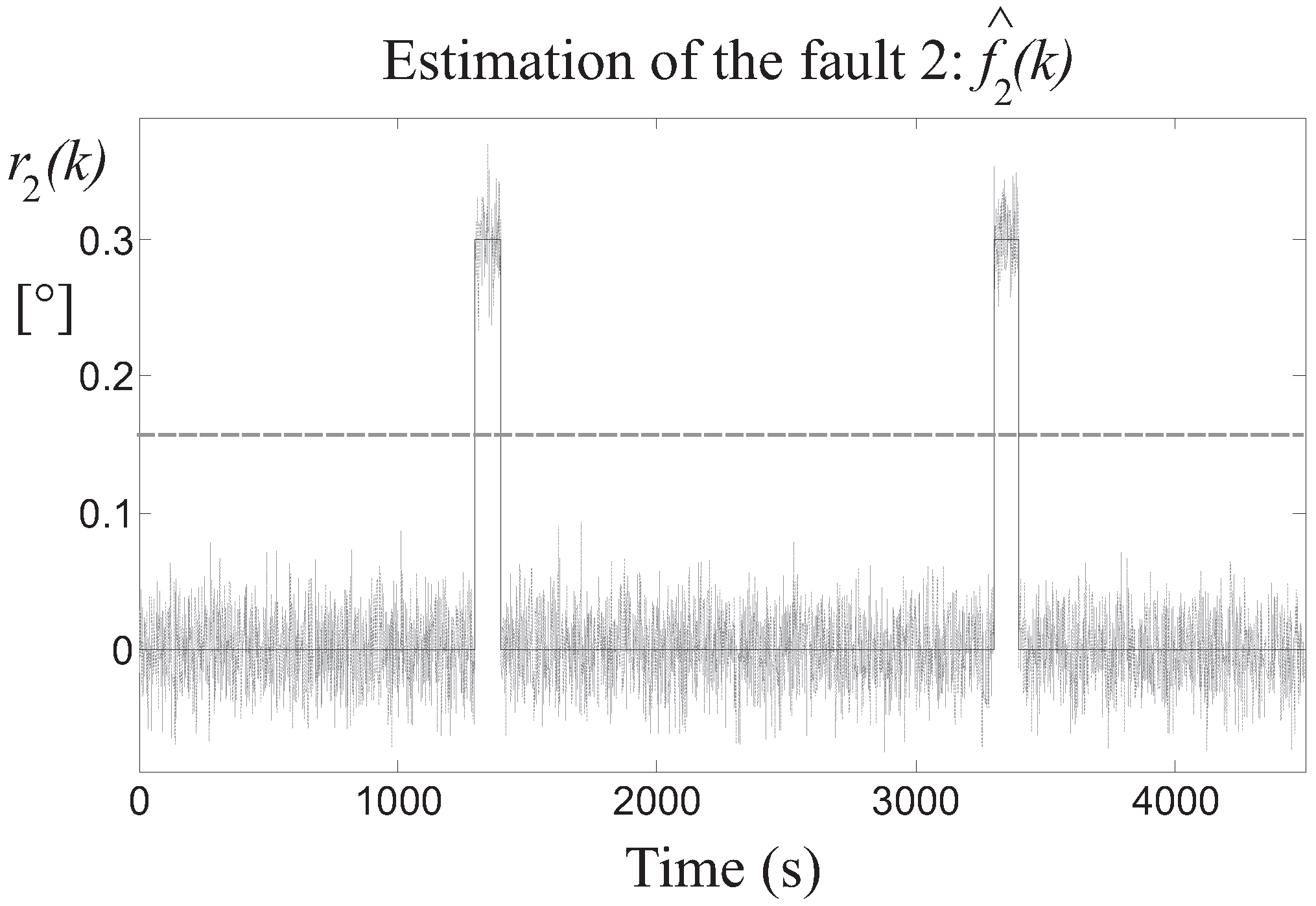
Then, the detection of the three faults is achieved by means of the residuals generated by the fault estimators, after the proper tuning of the threshold parameter . In particular, Figure 8 highlights the residual relative to the fault 1 estimator, whose value is bounded by the thresholds when the fault is not active, while it is significantly over the threshold when the fault occurs on the two different turbines. Similar results are achieved by the fault 2 and 3 estimators, whose residuals and are depicted in Figure 9 and Figure 10, respectively.
5.2. Neural Network Estimator Results
In the same way as the fuzzy estimator approach, three NN-NARX described in Section 3.4 have been designed to estimate the nonlinear behaviour between the measurements selected by the fault sensitivity analysis of Section 3.2 and the considered fault cases. The selected architecture of the networks involves three layers; namely the input, the hidden, and the output layers. The number of neurons in the hidden layer has been fixed to . The value of has been chosen for the input–output delays. Similarly to the fuzzy models, the neural networks modelling capabilities have been tested in terms of RMSE and the results are reported in Table 7 in fault-free conditions for three different data sets (training, validation, and test). Additionally, in this case, a trial and error procedure is used to determine the optimal number of the delays and , as well as the number of the neural network neurons, which leads to the minimisation of the cost function of Equation (27).
Note that three different data sets have been exploited in Table 7. In fact, in order to verify and validate the achieved results, different data sets have to be used. The wind farm benchmark is able to generate different data sequences for each simulation, as described in Section 2.
The fault detection task is achieved by comparing the residual with a fixed optimised threshold, as for the case of the fuzzy estimators, as reported in Table 8.
5.3. Fault Diagnosis NLGA Simulations
This section describes the design and the simulations of the NLGA adaptive filters applied to the wind park benchmark. In particular, the results achieved from the estimation of the disturbance terms appearing in Equation (28) are firstly presented. Once the disturbance decoupling has been achieved, the performances of the NLGA fault estimators are reported.
In more detail, the i-th -map entering into the aerodynamic model of each of the nine wind turbines of the wind farm described in Section 2 has been approximated by using a two-dimensional polynomial in the form of Equation (34):
for the i-th turbine of the wind park. More details can be found in [35]. By following the same procedure, the second disturbance term representing the function in Equation (28) is described by the polynomial representing the wind wake from the j-th turbine of the park affecting the i-th turbine:
with . In general, note that the expression of both the -map and the disturbance term in Equation (35) depend on the i-th wind turbine of the wind farm.
The suggested scheme provides the analytical description of the disturbance effects due to all uncertainties, and not only the errors due to entry changes and the wind wake interferences among the wind turbines. However, since these terms are used for the fault estimation filter design, any kind of uncertainty must be modelled. A similar approach was proposed, for example, in [16], but developed only for linear state-space models. Under these considerations, the uncertainty distribution description for the nonlinear model of Equation (28) is identified using the input–output data from the wind turbines of the wind farm. The general assumption holding for this case is that the model–reality mismatch is varying more slowly than the disturbance signals, such as d. Another important point regards the fact that the estimation aims at describing the structure of the uncertainty, which should not depend on the wind size uncertainty. Only the so-called “directions” of the disturbance represent the important effect for disturbance decoupling (i.e., the term), and not the “amplitude” of the uncertainty (i.e., the size of the disturbance d).
The designed NLGA adaptive filters of Equations (31)–(33) provide the estimate of the magnitude of the different faults acting on the the wind farm benchmark, as shown in Section 4. With reference to the overall input–affine model of the wind farm described in Section 2, the following terms can be determined:
and:
with reference to the i-th turbine, with the understanding that the subscript i is dropped. Moreover, is defined as:
If , it follows that as . On the other hand, it is necessary to compute the expression . However, for the case under investigation, the determination of the codistribution is enhanced due to the structure of Equation (40).
Finally, as an example, the design of the NLGA adaptive filter for the reconstruction of the fault case 2 is based on the expression of Equation (41):
where:
The design of the NLGA adaptive filters for the reconstruction of the faults for cases 1 and 3 is based on a different selection of the vector of Equation (38), which leads to other expressions for the filter of Equation (41). As an example, for the fault case 2 described in Section 2.1, the nonlinear filter for the reconstruction of decoupled from the disturbance d representing the effect of both the wind and the wake signals has the form of Equation (31). After a suitable choice of the parameters in Equations (31)–(33), the nonlinear filter provided an accurate estimate of the fault size, with minimal detection delay.
Finally, the model capabilities of the three NLGA estimators with disturbance decoupling are also evaluated in terms of RMSE % (as summarised in Table 9), thus demonstrating the superiority of the model-based approach with respect to the data-driven methods.
The results achieved in Table 9 highlight the efficacy of the NLGA methodology with disturbance decoupling with respect to both the fuzzy and the neural network estimators.
5.4. Validation and Comparative Analysis
The evaluation of the performances of the considered fault diagnosis strategies is based on the computation of the following indices:
- False Alarm Rate (FAR): the ratio between the number of wrongly detected faults and the number of simulated faults;
- Missed Fault Rate (MFR): the ratio between the total number of missed faults (detection/isolation) and the number of simulated faults;
- True Fault diagnosis Rate (TFR): the ratio between the number of correctly detected/isolated faults and the number of simulated faults (complementary to MFR);
- Mean Fault diagnosis Delay (MFD): the delay time between the fault occurrence and the fault detection/isolation.
A proper Monte-Carlo analysis has been performed in order to compute these indices and to test the robustness of the considered fault diagnosis schemes. Indeed, the Monte-Carlo tool is useful at these stages, as the efficacy of the diagnosis depends on both the model approximation capabilities and the measurement errors.
In particular, extensive simulations based on a set of 10,000 Monte-Carlo runs has been executed, during which realistic wind turbine uncertainties have been considered. Some meaningful variables have been modelled as Gaussian white stochastic processes with nominal values and standard deviations corresponding to realistic error values, and are summarised in Table 10.
The comparative analysis results are reported in Table 11. In particular, the different approaches to the fault diagnosis of the wind farm benchmark model, i.e., the fuzzy filters (FF), the neural network filters (NNF), and the NLGA adaptive filters (NLGA-AF) for fault estimation are shown.
As remarked in Section 1, two different FDI methodologies are considered here for comparison purposes and they are selected from the contributions submitted for the international competition on FDI and FTC of wind turbines and wind farms [8]. In particular, the CUSUM–Based Detection (CBD) scheme proposed in [9] and the interval parity equation (IPE) method presented in [10] are considered. Their performances are extrapolated by the results presented in [8].
With reference to the solutions proposed in this work, the results show the overall efficacy of the proposed fault diagnosis solutions. In general, both the FF and NNF for fault estimation seem to achieve quite interesting results, and they have a noteworthy performance level considering the MFD. Additionally, the FAR and MFR are quite low, and particularly in neural networks present very low values of MFR for all the considered faults. However, optimisation stages are required for both the FF and NNF fault diagnosis design, for example for the selection of the optimal thresholds. On the other hand, the NLGA-AF show optimal results, with respect to the MFD index and the least TFR, with respect to FF and NNF. However, the design complexity of NLGA-AF is much higher than the other approaches, and in some cases the analytic solution cannot be determined.
The achieved results also lead to further considerations: the proper choice of the design parameters can lead to the least FAR and MFR, with very high TDR, and minimal MFD. Moreover, the Monte-Carlo analysis validates the robustness and the estimation convergence properties of the proposed FF and NNF fault diagnosis schemes, with respect to error, noise, and uncertainty.
On the other hand, with respect to the two top FDI solutions selected in [8], both the CBD and IPE present higher MFD and FAR than the FF and NNF methods, but in some cases, better TFR and MFR.
Note finally that all optimisation procedures, i.e., the training of the neural networks and the estimation of the fuzzy models, are performed off-line. On the other hand, the implementation of the achieved fuzzy or neural estimators used for the fault estimation tasks can be directly implemented as nonlinear difference (discrete-time) equations, as described e.g., for the fuzzy systems in [38,39].
6. Conclusions
The paper proposed different solutions to the problem of earlier fault detection and diagnosis with application to a wind farm benchmark. The proposed design was based on fault estimators relying on data-driven approaches, as they represented effective tools for coping with a poor analytical knowledge of the system dynamics, together with noise and disturbances. In particular, the data-driven proposed solutions exploited fuzzy systems and neural networks used to describe the strongly nonlinear relationships between the wind farm measurements and its faults. The chosen fuzzy prototype and network architecture belongs to the nonlinear autoregressive with exogenous input topology, as it can represent an arbitrary approximation of any nonlinear dynamic functions. The developed fault diagnosis schemes were tested by means of a high-fidelity benchmark model that simulated the normal and the faulty behaviour of a wind farm system. The achieved performances were compared with those of a different fault diagnosis strategy, based on analytical modelling of the physical laws, and relying on a nonlinear disturbance decoupling methodology. This comparison is important because the considered strategies rely on different model assumptions. Moreover, a Monte-Carlo analysis served to analyse the robustness and reliability features of the proposed methodologies against typical parameter uncertainties and disturbances. Comparisons with respect to different solutions selected from the related literature were also considered. Further works will address the analysis of the performance of the developed fault diagnosis strategies when used also for active fault tolerant control schemes, and possibly with application to real wind turbine systems.
Acknowledgments
The research works have been supported by the FAR2016 local fund from the University of Ferrara. On the other hand, the costs to publish in open access have been covered by the FIR2016 local fund from the University of Ferrara.
Author Contributions
Saverio Farsoni conceived and designed the simulations. Silvio Simani analysed the methodologies, the achieved results, and together with Paolo Castaldi, wrote the paper.
Conflicts of Interest
The authors declare no conflicts of interest.
References
- Odgaard, P.; Patton, R. FDI/FTC wind turbine benchmark modelling. In Proceedings of the Workshop on Sustainable Control of Offshore Wind Turbines, Hull, UK, 19–20 September 2012. [Google Scholar]
- Odgaard, P.F.; Stoustrup, J. Fault tolerant wind farm control. A benchmark model. In Proceedings of the 2013 IEEE International Conference on Control Applications (CCA), Hyderabad, India, 28–30 August 2013; pp. 412–417. [Google Scholar]
- Odgaard, P.F.; Stoustrup, J. A benchmark evaluation of fault tolerant wind turbine control concepts. IEEE Trans. Control Syst. Technol. 2015, 23, 1221–1228. [Google Scholar] [CrossRef]
- Chen, W.; Ding, S.X.; Sari, A.; Naik, A.; Khan, A.Q.; Yin, S. Observer-based FDI schemes for wind turbine benchmark. In Proceedings of the IFAC World Congress, Milano, Italy, 28 August–2 September 2011; Volume 18, pp. 7073–7078. [Google Scholar]
- Gong, X.; Qiao, W. Bearing fault diagnosis for direct-drive wind turbines via current-demodulated signals. IEEE Trans. Ind. Electron. 2013, 60, 3419–3428. [Google Scholar] [CrossRef]
- Parker, M.A.; Ng, C.; Ran, L. Fault-tolerant control for a modular generator—Converter scheme for direct-drive wind turbines. IEEE Trans. Ind. Electron. 2011, 58, 305–315. [Google Scholar] [CrossRef]
- Odgaard, P.F.; Stoustrup, J. Results of a wind turbine FDI competition. In Proceedings of the 8th IFAC symposium on fault detection, supervision and safety of technical processes, Mexico City, Mexico, 29–31 August 2012; pp. 102–107. [Google Scholar]
- Odgaard, P.F.; Shafiei, S.E. Evaluation of wind farm controller based fault detection and isolation. In Proceedings of the IFAC SAFEPROCESS Symposium 2015, Paris, France, 2–4 September 2015; Elsevier: Paris, France, 2015; Volume 48, pp. 1084–1089. [Google Scholar]
- Borcehrsen, A.B.; Larsen, J.A.; Stoustrup, J. Fault detection and load distribution for the wind farm challenge. In Proceedings of the 19th IFAC World Congress—IFAC’14, Cape Town, South Africa, 24–29 August 2014; Elsevier: Cape Town, South Africa, 2014; Volume 47, pp. 4316–4321. [Google Scholar] [CrossRef]
- Blesa, J.; Jimenez, P.; Rotondo, D.; Nejjari, F.; Puig, V. Fault Diagnosis of a Wind Farm Using Interval Parity Equations. In Proceedings of the 19th IFAC World Congress—IFAC’14, Cape Town, South Africa, 24–29 August 2014. [Google Scholar] [CrossRef]
- Simani, S.; Farsoni, S.; Castaldi, P. Residual Generator Fuzzy Identification for Wind Farm Fault Diagnosis. In Proceedings of the 19th World Congress of the International Federation of Automatic Control—IFAC’14, Cape Town, South Africa, 24–29 August 2014. [Google Scholar] [CrossRef]
- Simani, S.; Castaldi, P. Active actuator fault-tolerant control of a wind turbine benchmark model. Int. J. Robust Nonlinear Control 2014, 24, 1283–1303. [Google Scholar] [CrossRef]
- De Persis, C.; Isidori, A. A geometric approach to nonlinear fault detection and isolation. IEEE Trans. Autom. Control 2001, 46, 853–865. [Google Scholar] [CrossRef]
- Castaldi, P.; Mimmo, N.; Simani, S. Differential Geometry Based Active Fault Tolerant Control for Aircraft. Control Eng. Pract. 2014, 32, 227–235. [Google Scholar] [CrossRef]
- Simani, S.; Fantuzzi, C.; Rovatti, R.; Beghelli, S. Parameter identification for piecewise-affine fuzzy models in noisy environment. Int. J. Approx. Reason. 1999, 22, 149–167. [Google Scholar] [CrossRef]
- Chen, J.; Patton, R.J. Robust Model-Based Fault Diagnosis for Dynamic Systems; Springer Science & Business Media: Berlin, Germany, 2012; Volume 3. [Google Scholar]
- Jensen, N.O. A Note on Wind Generator Interaction; Riso National Laboratory: Roskilde, Denmark, 1983. [Google Scholar]
- Johnson, K.E.; Pao, L.Y.; Balas, M.J.; Fingersh, L.J. Control of variable-speed wind turbines: Standard and adaptive techniques for maximizing energy capture. IEEE Control Syst. 2006, 26, 70–81. [Google Scholar] [CrossRef]
- Fantuzzi, C.; Simani, S.; Beghelli, S.; Rovatti, R. Identification of piecewise affine models in noisy environment. Int. J. Control 2002, 75, 1472–1485. [Google Scholar] [CrossRef]
- Stamatis, D.H. Failure Mode and Effect Analysis: FMEA from Theory to Execution; ASQ Quality Press: New York, NY, USA, 2003. [Google Scholar]
- Takagi, T.; Sugeno, M. Fuzzy identification of systems and its applications to modeling and control. IEEE Trans. Syst. Man Cybern. 1985, 116–132. [Google Scholar] [CrossRef]
- Babuška, R. Fuzzy Modeling for Control; Springer Science & Business Media: Berlin, Germany, 2012; Volume 12. [Google Scholar]
- Fantuzzi, C.; Rovatti, R. On the approximation capabilities of the homogeneous Takagi-Sugeno model. In Proceedings of the Fifth IEEE International Conference on Fuzzy Systems, New Orleans, LA, USA, 8–11 September 1996; Volume 2, pp. 1067–1072. [Google Scholar]
- Rovatti, R. Takagi-Sugeno models as approximators in sobolev norms: The siso case. In Proceedings of the Fifth IEEE International Conference on Fuzzy Systems, New Orleans, LA, USA; 1996; Volume 2, pp. 1060–1066. [Google Scholar]
- Jain, A.K.; Murty, M.N.; Flynn, P.J. Data clustering: A review. In ACM Computing Surveys (CSUR); ACM Digital Library: New York, NY, USA, 1999; Volume 31, pp. 264–323. [Google Scholar]
- Jun, W.; Shitong, W.; Chung, F.l. Positive and negative fuzzy rule system, extreme learning machine and image classification. Int. J. Mach. Learn. Cybern. 2011, 2, 261–271. [Google Scholar] [CrossRef]
- Graaff, A.J.; Engelbrecht, A.P. Clustering data in stationary environments with a local network neighborhood artificial immune system. Int. J. Mach. Learn. Cybern. 2012, 3, 1–26. [Google Scholar] [CrossRef]
- Bezdek, J.C. Pattern Recognition with Fuzzy Objective Function Algorithms; Springer Science & Business Media: Berlin, Germany, 2013. [Google Scholar]
- Beghelli, S.; Guidorzi, R.P.; Soverini, U. The Frisch scheme in dynamic system identification. Automatica 1990, 26, 171–176. [Google Scholar] [CrossRef]
- Haykin, S.S. Neural Networks and Learning Machines; Pearson Education Upper Saddle River: Hoboken, NJ, USA, 2009; Volume 3. [Google Scholar]
- Liu, G.P. Nonlinear Identification and Control: A Neural Network Approach; Springer Science & Business Media: Berlin, Germany, 2012. [Google Scholar]
- Medsker, L.; Jain, L.C. Recurrent Neural Networks: Design and Applications; CRC Press: Boca Raton, FL, USA, 1999. [Google Scholar]
- Marquardt, D.W. An algorithm for least-squares estimation of nonlinear parameters. J. Soc. Ind. Appl. Math. 1963, 11, 431–441. [Google Scholar] [CrossRef]
- Hagan, M.T.; Menhaj, M.B. Training feedforward networks with the Marquardt algorithm. IEEE Trans. Neural Netw. 1994, 5, 989–993. [Google Scholar] [CrossRef] [PubMed]
- Simani, S.; Castaldi, P. Estimation of the power coefficient map for a wind turbine system. In Proceedings of the 9th European Workshop on Advanced Control and Diagnosis (ACD’11), Budapest, Hungary, 17–18 November 2011; pp. 1–7. [Google Scholar]
- De Persis, C.; Isidori, A. On the observability codistributions of a nonlinear system. Syst. Control Lett. 2000, 40, 297–304. [Google Scholar] [CrossRef]
- Castaldi, P.; Geri, W.; Bonfè, M.; Simani, S.; Benini, M. Design of residual generators and adaptive filters for the fdi of aircraft model sensors. Control Eng. Pract. 2010, 18, 449–459. [Google Scholar] [CrossRef]
- Rovatti, R.; Fantuzzi, C.; Simani, S. High-speed DSP-based implementation of piecewise-affine and piecewise-quadratic fuzzy systems. Signal Process. J. 2000, 80, 951–963. [Google Scholar] [CrossRef]
- Simani, S. Identification and Fault Diagnosis of a Simulated Model of an Industrial Gas Turbine. IEEE Trans. Ind. Inform. 2005, 1, 202–216. [Google Scholar] [CrossRef]
Sample Availability: The software simulation codes for the proposed control strategies and the simulated wind farm benchmark are available from the authors in the MATLAB and Simulink environments. |
Figure 1.
Block diagram of the wind farm benchmark model.
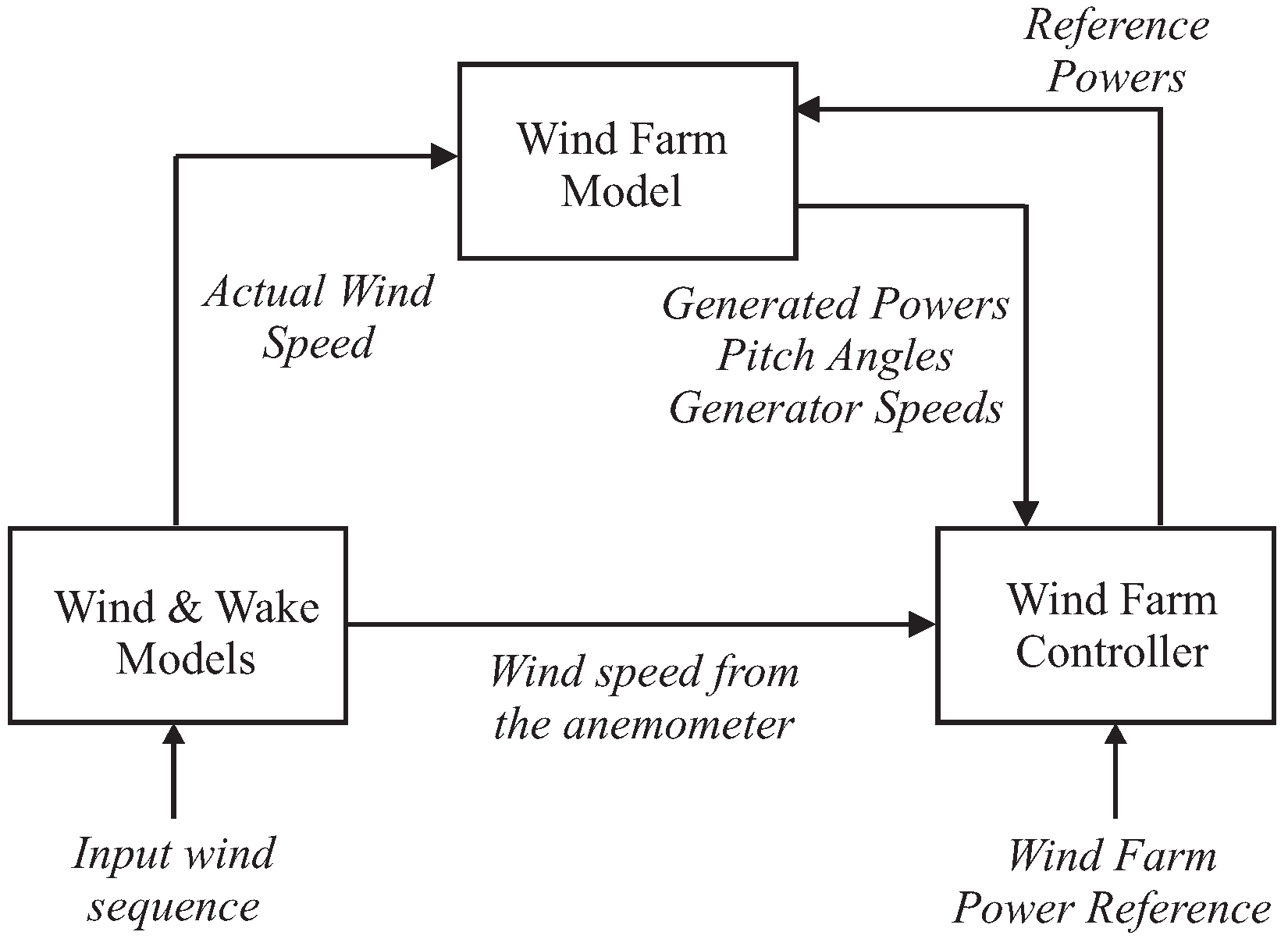
Figure 2.
The equivalent fault and measurement error description of the system under diagnosis.
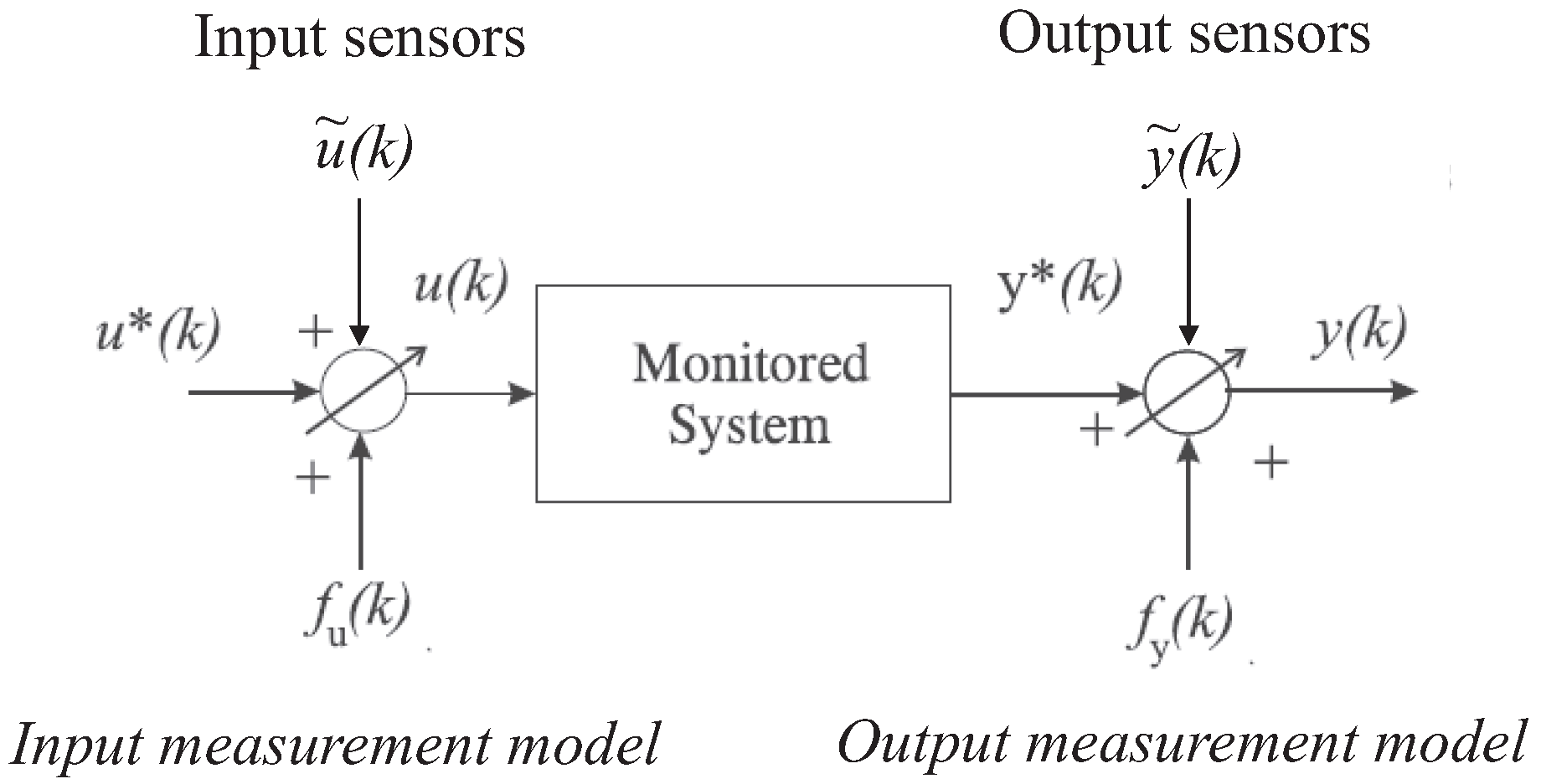
Figure 3.
The general residual generation scheme relying on fault estimators.
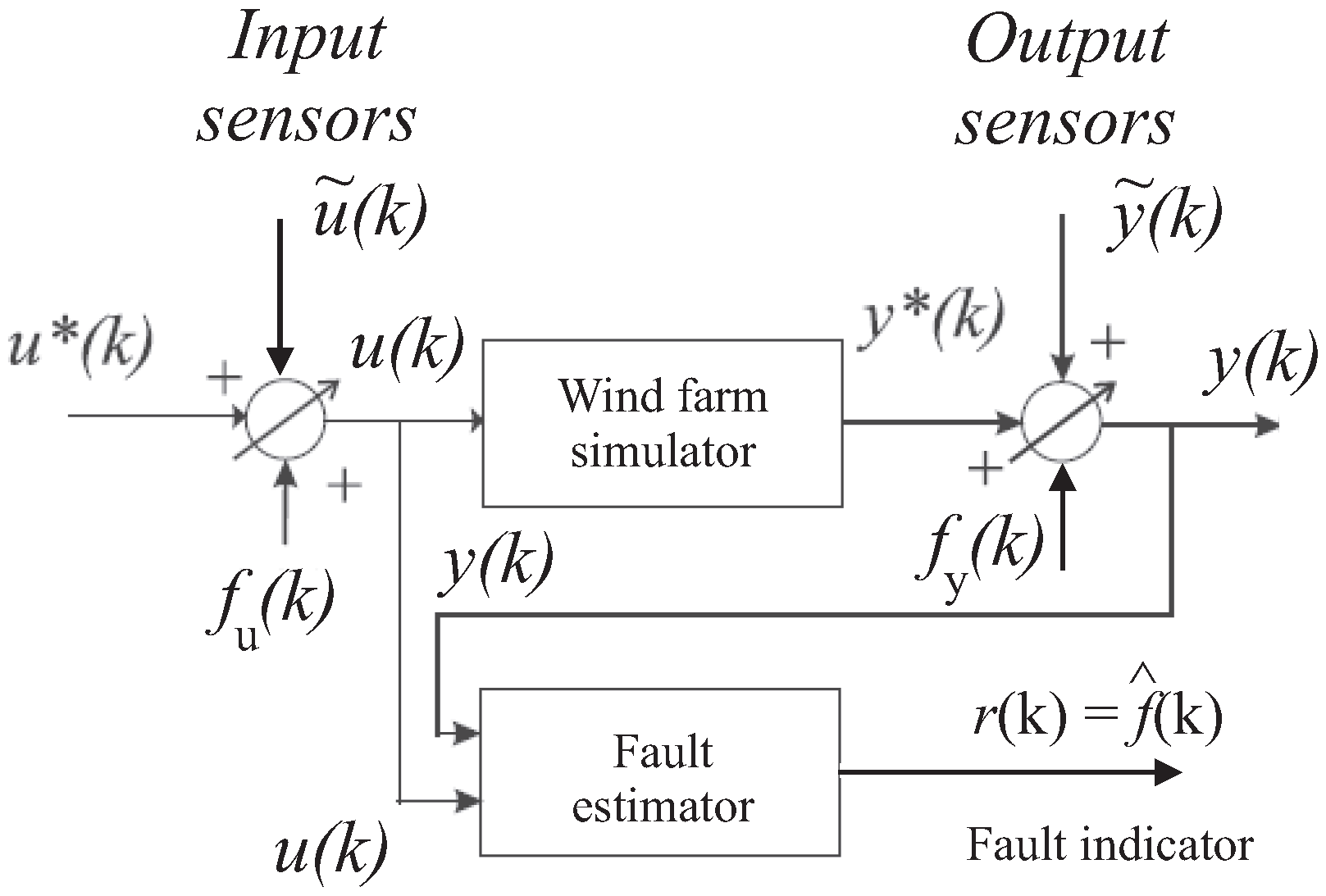
Figure 4.
The general estimator scheme for the reconstruction of the equivalent input or output faults, or .
Figure 4.
The general estimator scheme for the reconstruction of the equivalent input or output faults, or .

Figure 5.
The nonlinear autoregressive neural network with exogenus input topology (NN–NARX) used to reconstruct of the general fault signal .
Figure 5.
The nonlinear autoregressive neural network with exogenus input topology (NN–NARX) used to reconstruct of the general fault signal .
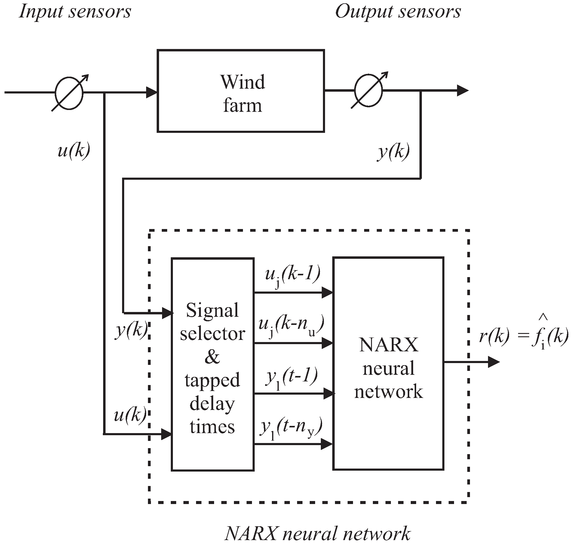
Figure 6.
Neural networks and fuzzy model similarity in the general design procedure. NN: neural network; TS: Takagi–Sugeno.
Figure 6.
Neural networks and fuzzy model similarity in the general design procedure. NN: neural network; TS: Takagi–Sugeno.
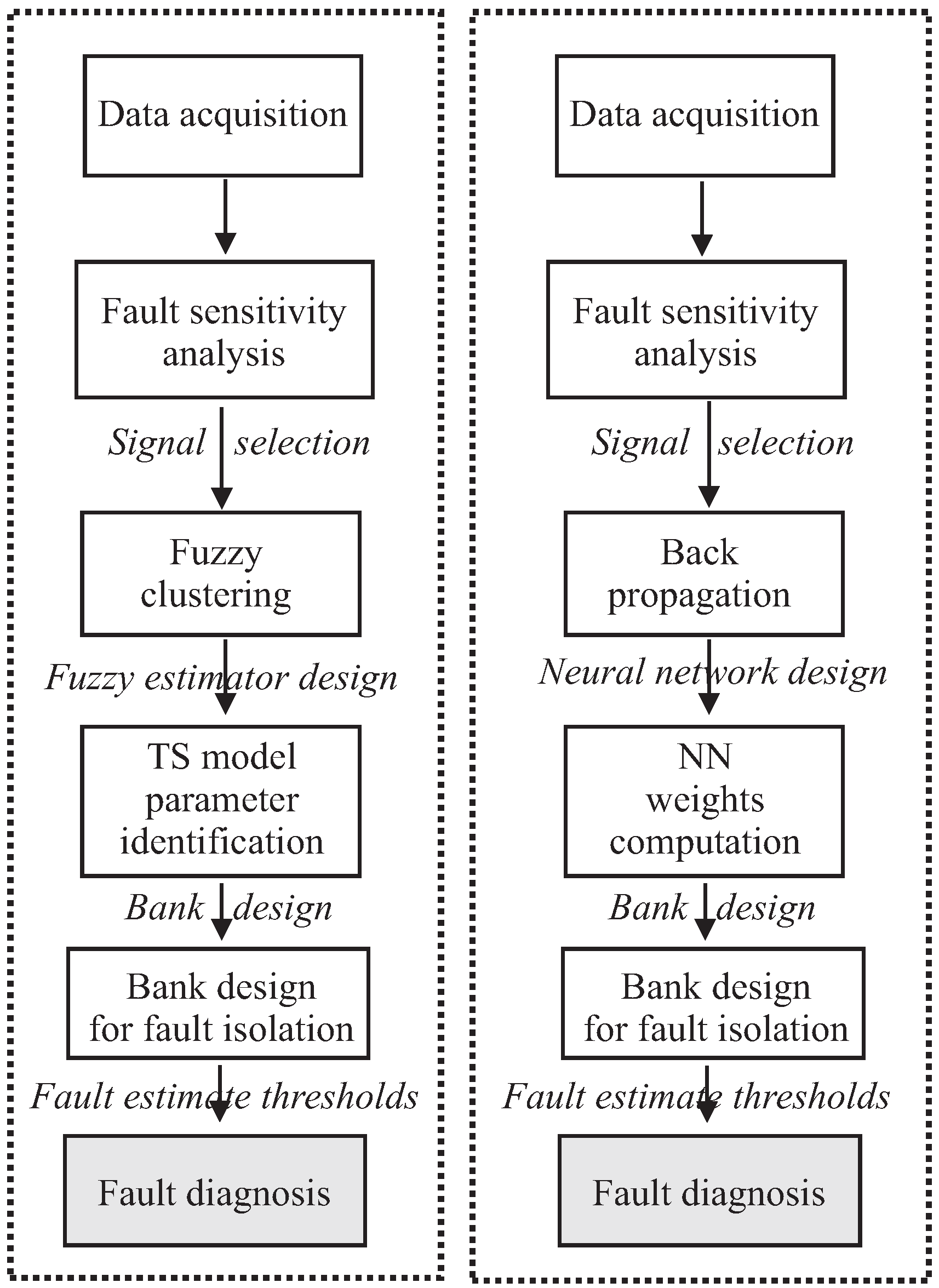
Figure 7.
The mean wind speed sequence driving the simulations of the wind farm.
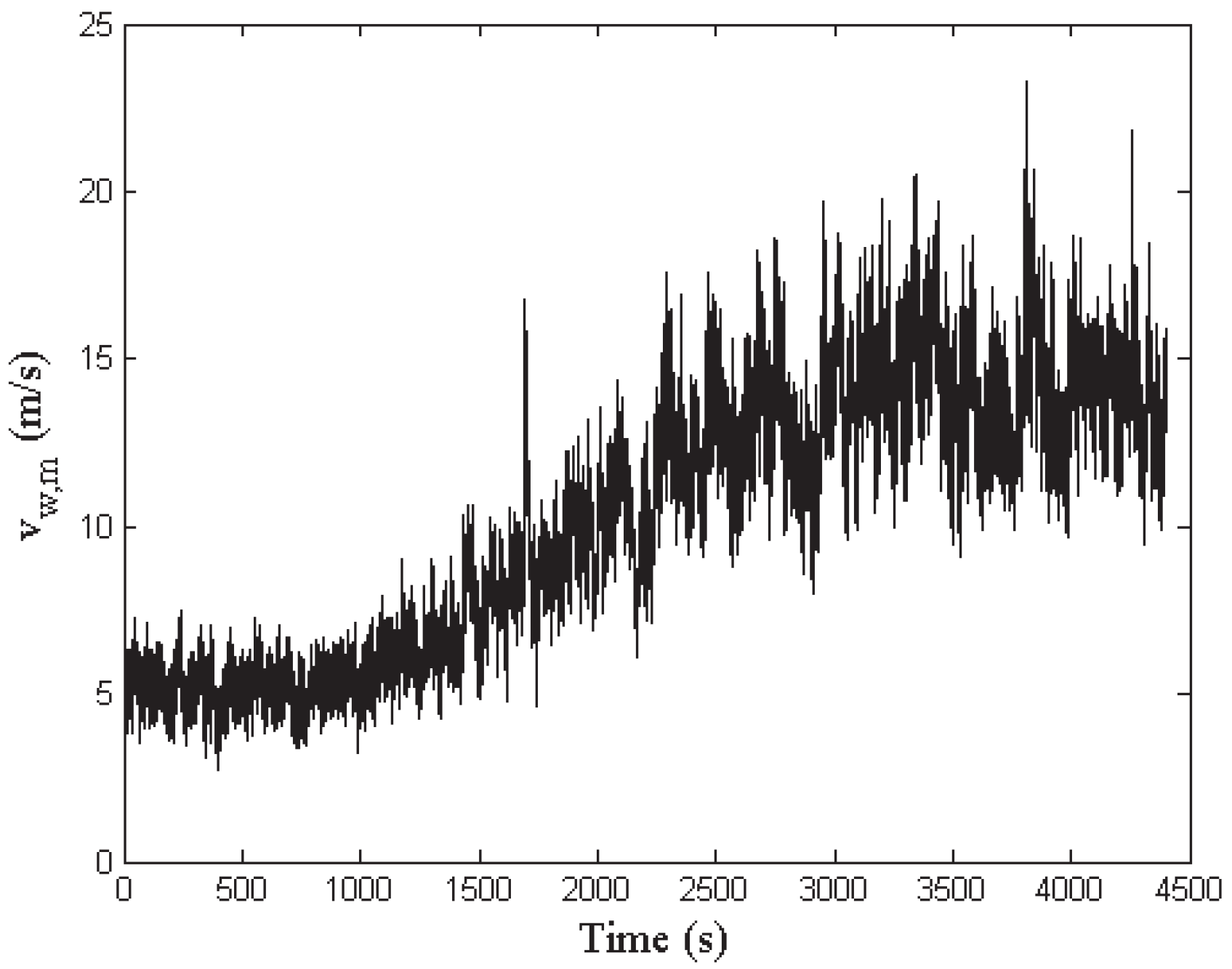
Figure 8.
Fault 1 estimator residual (continuous lines) and its threshold level (dotted line).
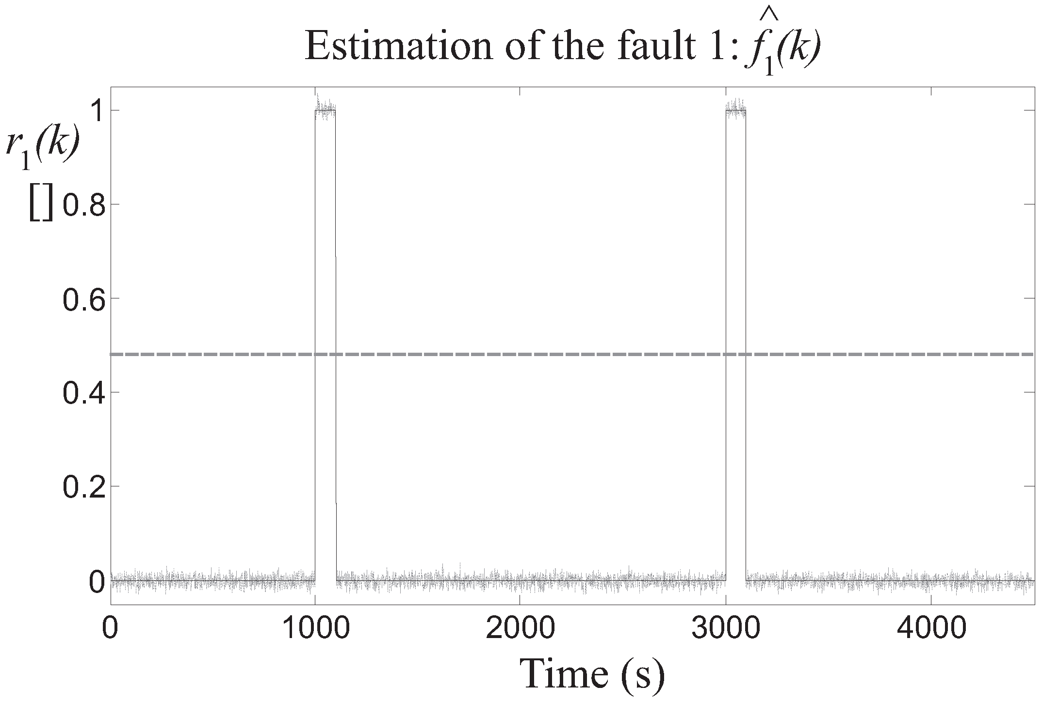
Figure 9.
Fault 2 estimator residual (continuous lines) and its threshold level (dotted line).

Figure 10.
Fault 3 estimator residual (continuous lines) and its threshold level (dotted line).

Table 1.
The fault scenarios considered for the wind farm benchmark model.
| Fault # | Fault Cause | Description | Fault Effect |
|---|---|---|---|
| 1 | Blade surface debris build-up | Scaling factor (aerodyn. model) | Reduced generated power |
| 2 | Blade misalignment | Sensor offset | Measured pitch angle offset |
| 3 | Drive-train wear and tear | Drive-train model params. | Generator speed oscillation |
Table 2.
Wind farm benchmark model parameters.
| Variable Name | Parameter Value |
|---|---|
| R | 57.5 m |
| 1.2 rad/s | |
| 1000 W | |
| 10 Hz | |
| 1.6 rad/s | |
| 158 rad/s |
Table 3.
Fault signatures for the fault estimator bank.
| Residual/Fault | … | … | ||||||
|---|---|---|---|---|---|---|---|---|
| 1 | 0 | … | 0 | 0 | 0 | … | 0 | |
| 0 | 1 | … | 0 | 0 | 0 | … | 0 | |
| ⋮ | ⋱ | … | ⋮ | |||||
| 0 | 0 | … | 1 | 0 | 0 | … | 0 | |
| 0 | 0 | … | 0 | 1 | 0 | … | 0 | |
| 0 | 0 | … | 0 | 0 | 1 | … | 0 | |
| ⋮ | … | ⋱ | ⋮ | |||||
| 0 | 0 | … | 0 | 0 | 0 | … | 1 |
Table 4.
Fault sensitivity and selected benchmark signals.
| Fault Case | Most Sensitive Measurements and |
|---|---|
| 1 | , , , , |
| 2 | , , , , |
| 3 | , , , , |
Table 5.
Faulty turbines (#, row and column indices) and fault activation times.
| Fault | # Affected Turbine: (i, j) | Time (s) |
|---|---|---|
| 1 | # 7: (3, 1) | 1000–1100 |
| # 2: (1, 2) | 3000–3100 | |
| 2 | # 1: (1, 1) | 1300–1400 |
| # 5: (2, 2) | 3300–3400 | |
| 3 | # 6: (2, 3) | 1600–1700 |
| # 8: (3, 2) | 3600–3700 |
Table 6.
Relative mean square error (RMSE) of the fuzzy fault estimators.
| 2*Data Set | RMSE (%) | ||
|---|---|---|---|
| Fault 1 Estimator | Fault 2 Estimator | Fault 3 Estimator | |
| Estimation | 0.0090 | 0.0087 | 0.0092 |
| Validation | 0.0103 | 0.0101 | 0.0105 |
| Test | 0.0108 | 0.0103 | 0.0109 |
Table 7.
Neural network performance in terms of RMSE %.
| Fault Estimator # | 1 | 2 | 3 |
|---|---|---|---|
| RMSE % (training set) | 0.0089 | 0.0091 | 0.0092 |
| RMSE % (validation set) | 0.0091 | 0.0093 | 0.0095 |
| RMSE % (test set) | 0.0106 | 0.0104 | 0.0123 |
Table 8.
The optimal values of the parameter used for fault diagnosis purposes by the designed residual generators.
Table 8.
The optimal values of the parameter used for fault diagnosis purposes by the designed residual generators.
| Residual | for the Fuzzy Estimators | for the Neural Network Estimators |
|---|---|---|
| 1 | 2.15 | 2.34 |
| 2 | 2.23 | 2.45 |
| 3 | 2.34 | 2.89 |
Table 9.
RMSE of the nonlinear differential geometric approach (NLGA) fault estimator with disturbance decoupling.
Table 9.
RMSE of the nonlinear differential geometric approach (NLGA) fault estimator with disturbance decoupling.
| Fault Case | Fault 1 Estimator | Fault 2 Estimator | Fault 3 Estimator |
|---|---|---|---|
| RMSE (%) | 0.0007 | 0.0008 | 0.0009 |
Table 10.
Monte-Carlo analysis parameter variations.
| Parameter | Nominal Value | Error Value |
|---|---|---|
| 1.225 kg/m | ||
| J | 7.794 × 10 kg/m | |
Table 11.
Comparison of the fault diagnosis results with the different fault diagnosis strategies. FF: fuzzy filter; IPE: interval parity equation; NLGA-AF: NLGA adaptive filter; NNF: neural network filter; CBD: CUSUM–based detection.
Table 11.
Comparison of the fault diagnosis results with the different fault diagnosis strategies. FF: fuzzy filter; IPE: interval parity equation; NLGA-AF: NLGA adaptive filter; NNF: neural network filter; CBD: CUSUM–based detection.
| Fault Case | Index | FF | NNF | NLGA-AF | CBD | IPE |
|---|---|---|---|---|---|---|
| 1 | FAR | 0.0010 | 0.0010 | 0.0006 | 0.0013 | 0.0024 |
| MFR | 0.0010 | 0.0010 | 0.0007 | 0.0000 | 0.0005 | |
| TFR | 0.9990 | 0.9990 | 0.9994 | 0.9999 | 0.9995 | |
| MFD (s) | 0.02 | 0.01 | 0.007 | 4.7 | 1.1 | |
| 2 | FAR | 0.0010 | 0.2280 | 0.0004 | 0.0111 | 0.0015 |
| MFR | 0.0030 | 0.0010 | 0.0005 | 0.0015 | 0.0005 | |
| TFR | 0.9970 | 0.9990 | 0.9996 | 0.9985 | 0.9995 | |
| MFD (s) | 0.08 | 0.08 | 0.008 | ND | 12.4 | |
| 3 | FAR | 0.0030 | 0.0010 | 0.0005 | 0.0055 | 0.0007 |
| MFR | 0.0080 | 0.0010 | 0.0006 | 0.0000 | 0.0010 | |
| TFR | 0.9920 | 0.9990 | 0.9995 | 0.9999 | 0.9990 | |
| MFD (s) | 0.02 | 0.01 | 0.006 | 13.1 | 15.2 |
© 2017 by the authors. Licensee MDPI, Basel, Switzerland. This article is an open access article distributed under the terms and conditions of the Creative Commons Attribution (CC BY) license (http://creativecommons.org/licenses/by/4.0/).
Share and Cite
MDPI and ACS Style
Simani, S.; Castaldi, P.; Farsoni, S. Data–Driven Fault Diagnosis of a Wind Farm Benchmark Model. Energies 2017, 10, 866. https://doi.org/10.3390/en10070866
AMA Style
Simani S, Castaldi P, Farsoni S. Data–Driven Fault Diagnosis of a Wind Farm Benchmark Model. Energies. 2017; 10(7):866. https://doi.org/10.3390/en10070866
Chicago/Turabian StyleSimani, Silvio, Paolo Castaldi, and Saverio Farsoni. 2017. "Data–Driven Fault Diagnosis of a Wind Farm Benchmark Model" Energies 10, no. 7: 866. https://doi.org/10.3390/en10070866
Note that from the first issue of 2016, this journal uses article numbers instead of page numbers. See further details here.