Small-Signal Stability Analysis of Interaction Modes in VSC MTDC Systems with Voltage Margin Control


Faculty of Electrical Engineering and Computing, University of Zagreb, Unska 3, 10000 Zagreb, Croatia
*
Author to whom correspondence should be addressed.
Energies 2017, 10(7), 873; https://doi.org/10.3390/en10070873
Submission received: 5 May 2017
/
Revised: 27 June 2017
/
Accepted: 28 June 2017
/
Published: 29 June 2017
(This article belongs to the Section F: Electrical Engineering)
Abstract
:Multi-terminal Direct Current Transmission (MTDC) is an emerging and promising technology for the transmission of electricity and the main initiator of the development of MTDC grids is offshore wind generation. However, prior to their construction, a thorough investigation of different aspects of their implementation and operation is required. In this research, an MTDC grid with voltage margin control consisting of voltage source converters (VSCs) and a high frequency cable model was implemented in Matlab/SIMULINK (R2015b, The MathWorks, Inc., Natick, MA, USA). Small-signal stability analysis was carried out to investigate the sensitivity of the grid’s interaction modes to the operating point, the structure of the grid, and the selection of the voltage controlling converter. Based on the findings of these analyses, a strategy for droop control method is proposed and demonstrated.
1. Introduction
The development of Multi-Terminal Direct Current (MTDC) grids was initiated by the vast wind power generation located far from the coastline. In such conditions, the connection of these wind-power plants via alternating current becomes technically aggravated, so direct current has become more profitable. The deployment of voltage source converters enabled the implementation of parallel DC grids and power reversal without changing voltage polarity [1]. Before the wide commissioning of these grids, researchers worldwide are investigating different aspects of their control, operation and protection [2,3,4,5,6]. In this context, small-signal stability analysis is an analytical tool that could provide answers to several questions.
Small-signal stability analysis, or modal analysis, is essential for all dynamic systems to provide detailed insight into its behavior and has been used by a number of researchers to analyze the dynamic properties of voltage source converters (VSC) within frame of high voltage direct current transmission (HVDC). Many studies have used modal analysis and participation factor analysis to investigate the interactions between the MTDC grid and AC grid [7,8]. It was shown that there a clear distinction existed between the modes corresponding to AC and DC grid states. In [8], a sensitivity analysis of the control modes was performed with respect to gains in voltage droop control and converter capacitance. Similar research was done in [9] where investigators also explored the sensitivity of eigenvalues to droop gains and the capacitance of the DC link. A detailed impact of VSC controls on the stability of MTDC grid and connecting AC system was completed in [10,11]. Small-signal analysis was used to show that maximum power transfer capability of a VSC-HVDC converter was dependent on gains of the Phase Locked Loop (PLL) and the Short Circuit Ratio (SCR) of the system. Furthermore, a few studies have been undertaken to explore the sensitivity of eigenvalues of the MTDC grid with respect to the operating point of the system. In [12] the authors tracked the eigenvalues of two-terminal and three-terminal systems under different loading conditions, i.e., operating points and different gains of the direct-voltage controller. However, they did not undertake a thorough analysis of certain modes.
Like the AC system, oscillations modes can be divided into local and interarea modes. The importance of interarea modes lies in the interaction of two converters which deteriorates the desired control actions. In [13], researchers established a methodology for identifying the interaction modes and conducted a parametric sensitivity analysis of the interaction modes with respect to line inductance (simulating effects of DC circuit breakers) and variations of droop gains within voltage droop control.
Multi-terminal DC grids, in this article, were modelled with margin control for two reasons. First, the number of interaction modes with such control is smaller than droop control—as shown in [13]—which makes analysis simpler. Second (and more importantly), this method has some basic concepts for system control that have been determined that could possibly be generalized to droop control. As the sensitivity of interaction modes in a DC grid with respect to the operating point and structure of the grid have not been investigated thoroughly thus far, it was the main objective of this work. Furthermore, this study also examined the analysis of the dominant interaction mode with respect to the selection of a voltage controlling converter. A voltage controlling converter is mostly selected upon circumstances in connecting an AC grid; however, by using this method, another selection criteria is established.
Modeling the DC grid consisting of VSC converters and cables is described in Section 2. Small-signal stability analysis and the methodology for identifying interaction modes from [13] are described in Section 3 and applied on a simple three-terminal DC grid. Section 4 and Section 5 present the results and discussion of the proposed analyses. A synthesis of the obtained conclusions and prospects for future work are given in Section 6.
2. Modeling of Multi-Terminal Direct Current Grid
2.1. Dynamic Model of Voltage Source Converter
The lossless time-averaged dynamic model of the two-level pulse width modulation (PWM) VSC converter was taken and adjusted from References [14,15]. Detailed electromagnetic modeling of electronic devices is not necessary for the purposes of electromechanical studies. The model consists of two main parts: the physical model, and control scheme (Figure 1, adopted from Reference [15]). The physical model has three main parts: the AC system (transformer and phase reactance), DC system (converter capacitance), and the converter which connects the AC and DC side using the law of power conservation. Because of using averaged switched converter model—the higher harmonics of switching are neglected and capacitor filter on the AC side is omitted. Vector control is a standard method for controlling the VSC converter because of the possibility to independently control active and reactive power. For this reason, it is necessary to transform electrical quantities into a dq-reference frame and align one of the axis with the voltage on the Point of Common Coupling (PCC) using referent angle , which is determined by the Phase Locked Loop. Character marks voltage on the point of common coupling and converter AC voltage. Direct current is denoted by and direct voltage by .
Dynamics of the AC currents in dq-reference frame () of Converter are described with the following equations:
where is transformer reactance; and are the reactance and resistance of phase reactor; and is angular frequency. Dynamics of the DC side is described with:
where stands for the equivalent DC capacitance (which includes capacitance of converter and belonging cables); and is the DC current between the converters (nodes) and . The positive sign marks the current entering the node and the negative sign is the current leaving the node. Law of conservation of power couples AC and DC sides:
Converter losses are neglected. Coefficient 2 in Equation (3) marks the bipolar operation of the converter. In the case of a monopolar operation, this coefficient would be equal to one. The control scheme has a hierarchical structure composed of outer control loops and inner control loops, which can also be seen in Figure 1. Every control loop consists of a standard PI regulator of transfer function:
The output of every regulator is limited, which is also one of the advantages of vector control, but for simplicity reasons limiters are not shown in Figure 1 and are not used in converter modeling. Furthermore, the control scheme differs whether the converter is in rectifier or in inverter operation mode. For rectifier operation, inputs to the outer control loops are the referent active power and the referent reactive power (or AC voltage ), while for the inverter operation inner control loop for DC voltage is omitted and DC voltage is set to (marked with green in Figure 1). An outer control loop for reactive power (or AC voltage) is also present in inverter operation mode. Outputs of the outer control loops are referent dq-current values and , which are inputs to the inner control loops. Outputs of this control level are referent converter AC voltages and , which are transformed back to the abc-quantities and are used for calculation of modulation indices. Inverter q-component of current is calculated using an output of DC voltage outer loop and equation (3). More details upon modeling of VSC control can be found in [14].
Thus, the state vector of the rectifier consists of nine variables and state vector of inverter consists of eight variables . State variables and are connected with the inner current control , and are state variables connected with the outer and DC voltage control; and and are state variables connected with PLL.
2.2. Frequency Dependent Cable Model
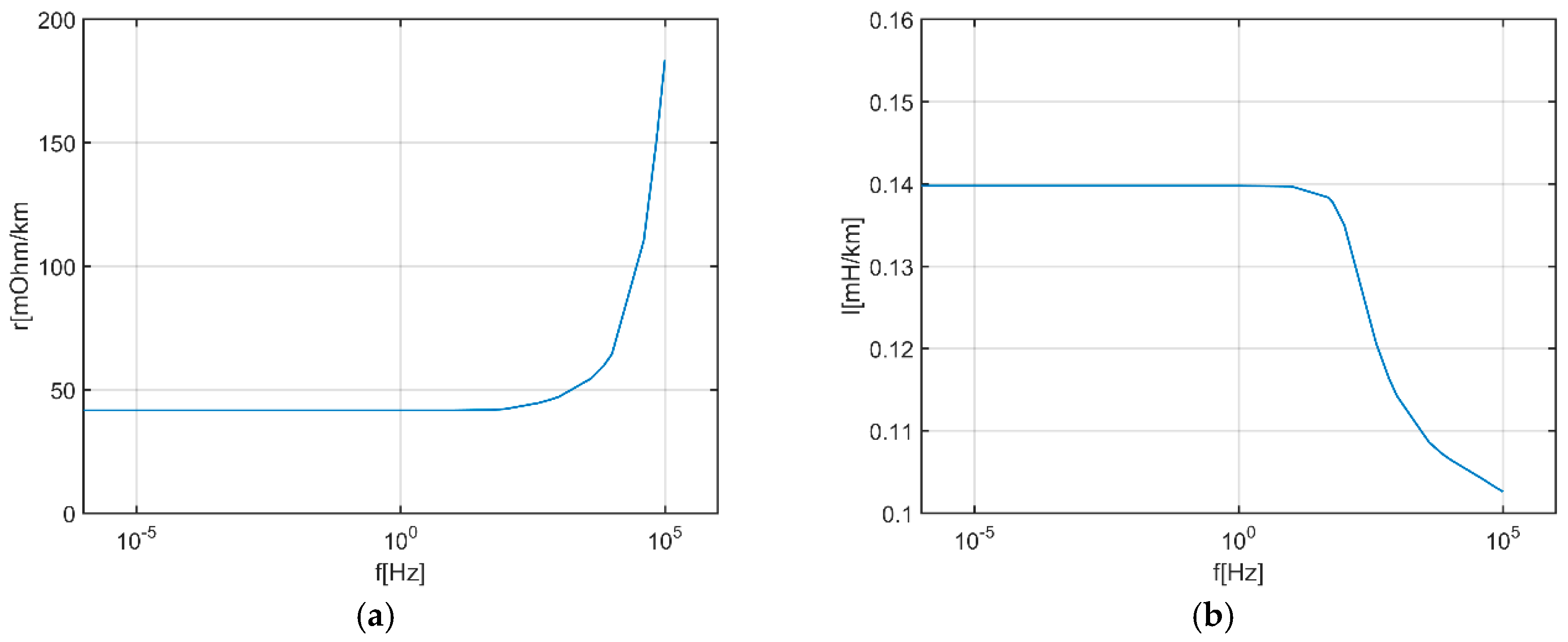
A vector fitting method was used for modeling frequency dependent cable parameters ([16,17,18]). The model consisted of several π sections that accounts for distributed line parameters (correction factors), while in each π section there is a connection of multiple series branches. Cable model without frequency dependency can lead to false conclusions on the stability of HVDC systems. More details can be found in [19], and based on the experience of this article, the cable model with five parallel sections each with three series branches was used (Figure 2). The state-space representation of this cable model had 21 states (15 branch currents and six voltages). The typical frequency dependency of cable resistance and inductance can be found in the Appendix A. Here, it is important to emphasize that there also exist other methods for modeling frequency dependent cable parameters, but our approach—taken from [19]—is adjusted for state-space representation.
3. Small-Signal Stability Analysis and Identification of Interaction Modes
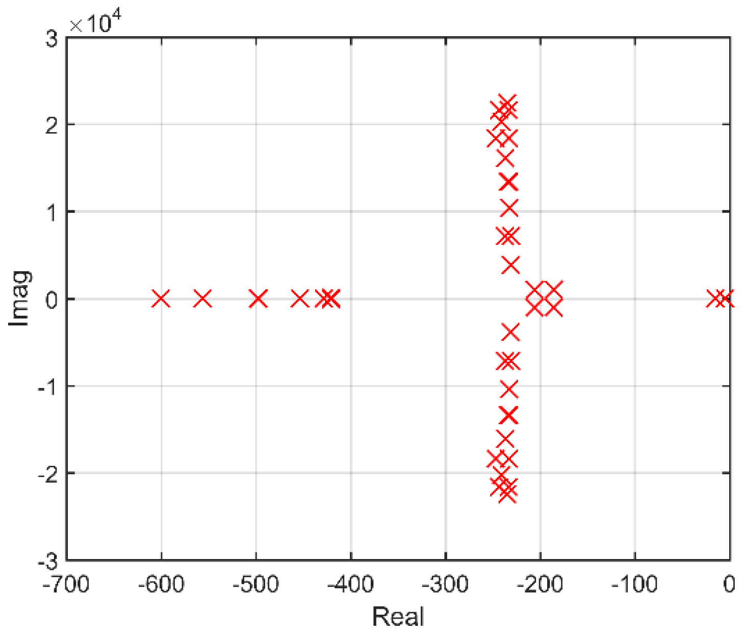
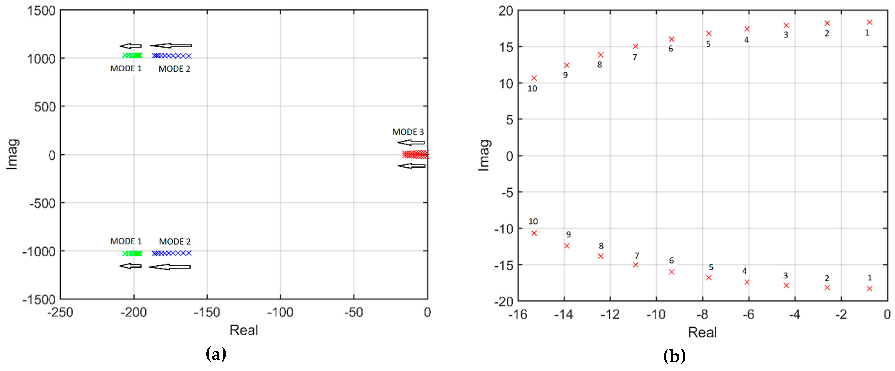
A radial DC grid consisting of three converters and four nodes (Figure 3) was built in Matlab/SIMULINK (R 2015b, The MathWorks, Inc., Natick, MA, USA). The electric and control parameters of all converters were equal and are given in the Appendix A, where the electric parameters of the cables are also provided. The powers of converters were equal to (inverter), and (rectifiers), and all line lengths were equal to 100 km. One converter (Converter 1) regulated DC voltage to referent voltage (1 pu), while other converters regulated real power, i.e., voltage margin control employed in the grid. The model was linearized around the operating point using the Matlab linearizing tool and the system eigenvalues and eigenvectors were obtained. There were 84 states in the systems and therefore 84 eigenvalues. Figure 4 shows the eigenvalues with their real parts limited to −1000.
Certain eigenvalues are more stable if its real part is more negative, i.e., further from the origin of the coordinate system. The inverse value of the absolute real part of eigenvalue corresponds to the time constant of amplitude decay of that eigenvalue. For oscillatory mode there is also a defined value called the damping ratio [20]:
Both the inverse value of absolute part and damping ratio are used mutually to express the damping degree of the oscillatory modes.
Modes are classified as local modes if they are connected to states from only one subsystem, or interaction modes if they are connected to states from several subsystems. To determine whether a particular mode is local or interaction, a participation factor analysis was conducted. The participation factor of state variable in eigenvalue is defined in the following way [20]:
It is a product of the kth element of the ith right eigenvector or observability vector () and the ith left eigenvector or controllability vector (). Participation factor is a measure of sensitivity of the ith eigenvalue to kth state variable . Vector contains participation factors connected with the ith eigenvalue and all system states. If we divide certain participation factors with where denotes L1-norm, the normalized participation factor is obtained.
State variables of the system can be divided in groups depending on which subsystem they belong. Vector contains participation factors of mode i and state variables of subsystem . In the grid in Figure 3, three subsystems were considered: Converter 1, Converter 2, and Converter 3. Coefficient is defined in the following way [13]:
This coefficient is a measure of correlation of the ith mode to the state variables of subsystem . The mode is classified as an interaction mode if there exist at least two coefficients for which they are higher than some threshold, i.e., . In this research threshold was chosen sufficiently small (5%) to involve dominant mode relevant to small-signal stability analysis. By setting the threshold thus low, some other, less significant modes are also included in this classification as interaction modes.
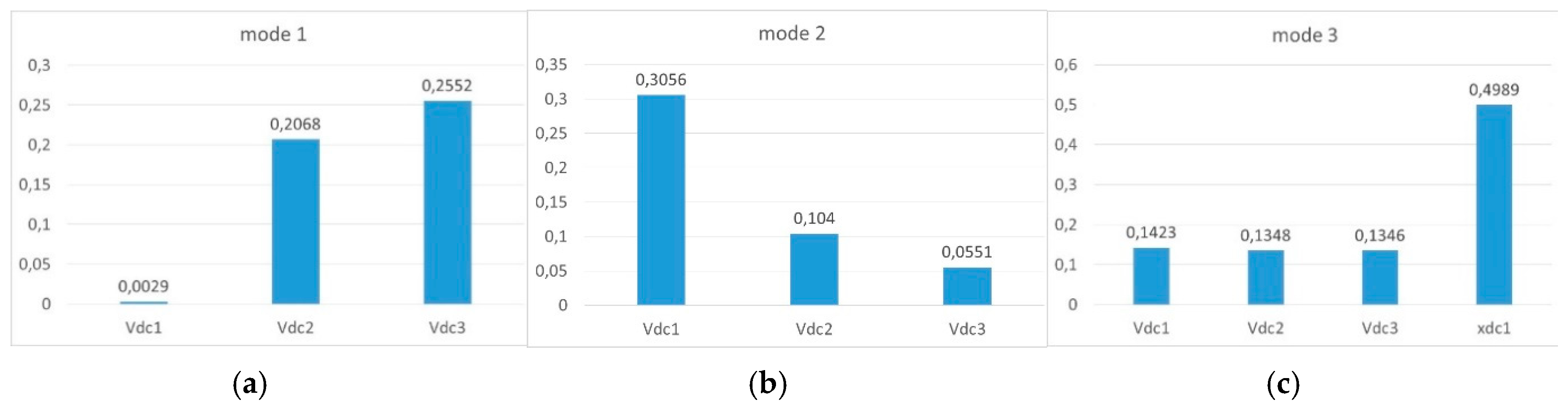
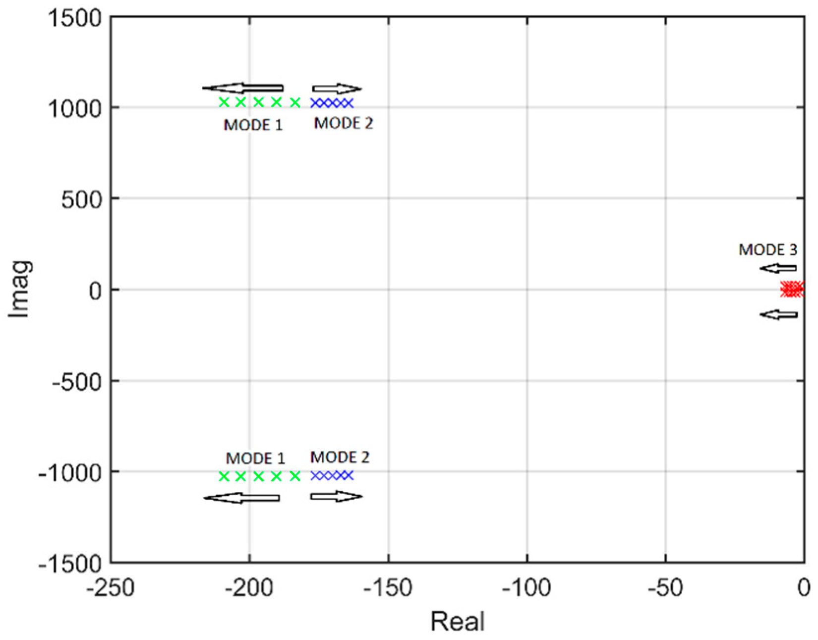
After a described analysis was conducted, there were three interaction modes in the grid from Figure 3, and are shown in Figure 5 where , and . Figure 6a–c exhibit normalized participation factors of these three modes and the state variables of the converters. There were only four state variables present: , , and , while the participation factors of other state variables were negligible in these interaction modes. Modes 1 and 2 depend on the state variables of converter voltages and Mode 3, along with voltages, mostly depends on the state variable of the direct voltage regulator. Of these three modes, the most significant one is Mode 3 as its real part is the closest to the origin of a complex plane, which results in the visibility of this mode in system response called the dominant mode.
4. Sensitivity of Interaction Modes to Operating Point and Structure of the Grid
This section contains the results and discussion of the sensitivity analysis of interaction modes in the grid to the operating point and to some extent, to the structure of the grid. All simulations were conducted using the grid in Figure 3. In Section 4.1, powers of all converters in the grid varied linearly and equally. Section 4.2 observed the grid's small-signal stability when the power of the power controlling converter was held constant, while in Section 4.3, the power of the voltage controlling converter was held constant. Section 4.4 investigates the influence of the line lengths and Section 4.5. deals with the magnitude of the referent voltage. In all study cases, Converter 1 was always in charge of the voltage control in the grid while Converters 2 and 3 regulated active power. Lengths of all lines were equal to 100 km, except in Section 4.4. where different line lengths were emphasized.
4.1. Varying Powers of All Converters
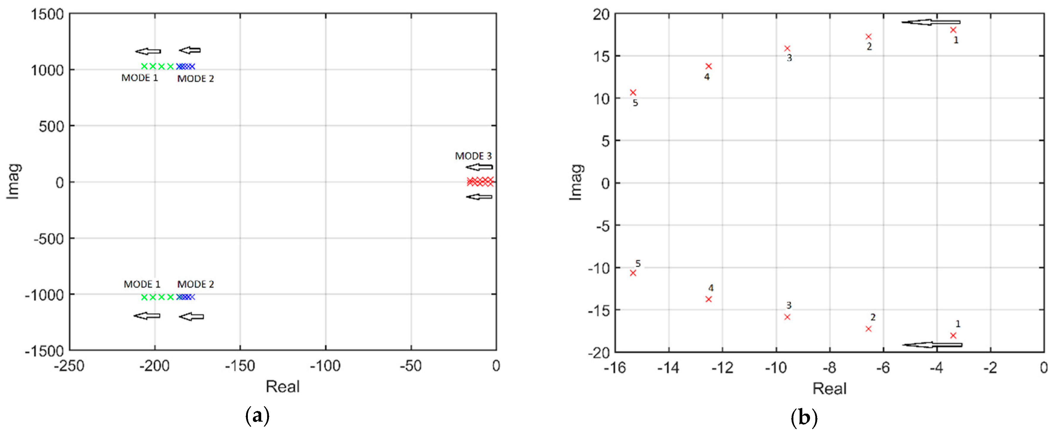
The operating state of the grid varies as per Table 1. Powers of all converters increased linearly and equally. Converter 1 operated in inverter operation mode, while Converters 2 and 3 operated as rectifiers. Table 1 contains the interaction modes and their damping factors, which are graphically depicted in Figure 7a,b.
The real parts of all three interaction modes moved to the left in the complex plane designated by the arrows in Figure 7 and damping factors of all modes increased. The grid became more stable with increased transmitted power. Change was most prominent in the most significant (dominant) interaction Mode 3. This can be explained by the fact (as we have seen in the previous section on participation factors in Figure 6a–c that Modes 1 and 2 are mostly dependent on direct voltage state variables, while Mode 3 (apart from direct voltages) is also depended on the state variable of direct voltage controller (). Here, it is important to emphasize that the described behavior of Mode 3 is valid in the range in which this mode has oscillatory shape. This also applies for other considerations in the rest of the article regarding this mode.
Small-signal analysis was verified through time-domain simulations shown in Figure 8a,b. In the 10th second referent voltage of Converter 1 changed from 1 to 1.02 pu. With the smallest powers in the grid (Point 1) voltage transitions had the highest amplitude of oscillations and were the least damped. By increasing the converter powers, voltage response became less oscillatory and more damped. The oscillatory frequency of dominant modes in Table 1 could also be noticed in Figure 8 for lower converter powers.
In cases where there are two inverters and one rectifier in the grid, the behavior of interaction modes becomes slightly different. The powers of converters and interaction modes with their damping factors are listed in Table 2 and the interaction modes are shown in Figure 9. We noted that Mode 2 became less stable as it moved to the right side of the complex plane and its damping factor decreased. Of importance was that dominant Mode 3 behaved in the same way as in the previous example.
4.2. Power of Power Controlling Converter is Held Constant
In this case, the power of Converter 2 (power controlling converter) was held constant, while the powers of Converters 2 and 3 varied. Operating points with interactions modes and their damping factors are shown in Table 3. All interaction modes in this scenario became more stable, as can be seen in Figure 10. A strong correlation between the stability of Mode 3 and power through Converter 1 (voltage controlling converter) was observed.
4.3. Power of Voltage Controlling Converter is Held Constant
This scenario differed in the fact that the power of voltage controlling converter was now held constant (Converter 1) while the powers of the other two converters varied (Table 4). Figure 11 shows the damping factors of all three interaction modes. Modes 2 and 3 were the most stable in the middle of the characteristics and Mode 1 was the least stable in this area (this was also true for the real parts of interaction modes). The operating point in the middle of the characteristics (point 8) corresponded to the most symmetrical state in the grid, with the most similar powers of Converters 2 and 3.
Here, it was also interesting to look at the participation factors of all interaction modes and how they changed with different operating points (Figure 12a–c). It arose that Mode 1 mostly depended on the voltage state(s) of corresponding rectifier(s). First, at several points, only Converter 2 injected power into the DC grid, then both Converter 2 and Converter 3 injected power, and at the last several points only Converter 3 injected power in the DC grid. A similar observation was valid for Mode 2 which mostly depended on the voltage state(s) of the corresponding inverter(s). The participation factors of Mode 3 stayed unchanged through all operating points in Table 4. Thus, it was concluded that from the participation factors of Mode 1 or Mode 2, we could approximately conclude if the converter was in rectifier or inverter operation mode.
4.4. Varying Electrical Distance between Converters
The line lengths to all three converters increased linearly and equally and the results are shown in Table 5 and in Figure 13a,b. The powers of the rectifiers remained the same while the power of the voltage controlling inverter slightly changed due to the different losses in the system. All interaction modes moved to the right of the complex plane, which means decreased stability. On the other side, the damping factors of Modes 1 and 2 increased due to a larger amount of resistance in the grid, but the damping factor of Mode 3 nevertheless decreased. Additionally, all modes behaved in the same way in the case of two inverters and one rectifier in the grid.
4.5. Varying Referent Voltage
The goal of this section was to examine how the magnitude of referent voltage affected the stability of the interaction modes. It was observed in Table 6 and Figure 14a,b that the stability of all modes decreased with higher voltages as both time constants of amplitude decay were increased and the damping factors were decreased in this case. The change was expressed the most in Mode 3, and the least in Mode 2. When there were two inverters and one rectifier in the grid, Modes 1 and 3 became less stable and Mode 2 more stable with increased referent voltage (and also with the slightest change).
5. Analysis of Dominant Interaction Mode to Selection of Voltage Controlling Converter
The goal of this study was to determine what the best location was, i.e., which inverter was the most appropriate to control the voltage in the grid, with respect to the stability of the interaction modes. In this section, only the mode with the lowest absolute value of real part was observed for two reasons: this mode mostly affects the response of the system and this mode (as seen from the participation factor analysis) is mostly affected by the state variable of the voltage regulator at the voltage controlling converter. Tests in Section 5.1, Section 5.2 and Section 5.3 were carried out on the same grid as Figure 3 where one converter operated in rectifier mode (Converter 1) while the other two converters operated in inverter mode (Converters 2 and 3). For simplicity reasons, the cable model with one PI section and one series branch was used. Rectifier voltage () was always held at 1 pu.
5.1. Two Inverters with Different Powers and Equal Line Lengths
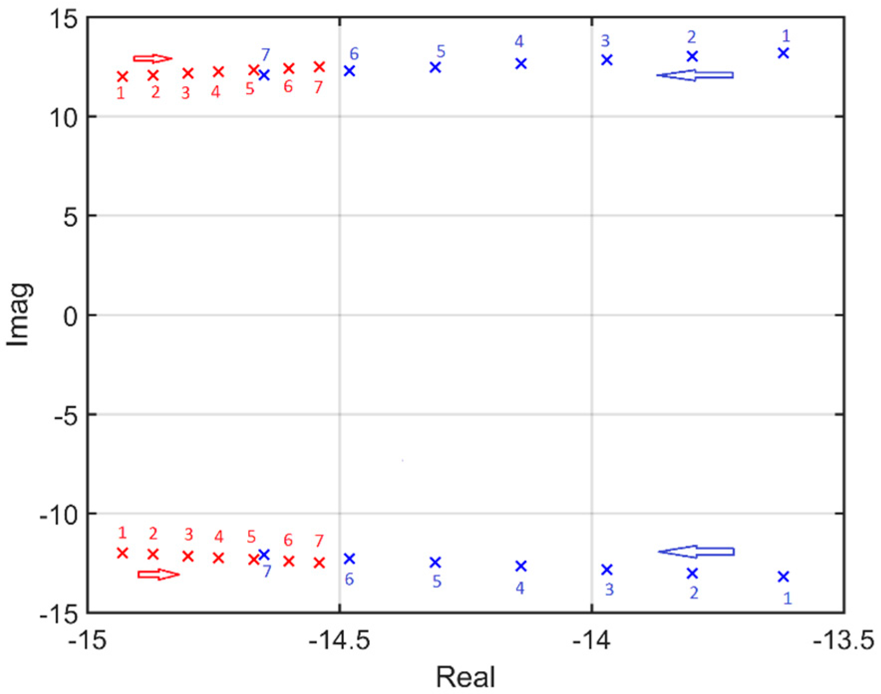
All line lengths were equal to 100 km. The power of Converter 3 changed in steps of 1 MW as seen in Table 7, together with the converter voltages and currents and dominant interaction modes in two cases: when Converter 2 controlled voltage in the grid and when Converter 3 controlled voltage in the grid. These modes are depicted in Figure 15: red for Converter 2 and blue for Converter 3. While increasing the power of Converter 3, the dominant interaction mode when Converter 3 was in charge of voltage control became more stable (as we have seen previously due to greater power) and the dominant interaction mode when Converter 2 was in charge of voltage control became less stable in this situation, which is indicated by the arrows in Figure 15. This was valid for both the real parts of the interaction modes and the damping factors of the interaction modes. A greater stability of dominant interaction mode in this case was achieved when the voltage controlling converter was the one with the greater power (or current). Of course, when the powers (currents) of the converters were equal, the corresponding modes were also equal.
5.2. Two Inverters with Equal Powers and Different Line Lengths
The powers of Converters 2 and 3 in this case were to be held equal to 100 MW, but the length of the line to Converter 3 was changed from 90 to 110 km in steps of 5 km. The length of the line to Converters 2 and 3 were constant to 100 km. Table 8 contains all important data (line lengths to Converter 3, converter powers, voltages and currents, interaction modes in two cases), and dominant interaction modes are also depicted in Figure 16. The interaction mode when Converter 2 was in charge of voltage control became less stable, and the stability of the interaction mode when Converter 3 was in charge of voltage control slightly changed (the magnitude of the amplitude decay became lower, but the damping factor became higher). From Table 8, it can be seen that the mode was more stable if the corresponding converter had a smaller voltage and consequently higher current (as powers of both converters were equal). Thus, we concluded that converter current can provide better insight into the small-signal stability of the grid.
5.3. Two Inverters with Different Powers and Different Line Lengths
In this study, the case power of Converter 3 again changed in steps of 1 MW, but differently from Section 5.1. The line lengths to Converters 2 and 3 were different: 100 km to Converter 2 and 60 km to Converter 3 (line length to Converter 1 was equal to 100 km). From Table 9 and Figure 17, it was seen that the interaction mode became less stable when the voltage controlling converter was Converter 2 (red) and the interaction mode became more stable when the voltage controlling converter was Converter 3 (blue) by increasing the power of Converter 3. The real parts of the interaction modes were equal when the power of Converter 3 was 105.5 MW and their damping factors were equal when the power of Converter 3 was slightly below 105 MW. Currents of these two converters were equal with a power at Converter 3 of 101.6 MW. In future avenues of this work, we will consider only real parts of interaction modes as a measure of their stability. This will not affect the results and conclusions as these two parameters of interaction mode (real parts and damping factors) behave in the same way and the corresponding converter power does not much differ.
The same procedure was repeated with different line lengths to Converter 3 and the results are depicted in Figure 18. The powers of Converter 3 are in the middle of the figure (x-axis) and the line lengths are on the left side of the figure (y-axis). Blue lines mark the power of Converter 3 when it had the same current as Converter 2, and red lines mark the power of Converter 3 when they had the same real parts of dominant interaction modes (with respect to Converter 2 with a power of 100 MW and line length of 100 km). Left from the blue lines was an area of lower current, and right from the blue lines was an area of higher current (compared with the Converter 2 current). Likewise, left from the red lines was an area of lower stability, and right from the red lines was an area of higher stability of the dominant interaction mode (in comparison to the dominant interaction mode when Converter 2 oversaw voltage control). The following conclusion was drawn: if a converter of a greater power has a lower current, then the stability of the dominant interaction mode is lower (when it is in charge of voltage control) and if a converter of smaller power has a higher current, then the stability of the dominant interaction mode is higher (when it is in charge of voltage control). However, the opposite does not work, i.e., if a converter with a greater power has higher current, we do not know if the stability of the dominant interaction mode is higher or lower (when it is in charge of voltage control), or if a converter of lower power has a lower current, we do not know if the stability of the dominant interaction mode is higher or lower (when it is in charge of voltage control). These conclusions help us to make assessments on the stability of the dominant interaction mode without carrying out a small-signal stability calculation of the grid. Similar conclusions can be drawn using converter voltages instead of currents, so in the continuation of this study, the formulation using converter currents will be used.
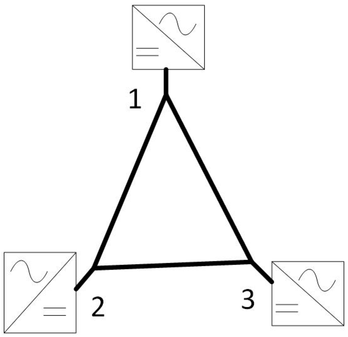
5.4. Triangular DC Grid
The tests conducted in Section 5.1, Section 5.2 and Section 5.3 were repeated on a simple triangular grid shown in Figure 19. The goal was to determine whether the structure of the grid—delta or star connection of converter cables—affected the derived conclusions. For these reasons, the star-delta transformations of cable resistances (cable lengths, respectively) were conducted by well-known expressions:
Thus, the voltage and currents of all converters remained unaltered. Such grids have three interaction modes and their values do not differ much from the case of a star connected grid. Again, only the mode with the lowest absolute value of the real part was observed. In all cases, as in previous sections, Converter 1 worked in rectifier operation mode while Converters 2 and 3 worked in inverter operation mode. In the first case, all line lengths equaled 300 km, calculated by Equation (7), and the results of varying Converter 3 power are shown in Table 10. When the voltage controlling converter was the one with greater power, the dominant interaction mode had greater stability.
In the second case, the line lengths were varied based on data from Table 11 and the power of Converters 2 and 3 were equal to 100 MW. It was seen that the dominant interaction mode was more stable when the corresponding converter had a greater current (and consequently lower voltage). In the third case, the line lengths were equal to: , and ; the power of Converter 2 was held constant at 100 MW; and the power of Converter 3 varied (Table 12). The same real part of the dominant interaction mode was achieved when the power of Converter 3 was slightly above 105.5 MW and the same damping factor when the power of Converter 3 was slightly below 105 MW, in comparison to the scenario when Converter 2 oversaw voltage control in the grid. These results are slightly different to the values obtained in Section 5.3. Converter 3 had the same current as Converter 2 at a power of 101.6 MW. In the same way as Section 5.3, it was concluded that if a certain converter of greater power had a lower current, then the stability of the dominant interaction mode (when this converter oversaw voltage control in the grid) was certainly lower compared to the scenario when another converter was in charge of voltage control.
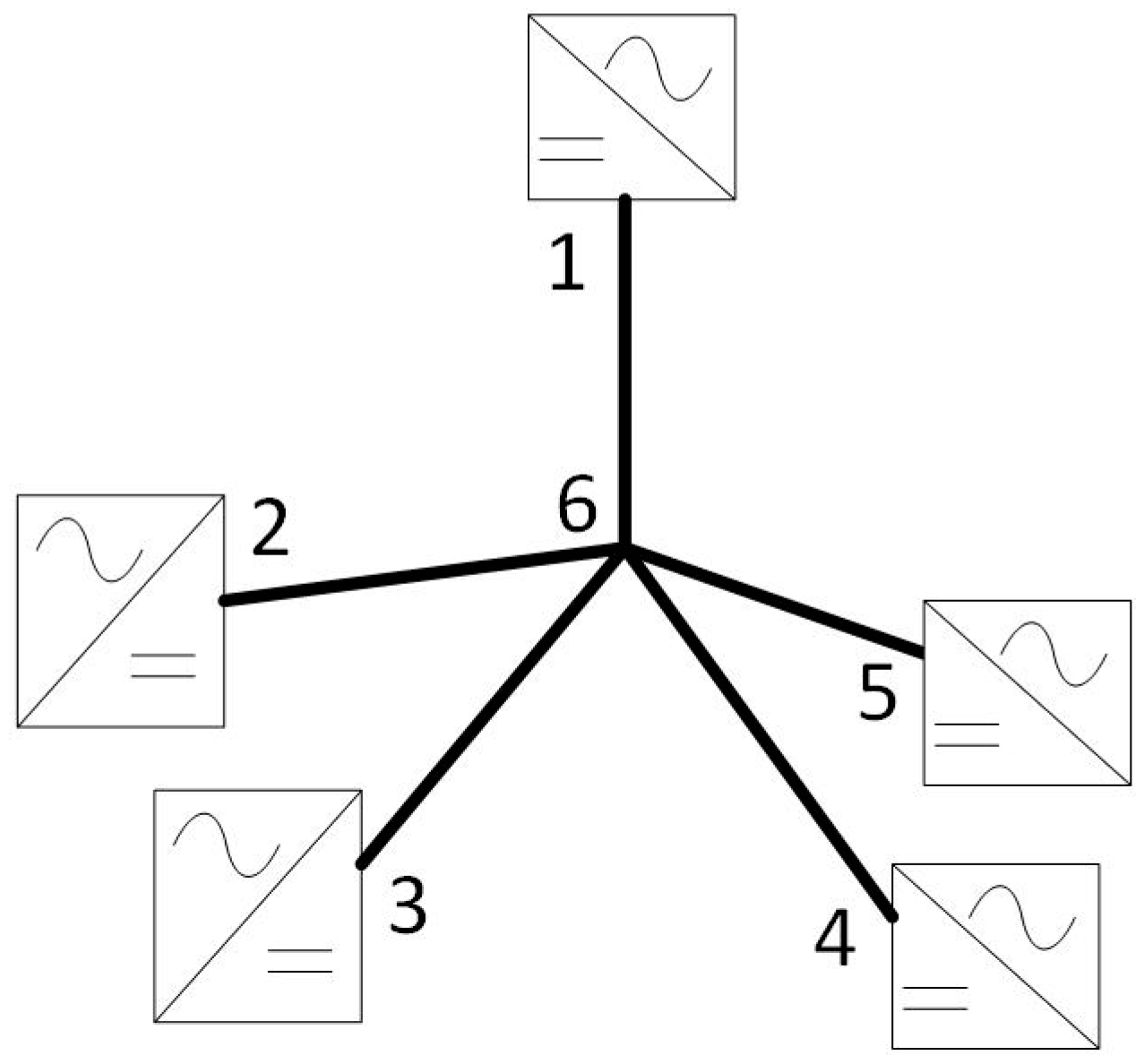
5.5. Radial DC Grid with Multiple Nodes
Derived conclusions were examined on a radial five node grid (Figure 20) to generalize these conclusions to any radial or star-connected grid. Converter 1, as in previous sections, was in rectifier operation mode, and other four converters were in inverter operation mode. In the first case (Table 13), corresponding line lengths for all inverters were equal, but their powers differed. The most appropriate converter for grid voltage control with respect to the stability of the dominant interaction mode was, as expected, the one with the greatest power (Table 13).
In the second case, all inverters had the same powers, but their line lengths from the central node were different. The converter with the most stable dominant interaction mode was the one with the longest corresponding line length, i.e., the one with the highest DC current (and the lowest DC voltage). The relevant data is given in Table 14.
In the third case, line lengths of all inverters were different again, and their powers were equal except for the power at Converter 2, which was slightly higher (Table 15). Although the power of Converter 2 was higher than the power at Converter 5, the current at Converter 2 was lower than the current at Converter 5. For this reason, the dominant interaction mode when Converter 2 was in charge of voltage control was less stable than the scenario when Converter 5 was in charge of voltage control in the grid. The current of Converter 2 was higher than the currents at Converters 3 and 4, so general conclusions on the stability of corresponding interaction modes without conducting a small-signal stability calculation could not be made.
These conclusions cannot be generalized to grids in general polygon configurations.
However, these considerations in a grid with voltage margin control could be helpful for the determination of droop coefficients in the droop control method to ensure the highest possible small-signal stability. If the sequence of converters, with respect to the stability of the dominant interaction mode, is known (in voltage margin control) then the droop gain magnitudes should follow that sequence to ensure the highest stability of the dominant interaction mode. Droop control is described with the following equation:
where is a coefficient of droop control; and and are the referent active power and direct voltage of a certain converter. This control loop is added on the active power outer control loop. When voltage in the grid rises, the inverters need to increase their active power and the rectifiers need to decrease their active power. So, as defined in Equation (8), inverters have positive droop gains and rectifiers have negative droop gains. Converters with higher absolute values of droop gains participate more, and the ones with lower absolute values of droop gains participate less in voltage control of the grid. Margin control can be considered as a marginal case of voltage droop control where one converter has an infinite droop gain (voltage controlling converter) and others have zero droop gains (power controlling converters). In a grid with droop control, as shown in [13], there are more interaction modes than in a grid with voltage margin control; however, only the mode with the lowest absolute value of the real part was observed.
Voltage droop control was implemented in the grid (Figure 20) with the parameters and operating point in Table 13. Only the inverters participated in droop control, while the rectifier was in constant active power mode. Values of four droop gains were chosen arbitrarily and mutually differed. They were arranged amongst the four inverters (Converters 2–5) in all possible ways (as seen in Table 16), together with the corresponding dominant interaction mode. When the order of droop gain magnitudes equaled the order of dominant interaction modes (when a certain converter was in charge of voltage control in the grid; last column in Table 13), the dominant interaction mode in the grid with voltage droop control was the most stable (the first row in Table 16). In contrast, when the order of droop gain magnitudes was exactly the opposite, the stability of the dominant interaction mode was the lowest (the last row in Table 16). The stability of the dominant interaction mode was reflected precisely by the order of droop gain magnitudes; therefore, for any replacement of two droop gains, the stability of the dominant interaction mode changed accordingly.
6. Conclusions
The main findings of this article can be summarized as follows:
- a dominant interaction mode becomes more stable with the increase of power flow in the grid;
- the stability of a dominant interaction mode is greatly influenced by the power at the voltage controlling converter;
- a dominant interaction mode is more stable when loads at converters are symmetrical;
- converter operation mode is reflected in the participation factors of interaction modes;
- a dominant interaction mode becomes less stable with the increase of electrical distance between converters; and
- all interaction modes become less stable with the increase of voltages in the grid.
If, for example, we consider offshore wind power plants connected via MTDC grids, we can arrive at the conclusion that the small-signal stability of such grids will be reduced when the production of electricity is low. This is especially highlighted in grids with long cables, i.e., in grids with relatively small power to distance ratio.
The findings in Section 5 helped us make an appropriate selection of voltage controlling converter with respect to small-signal stability in voltage margin control for two grid configurations: for radial (or star connected) grids, and for grids in triangular configurations. We arrived at the following conclusions:
- if all line lengths are equal, the dominant interaction mode is most stable when the voltage controlling inverter has the greatest power;
- if all inverter powers are equal, the dominant interaction mode is most stable when the voltage controlling inverter has the highest current; and
- the inverter current in combination with inverter power can more precisely define the stability of the dominant interaction mode.
The three above-mentioned statements could also be used in droop control. If the order of the droop gain magnitudes is equal to the order of the stability of the dominant interaction modes (when a certain converter is in charge of voltage control in the margin control method), the dominant interaction mode is the most stable and vice versa.
This conclusion can serve as one of the selection criteria for droop gain values when the droop control method is employed.
At the end, it is important to emphasize possible restrictions and limitations of these conclusions. Findings of this paper are based on a specific test systems and shouldn’t be merely generalized to all cases with certainty without further robust analysis. Also, while using a time-averaged converter model is appropriate for normal operating conditions; in heavily loaded systems, the performance of VSC with switches could differ from the time-averaged model. At last, all findings regarding dominant interaction mode are valid in the range in which this mode has oscillatory shape.
Future research will focus on the quantification of the presented results by considering the voltage and converter power constraints; as well as further investigations on more generalized grid topologies.
Author Contributions
This work was a collaborative effort between the authors. The authors contributed collectively to the theoretical analysis, modeling, simulations, and writing of article.
Conflicts of Interest
The authors declare no conflict of interest.
Appendix A
Figure A1.
Frequency dependence: (a) cable resistance; and (b) cable inductance.


Table A1.
Voltage Source Converter control loop parameters.
| Control Loops | Kp | Ki |
|---|---|---|
| Phase Locked Loop | 1000 | 250,000 |
| Outer and DC Voltage Loop | 0 | 5 |
| Inner Current Loop | 0.371 | 79.8 |
Table A2.
Parameters of physical components (VSC and cable).
| Electric Parameters | Values |
|---|---|
| SB | 100 MW |
| UB | 80 kV |
| Lr | 0.1656 pu |
| Rr | 0.001 pu |
| Ltrafo | 0.113 pu |
| Cconv | 0.004 pu |
| Rcable | 6.4938 × 10⁻⁴ pu/km |
| Lcable | 2.1835 × 10⁻⁶ pu/km |
| Ccable | 9.7584 × 10⁻⁶ pu/km |
References
- Jovcic, D.; Ahmed, K. High Voltage Direct Current Transmission: Converters, Systems and DC Grids; Wiley: Chichester, UK, 2015. [Google Scholar]
- Gavriluta, C.; Candela, J.I.; Rocabert, J.; Luna, A.; Rodriguez, P. Adaptive droop for control of multiterminal DC bus integrating energy storage. IEEE Trans. Power Del. 2015, 30, 16–24. [Google Scholar] [CrossRef]
- Raza, M.; Schonleber, K.; Gomis-Bellmunt, O. Droop control design of multi-VSC systems for offshore networks to integrate wind energy. Energies 2016, 9. [Google Scholar] [CrossRef]
- Zhang, X.; Wu, Z.; Hu, M.; Li, X.; Lv, G. Coordinated control strategies of VSC-HVDC-based wind power systems for low voltage ride through. Energies 2015, 8, 7224–7242. [Google Scholar] [CrossRef]
- Azizi, S.; Sanaye-Pasand, M.; Abedini, M.; Hasani, A. A traveling-wave-based methodology for wide-area fault location in multiterminal DC systems. IEEE Trans. Power Del. 2014, 29, 2552–2560. [Google Scholar] [CrossRef]
- Xue, S.; Yang, J.; Chen, Y.; Wang, C.; Shi, Z.; Cui, M.; Li, B. The applicability of traditional protection methods to lines emanating from VSC-HVDC interconnectors and a novel protection principle. Energies 2016, 9. [Google Scholar] [CrossRef]
- Chaudhuri, N.; Majumder, R.; Chaudhuri, B.; Pan, J. Stability analysis of VSC MTDC grids connected to multimachine AC systems. IEEE Trans. Power Del. 2011, 26, 2774–2784. [Google Scholar] [CrossRef]
- Rault, P. Dynamic Modeling and Control of Multi-Terminal HVDC Grids. Ph.D Thesis, Ecole Centrale de Lille, Lille, France, 2014. [Google Scholar]
- Zadeh, M.H.; Amin, M.; Sull, J.A.; Molinas, M.; Fosso, O.B. Small-signal stability study of the CIGRE DC grid test system with analysis of participation factors and parameter sensitivity of oscillatory modes. In Proceedings of the 18th Power System Computation Conference (PSCC), Wrocław, Poland, 18–24 August 2014. [Google Scholar]
- Kalcon, G.O.; Adam, G.P.; Anaya-Lara, O.; Lo, S.; Uhlen, K. Small-signal stability analysis of multi-terminal VSC-based DC transmission systems. IEEE Trans. Power Syst. 2012, 27, 1818–1830. [Google Scholar] [CrossRef]
- Zhou, J.; Ding, H.; Fan, S.; Zhang, Y.; Gole, A. Impact of short-circuit ratio and phase-locked-loop parameters on the small-signal behavior of a VSC-HVDC converter. IEEE Trans. Power Del. 2014, 29, 2287–2296. [Google Scholar] [CrossRef]
- Pinares, G.; Tjernberg, L.; Tuan, L.A.; Breitholtz, C.; Edris, A.A. On the analysis of the DC dynamics of multi-terminal VSC-HVDC systems using small signal modeling. In Proceedings of the IEEE PowerTech, Grenoble, France, 16–20 June 2013. [Google Scholar]
- Beerten, J.; D’Arco, S.; Suul, J.A. Identification and small-signal analysis of interaction modes in VSC MTDC systems. IEEE Trans. Power Del. 2016, 3, 888–897. [Google Scholar] [CrossRef]
- Imhof, M.; Andersson, G. Dynamic modeling of a VSC-HVDC Converter. In Proceedings of the 48th Universities’ Power Engineering Conference (UPEC), Dublin, Ireland, 2–5 September 2013. [Google Scholar]
- Haileselassie, T.M. Control, Dynamics and Operation of Multi-terminal VSC-HVDC Transmission Systems. Ph.D Thesis, Norwegian University of Science and Technology, Trondheim, Norway, 2012. [Google Scholar]
- Gustavsen, B.; Semlyen, A. Rational approximation of frequency domain responses by Vector Fitting. IEEE Trans. Power Del. 1999, 14, 1052–1061. [Google Scholar] [CrossRef]
- Gustavsen, B. Improving the pole relocating properties of vector fitting. IEEE Trans. Power Del. 2006, 21, 1587–1592. [Google Scholar] [CrossRef]
- Deschrijver, D.; Mrozowski, M.; Dhaene, T.; De Zutter, D. Macromodeling of multiport systems using a fast implementation of the vector fitting method. IEEE Microw. Wirel. Compon. Lett. 2008, 18, 383–385. [Google Scholar] [CrossRef]
- Beerten, J.; D’Arco, S.; Suul, J.A. Cable Model Order Reduction for HVDC Systems Interoperability Analysis. In Proceedings of the 11th IET International Conference on AC and DC Power Transmission, Birmingham, UK, 10–12 February 2015. [Google Scholar]
- Kundur, P. Power System Stability and Control; McGraw-Hill: New York, NY, USA, 1993. [Google Scholar]
Figure 1.
Detailed dynamic time-averaged model of voltage source converter.
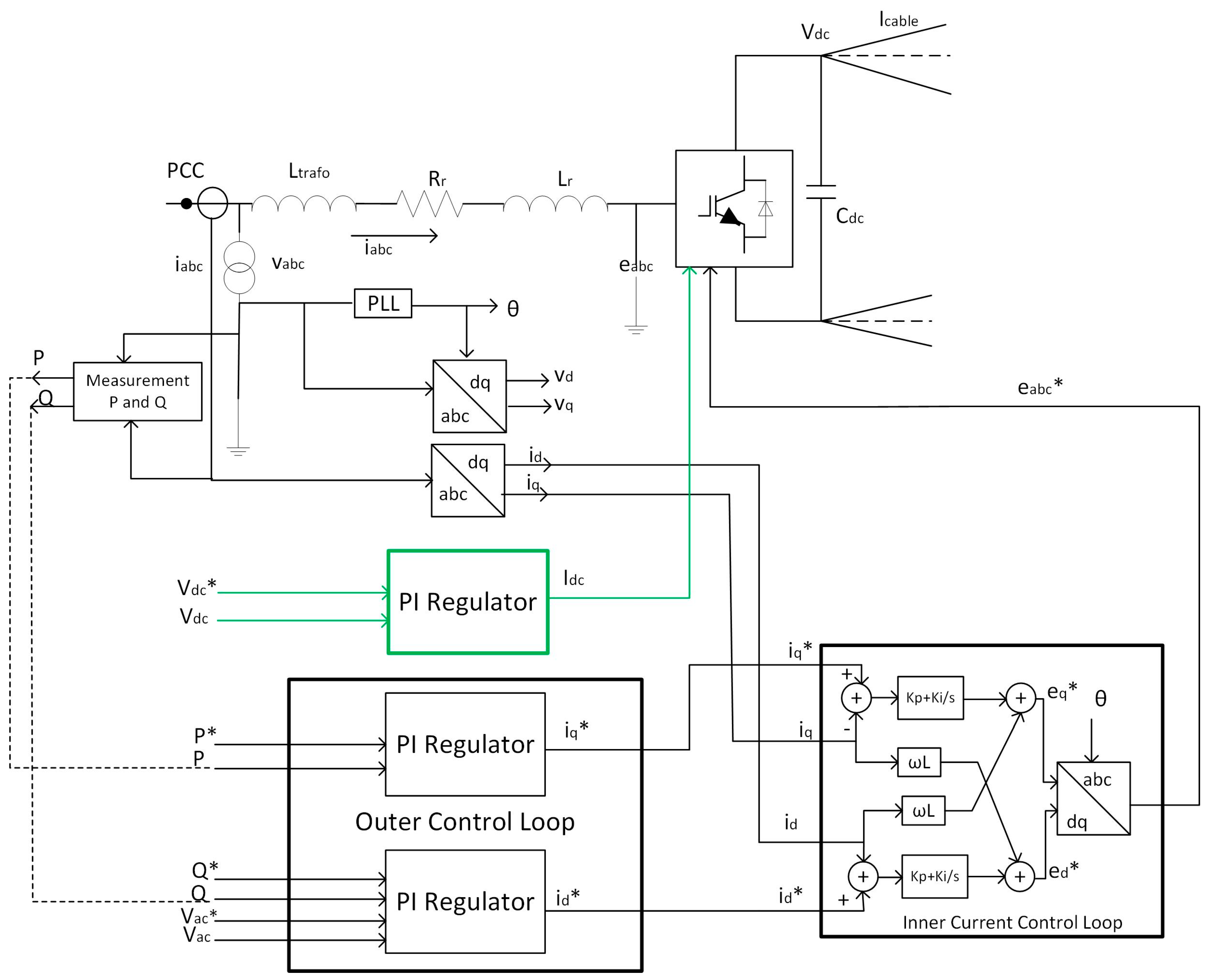
Figure 2.
Frequency dependent cable model with five parallel sections and three series branches.
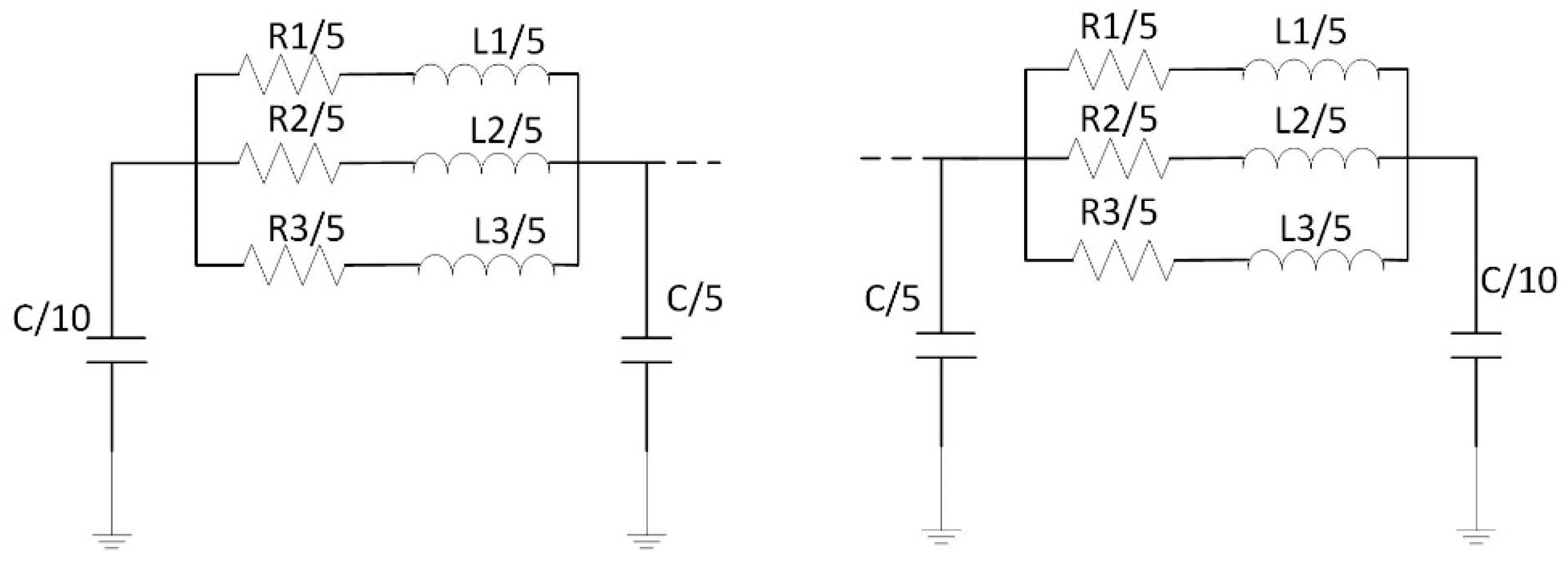
Figure 3.
Radial DC grid with three nodes.
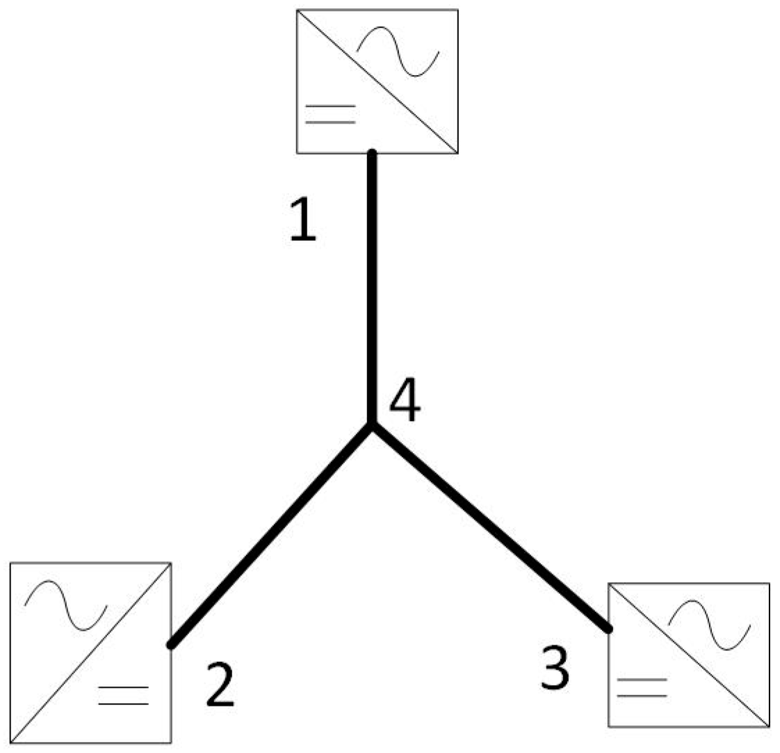
Figure 4.
Eigenvalues of the grid from Figure 3.
Figure 4.
Eigenvalues of the grid from Figure 3.

Figure 5.
Interaction modes of the grid from Figure 3.
Figure 5.
Interaction modes of the grid from Figure 3.
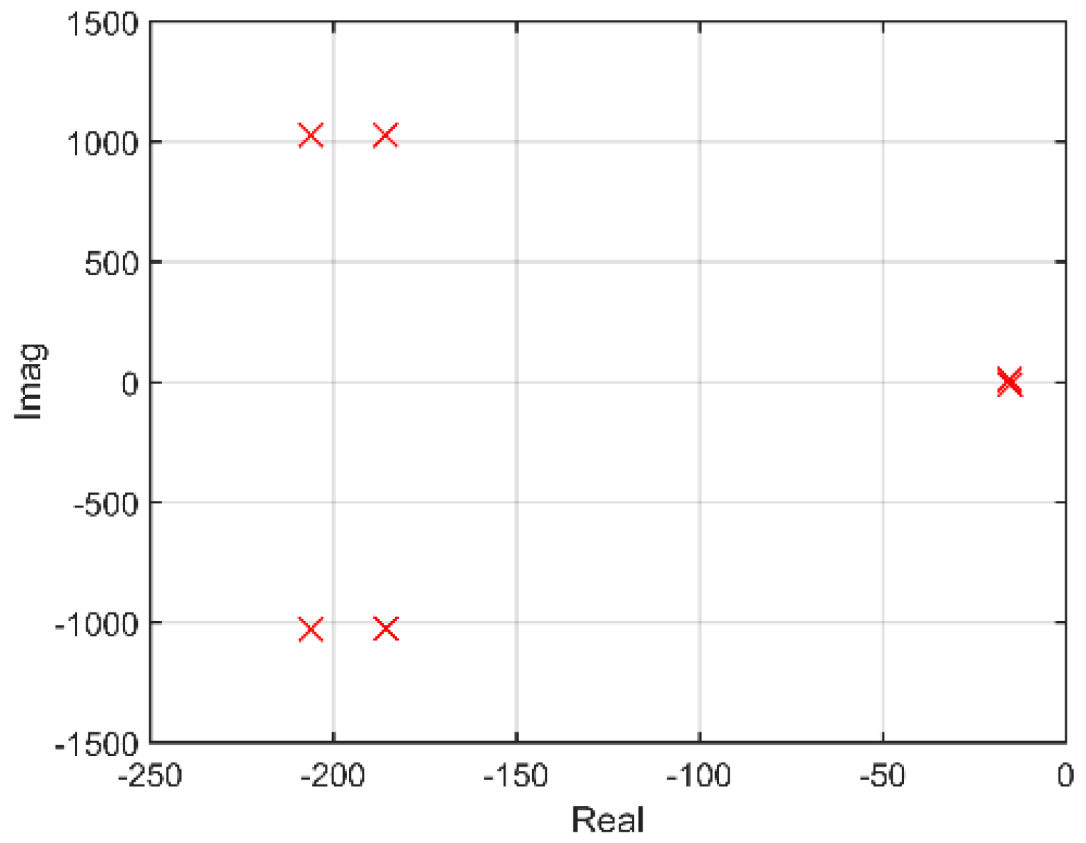
Figure 6.
Normalized participation factors of interaction modes: (a) Mode 1; (b) Mode 2; and (c) Mode 3.
Figure 6.
Normalized participation factors of interaction modes: (a) Mode 1; (b) Mode 2; and (c) Mode 3.

Figure 7.
Interaction modes (Case 4.1a): (a) all; and (b) zoom in of Mode 3.

Figure 8.
Time-domain simulations (Case 4.1a): (a) Direct voltage 1; (b) Direct voltages 2 and 3.
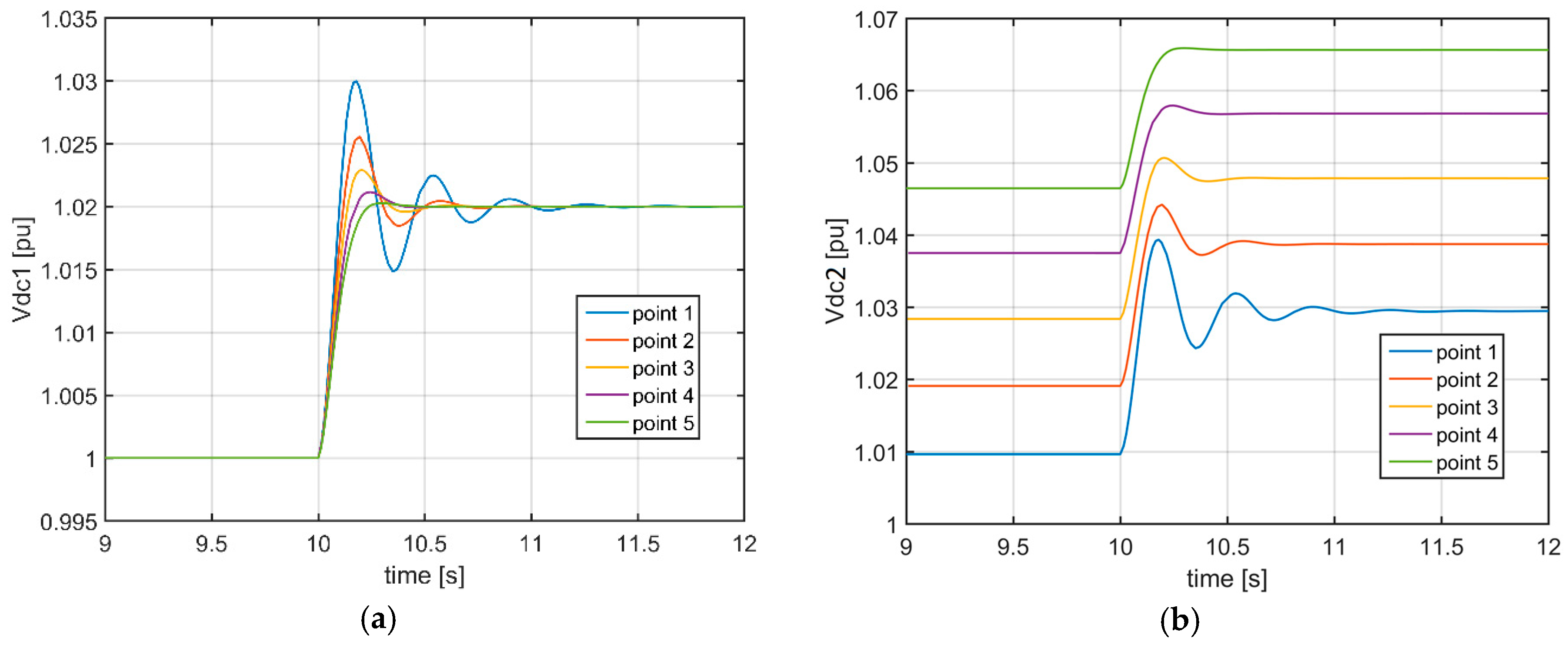
Figure 9.
Interaction modes (Case 4.1b).

Figure 10.
Interaction modes (Case 4.2): (a) all; and (b) zoom in of Mode 3.

Figure 11.
Damping factors of interaction modes (Case 4.3).
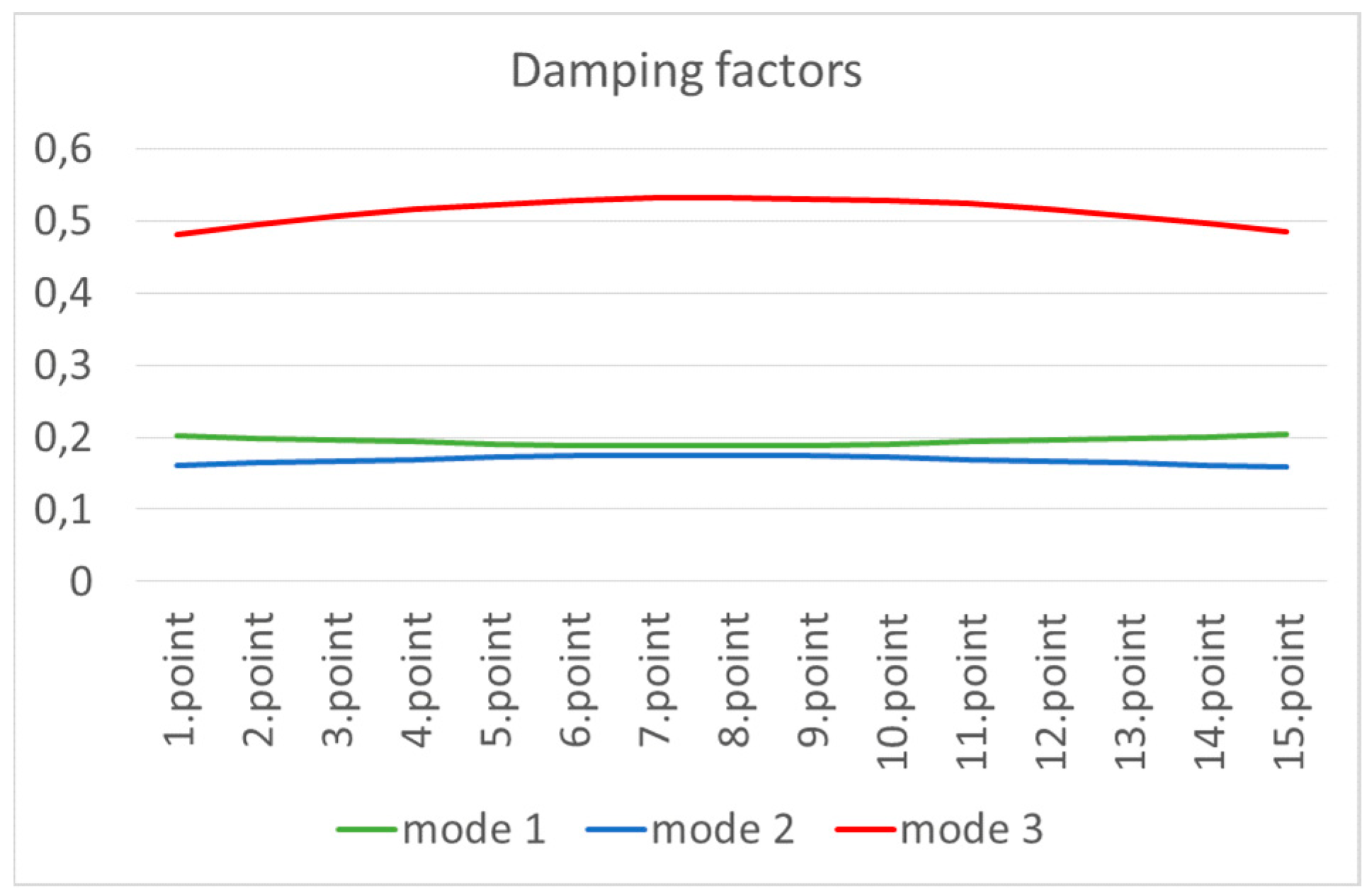
Figure 12.
Normalized participation factors of interaction modes (Case 4.3): (a) Mode 1; (b) Mode 2; and (c) Mode 3.
Figure 12.
Normalized participation factors of interaction modes (Case 4.3): (a) Mode 1; (b) Mode 2; and (c) Mode 3.
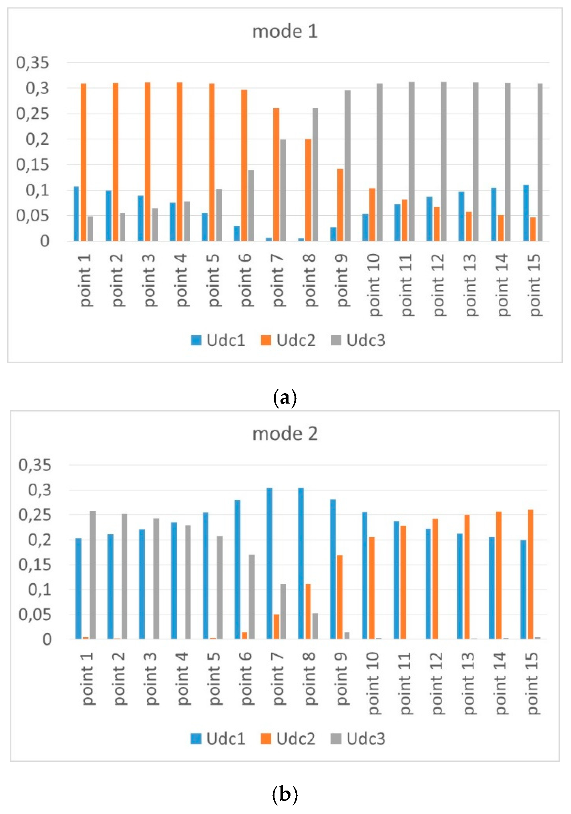
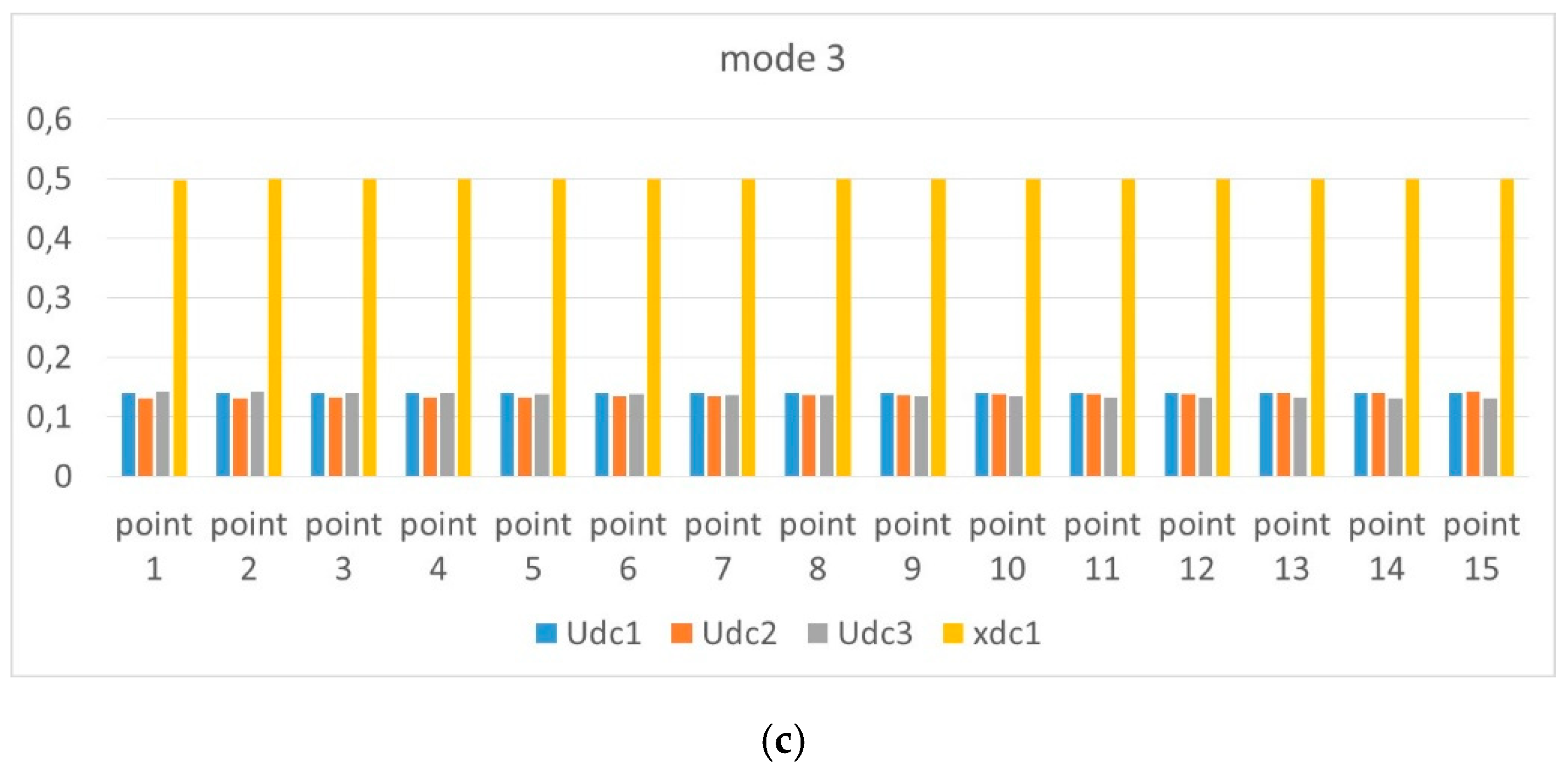
Figure 13.
Interaction modes (Case 4.4): (a) all; and (b) zoom in of Mode 3.
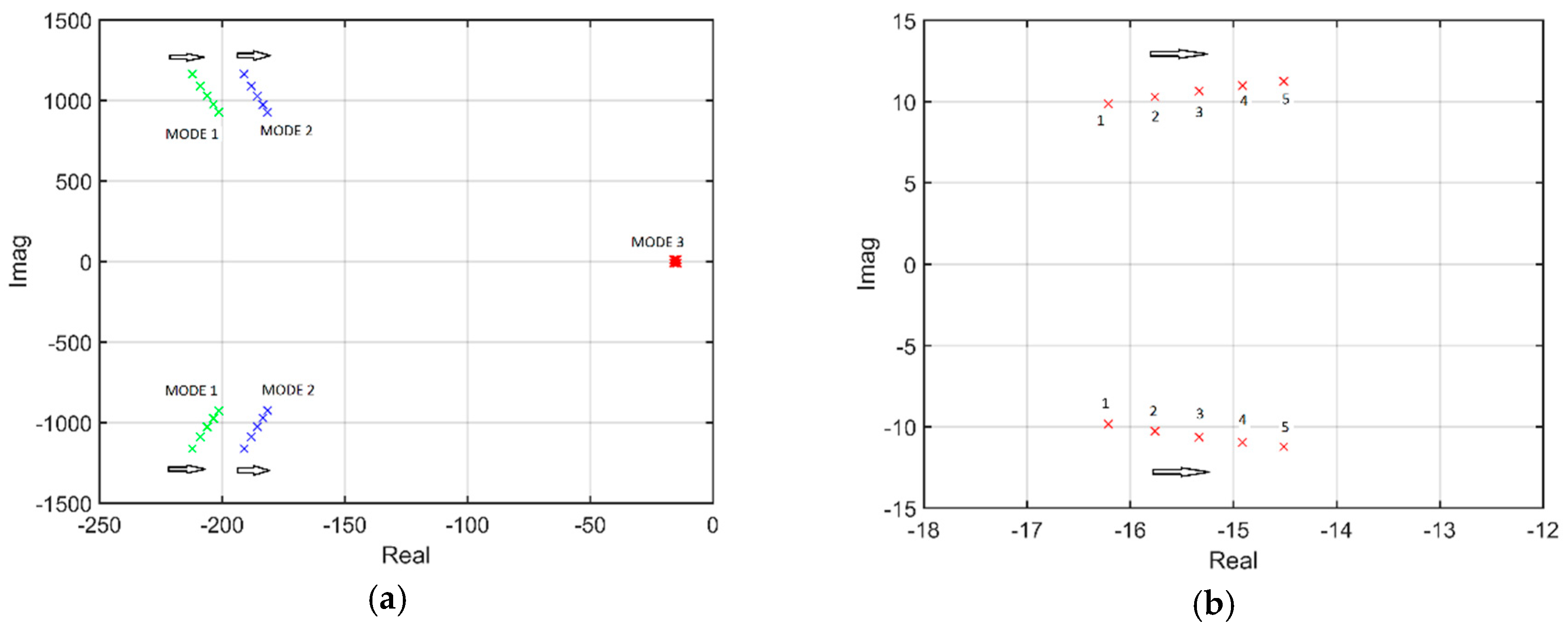
Figure 14.
Interaction modes (Case 4.5): (a) Mode 1 and Mode 2; and (b) Mode 3.
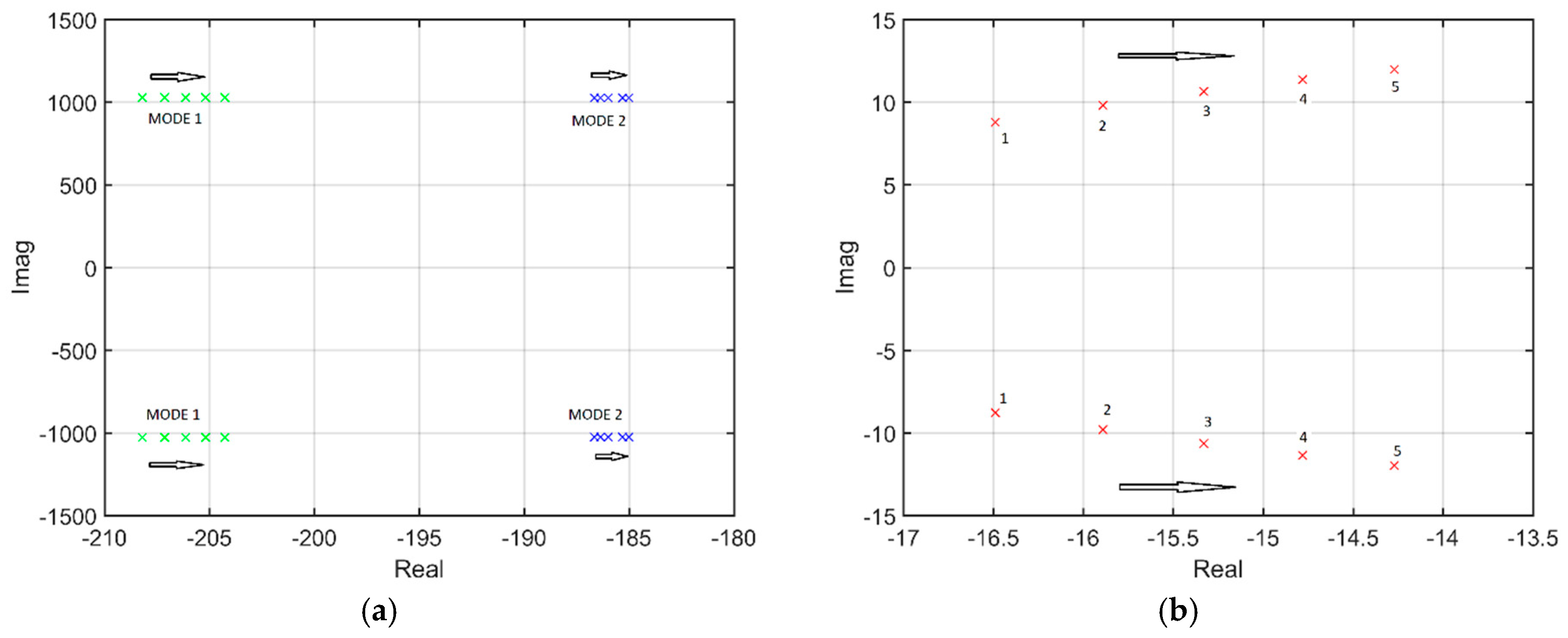
Figure 15.
Dominant interaction modes (Case 5.1).
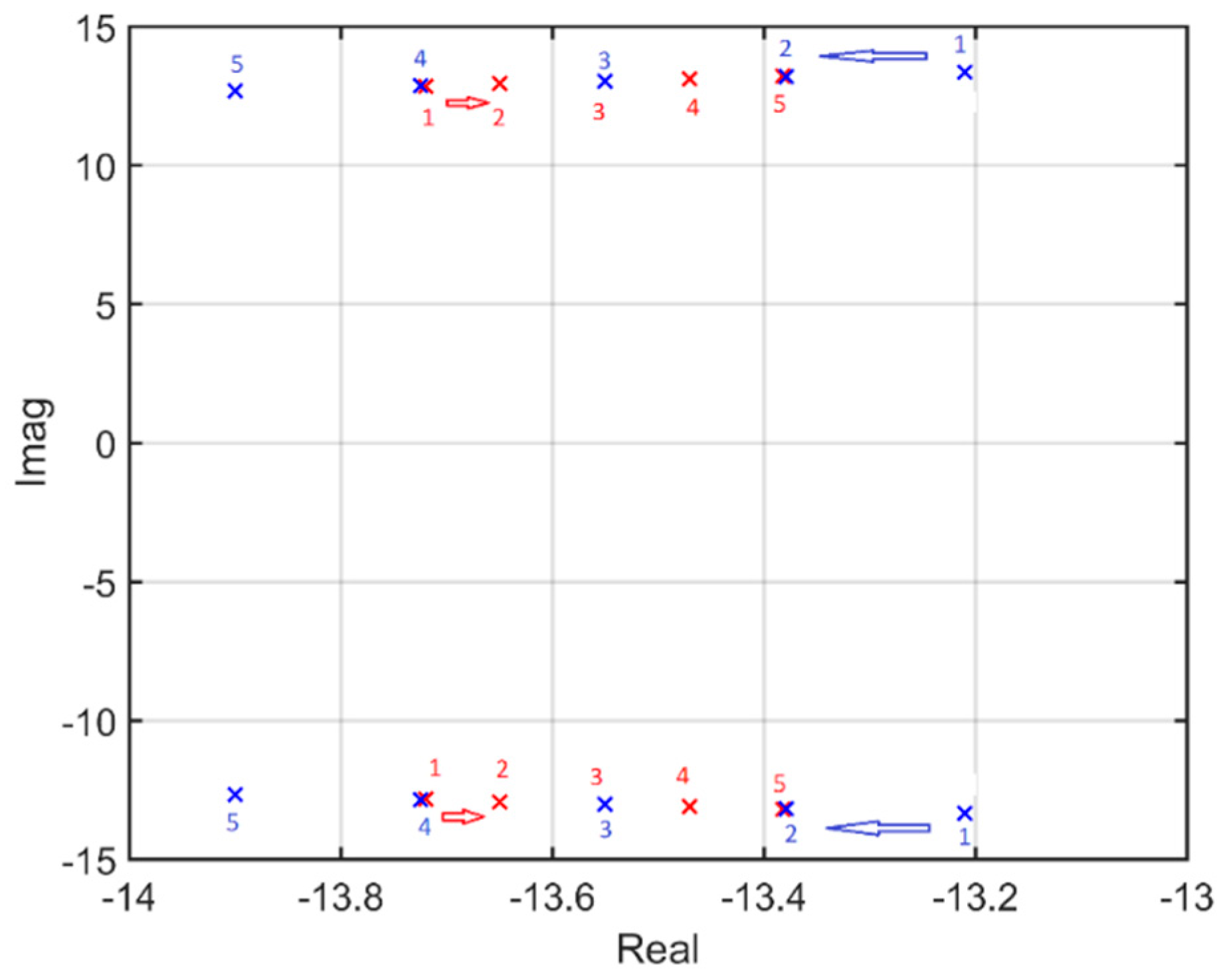
Figure 16.
Dominant interaction modes (Case 5.2).
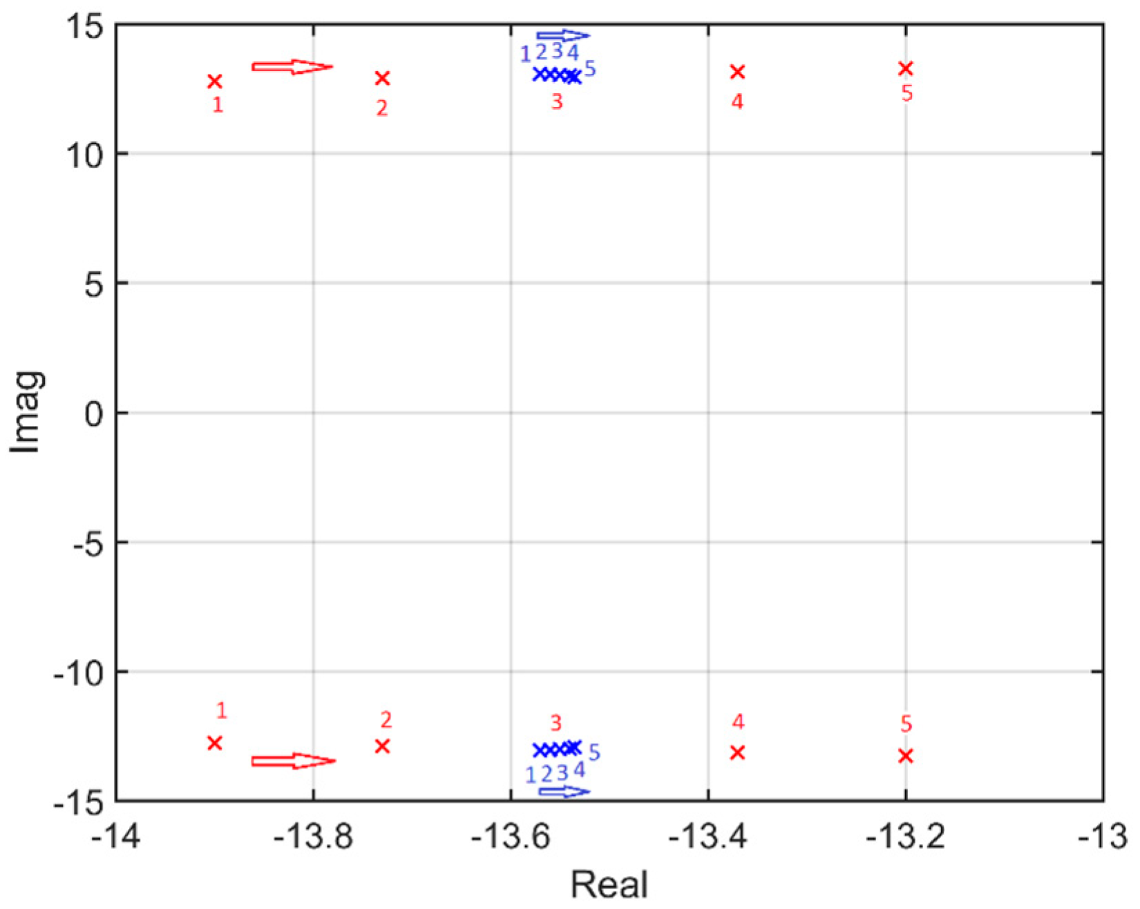
Figure 17.
Dominant interaction modes (Case 5.3).

Figure 18.
Points of equal currents and stability of dominant interaction modes (Case 5.3).
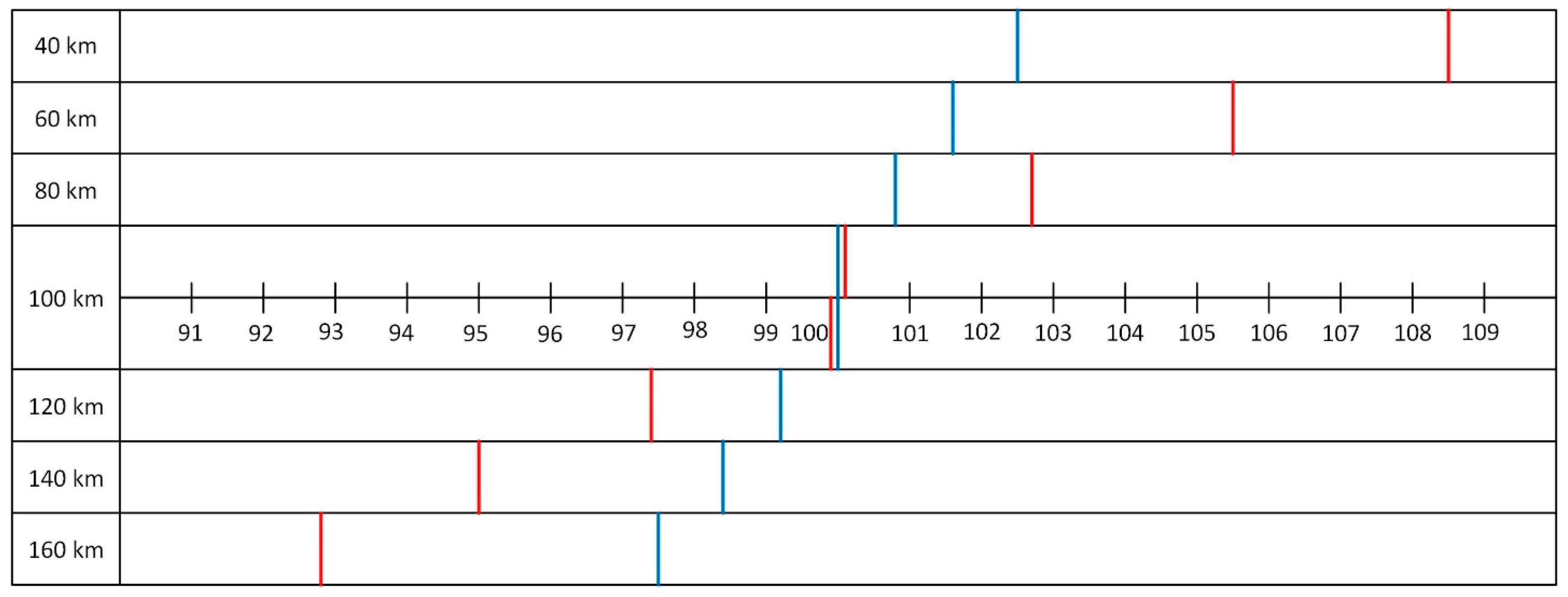
Figure 19.
Triangular DC grid.

Figure 20.
Radial DC grid with five nodes.

Table 1.
Converter powers and interaction modes (Case 4.1a).
| P1 [MW] | P2 [MW] | P3 [MW] | Mode 1 | ξ1 | Mode 2 | ξ2 | Mode 3 | ξ3 | |
|---|---|---|---|---|---|---|---|---|---|
| 1 | −19.80 | 10 | 10 | −185.40 ± 1025.2 j | 0.18 | −178.19 ± 1026.3 j | 0.17 | −3.39 ± 18.06 j | 0.18 |
| 2 | −39.23 | 20 | 20 | −190.76 ± 1026.0 j | 0.18 | −180.25 ± 1026.4 j | 0.17 | −6.55 ± 17.25 j | 0.35 |
| 3 | −58.29 | 30 | 30 | −196.04 ± 1026.7 j | 0.19 | −182.14 ± 1026.6 j | 0.17 | −9.58 ± 15.85 j | 0.52 |
| 4 | −77.02 | 40 | 40 | −201.16 ± 1027.3 j | 0.19 | −183.93 ± 1026.7 j | 0.18 | −12.51 ± 13.76 j | 0.67 |
| 5 | −95.42 | 50 | 50 | −206.13 ± 1027.9 j | 0.20 | −185.65 ± 1026.8 j | 0.18 | −15.33 ± 10.64 j | 0.82 |
Table 2.
Converter powers and interaction modes (Case 4.1b).
| P1 [MW] | P2 [MW] | P3 [MW] | Mode 1 | ξ1 | Mode 2 | ξ2 | Mode 3 | ξ3 | |
|---|---|---|---|---|---|---|---|---|---|
| 1 | −9.90 | 20 | −9.90 | −183.48 ± 1026.2 j | 0.18 | −176.23 ± 1024.6 j | 0.17 | −1.71 ± 18.25j | 0.09 |
| 2 | −19.62 | 40 | −19.62 | −190.20 ± 1027.1 j | 0.18 | −173.19 ± 1023.9 j | 0.17 | −3.18 ± 18.09j | 0.17 |
| 3 | −29.15 | 60 | −29.15 | −196.74 ± 1027.6 j | 0.19 | −170.16 ± 1023.3 j | 0.16 | −4.52 ± 17.84j | 0.25 |
| 4 | −38.50 | 80 | −38.50 | −203.10 ± 1027.9 j | 0.19 | −167.18 ± 1022.7 j | 0.16 | −5.74 ± 17.53j | 0.31 |
| 5 | −47.71 | 100 | −47.71 | −209.26 ± 1028.1 j | 0.20 | −164.25 ± 1022.1 j | 0.16 | −6.86 ± 17.16j | 0.37 |
Table 3.
Converter powers and interaction modes (Case 4.2).
| P1 [MW] | P2 [MW] | P3 [MW] | Mode 1 | ξ1 | Mode 2 | ξ2 | Mode 3 | ξ3 | |
|---|---|---|---|---|---|---|---|---|---|
| 1 | −7.96 | 60 | −50 | −195.97 ± 1027.6 j | 0.19 | −162.58 ± 1021.7 j | 0.16 | −0.77 ± 18.31 j | 0.04 |
| 2 | −18.20 | 60 | −40 | −196.28 ± 1027.6 j | 0.19 | −166.34 ± 1022.5 j | 0.16 | −2.60 ± 18.18 j | 0.14 |
| 3 | −28.29 | 60 | −30 | −196.70 ± 1027.6 j | 0.19 | −169.87 ± 1023.3 j | 0.16 | −4.37 ± 17.88 j | 0.24 |
| 4 | −38.24 | 60 | −20 | −197.27 ± 1027.6 j | 0.19 | −173.17 ± 1023.9 j | 0.17 | −6.08 ± 17.41 j | 0.33 |
| 5 | −48.07 | 60 | −10 | −198.02 ± 1027.6 j | 0.19 | −176.18 ± 1024.6 j | 0.17 | −7.73 ± 16.78 j | 0.42 |
| 6 | −57.76 | 60 | 0 | −199.01 ± 1027.6 j | 0.19 | −178.87 ± 1025.1 j | 0.17 | −9.34 ± 15.99 j | 0.50 |
| 7 | −67.34 | 60 | 10 | −200.29 ± 1027.7 j | 0.19 | −181.18 ± 1025.6 j | 0.17 | −10.90 ± 15.02 j | 0.59 |
| 8 | −76.79 | 60 | 20 | −201.90 ± 1027.8 j | 0.19 | −183.08 ± 1026.0 j | 0.18 | −12.41 ± 13.84 j | 0.67 |
| 9 | −86.13 | 60 | 30 | −203.81 ± 1027.9 j | 0.19 | −184.60 ± 1026.3 j | 0.18 | −13.88 ± 12.42 j | 0.75 |
| 10 | −95.37 | 60 | 40 | −206.00 ± 1028.1 j | 0.20 | −185.76 ± 1026.6 j | 0.18 | −15.30 ± 10.67 j | 0.82 |
Table 4.
Converter powers and interaction modes (Case 4.3).
| P1 [MW] | P2 [MW] | P3 [MW] | Mode 1 | ξ1 | Mode 2 | ξ2 | Mode 3 | ξ3 | |
|---|---|---|---|---|---|---|---|---|---|
| 1 | −60 | 105.1 | −40 | −211.18 ± 1028.2 j | 0.20 | −166.97 ± 1022.7 j | 0.16 | −8.89 ± 16.25 j | 0.48 |
| 2 | −60 | 94.2 | −30 | −208.15 ± 1028.2 j | 0.20 | −170.18 ± 1023.4 j | 0.16 | −9.15± 16.11 j | 0.49 |
| 3 | −60 | 83.5 | −20 | −205.23 ± 1028.1 j | 0.20 | −173.27 ± 1024.0 j | 0.17 | −9.37 ± 15.98 j | 0.51 |
| 4 | −60 | 72.9 | −10 | −202.42 ± 1027.9 j | 0.19 | −176.20 ± 1024.6 j | 0.17 | −9.55 ± 15.88 j | 0.52 |
| 5 | −60 | 62.4 | 0 | −199.82 ± 1027.7 j | 0.19 | −178.87 ± 1025.1 j | 0.17 | −9.68 ± 15.80 j | 0.52 |
| 6 | −60 | 52.1 | 10 | −197.69 ± 1027.4 j | 0.19 | −181.08 ± 1025.7 j | 0.17 | −9.78 ± 15.74 j | 0.53 |
| 7 | −60 | 41.9 | 20 | −196.40 ± 1027.1 j | 0.19 | −182.41 ± 1026.2 j | 0.18 | −9.83 ± 15.70 j | 0.53 |
| 8 | −60 | 31.8 | 30 | −196.43 ± 1026.8 j | 0.19 | −182.38 ± 1026.6 j | 0.18 | −9.85 ± 15.69 j | 0.53 |
| 9 | −60 | 21.85 | 40 | −197.75 ± 1026.7 j | 0.19 | −181.04 ± 102.6 j | 0.17 | −9.83 ± 15.70 j | 0.53 |
| 10 | −60 | 12 | 50 | −199.84 ± 1026.8 j | 0.19 | −178.90 ± 1026.4 j | 0.17 | −9.77 ± 15.74 j | 0.53 |
| 11 | −60 | 2.35 | 60 | −202.32 ± 1026.8 j | 0.19 | −176.37 ± 1026.1 j | 0.17 | −9.69 ± 15.79 j | 0.52 |
| 12 | −60 | −7.3 | 70 | −204.98 ± 1027.0 j | 0.20 | −173.60 ± 1025.7 j | 0.17 | −9.55 ± 15.88 j | 0.52 |
| 13 | −60 | −16.8 | 80 | −207.72 ± 1027.1 j | 0.20 | −170.72 ± 1025.3 j | 0.16 | −9.39 ± 15.98 j | 0.51 |
| 14 | −60 | −26.1 | 90 | −210.52 ± 1027.2 j | 0.20 | −167.80 ± 1024.8 j | 0.16 | −9.20 ± 16.09 j | 0.50 |
| 15 | −60 | −35.4 | 100 | −213.32 ± 1027.3 j | 0.20 | −164.81 ± 1024.2 j | 0.16 | −8.96 ± 16.22 j | 0.48 |
Table 5.
Line lengths, converter powers and interaction modes (Case 4.4).
| l1, l2, l3 [km] | P1 [MW] | P2 [MW] | P3 [MW] | Mode 1 | ξ1 | Mode 2 | ξ2 | Mode 3 | ξ3 | |
|---|---|---|---|---|---|---|---|---|---|---|
| 1 | 80 | −96.25 | 50 | 50 | −212.14 ± 1164.1 j | 0.18 | −191.00 ± 1163.2 j | 0.16 | −16.21 ± 9.85 j | 0.85 |
| 2 | 90 | −95.83 | 50 | 50 | −208.95 ± 1090.4 j | 0.19 | −188.15 ± 1089.3 j | 0.17 | −15.76 ± 10.27 j | 0.84 |
| 3 | 100 | −95.42 | 50 | 50 | −206.13 ± 1027.9 j | 0.20 | −185.65 ± 1026.8 j | 0.18 | −15.33 ± 10.64 j | 0.82 |
| 4 | 110 | −95.02 | 50 | 50 | −203.62 ± 974.1 j | 0.20 | −183.46 ± 972.9 j | 0.19 | −14.91 ± 10.97 j | 0.81 |
| 5 | 120 | −94.62 | 50 | 50 | −201.37 ± 927.1 j | 0.21 | −181.51 ± 925.8 j | 0.19 | −14.51 ± 11.25 j | 0.79 |
Table 6.
Referent voltages, converter powers and interaction modes (Case 4.5).
| Vdc1 [pu] | P1 [MW] | P2 [MW] | P3 [MW] | Mode 1 | ξ1 | Mode 2 | ξ2 | Mode 3 | ξ3 | |
|---|---|---|---|---|---|---|---|---|---|---|
| 1 | 0.96 | −95.08 | 50 | 50 | −208.20 ± 1028.1 j | 0.20 | −186.37 ± 1026.8 j | 0.18 | −16.49 ± 8.78 j | 0.88 |
| 2 | 0.98 | −95.25 | 50 | 50 | −207.14 ± 1028.0 j | 0.20 | −186.00 ± 1026.8 j | 0.18 | −15.89 ± 9.80 j | 0.85 |
| 3 | 1.00 | −95.42 | 50 | 50 | −206.13 ± 1027.9 j | 0.20 | −185.65 ± 1026.8 j | 0.18 | −15.33 ± 10.64 j | 0.82 |
| 4 | 1.02 | −95.58 | 50 | 50 | −205.18 ± 1027.8 j | 0.20 | −185.32 ± 1026.8 j | 0.18 | −14.78 ± 11.36 j | 0.79 |
| 5 | 1.04 | –95.73 | 50 | 50 | –204.27 ± 1027.7 j | 0.19 | –185.01 ± 1026.8 j | 0.18 | –14.27 ± 11.98 j | 0.77 |
Table 7.
Converter powers, voltages, currents and dominant interaction modes (Case 5.1).
| P1 [MW] | P2 [MW] | P3 [MW] | Vdc1 [pu] | Vdc2 [pu] | Vdc3 [pu] | Idc2 [pu] | Idc3 [pu] | Voltage Control 2 | Voltage Control 3 | |||
|---|---|---|---|---|---|---|---|---|---|---|---|---|
| λ | ξ | λ | ξ | |||||||||
| 1 | 222.72 | −100 | −98 | 1 | 0.8914 | 0.8921 | 0.5609 | 0.5493 | −13.72 ± 12.85 j | 0.7298 | −13.21 ± 13.36 j | 0.7031 |
| 2 | 224.01 | −100 | −99 | 1 | 0.8909 | 0.8913 | 0.5612 | 0.5554 | −13.65 ± 12.94 j | 0.7257 | −13.38 ± 13.20 j | 0.7119 |
| 3 | 225.29 | −100 | −100 | 1 | 0.8905 | 0.8905 | 0.5615 | 0.5615 | −13.55 ± 13.03 j | 0.7208 | −13.55 ± 13.03 j | 0.7208 |
| 4 | 226.58 | −100 | −101 | 1 | 0.8901 | 0.8897 | 0.5617 | 0.5676 | −13.47 ± 13.11 j | 0.7166 | −13.72 ± 12.85 j | 0.7299 |
| 5 | 227.87 | −100 | −102 | 1 | 0.8896 | 0.8889 | 0.5621 | 0.5737 | −13.38 ± 13.20 j | 0.7119 | −13.90 ± 12.67 j | 0.7390 |
Table 8.
Line lengths, converter powers, voltages, currents and dominant interaction modes (Case 5.2).
Table 8.
Line lengths, converter powers, voltages, currents and dominant interaction modes (Case 5.2).
| L3 [km] | P1 [MW] | P2 [MW] | P3 [MW] | Vdc1 [pu] | Vdc2 [pu] | Vdc2 [pu] | Idc2 [pu] | Idc3 [pu] | Voltage Control 2 | Voltage Control 3 | |||
|---|---|---|---|---|---|---|---|---|---|---|---|---|---|
| λ | ξ | λ | ξ | ||||||||||
| 1 | 90 | 224.77 | −100 | −100 | 1 | 0.8907 | 0.8945 | 0.5614 | 0.5590 | −13.90 ± 12.78 j | 0.7361 | −13.57 ± 13.07 j | 0.7203 |
| 2 | 95 | 225.03 | −100 | −100 | 1 | 0.8906 | 0.8925 | 0.5614 | 0.5602 | −13.73 ± 12.91 j | 0.7285 | −13.56 ± 13.05 j | 0.7205 |
| 3 | 100 | 225.29 | −100 | −100 | 1 | 0.8905 | 0.8905 | 0.5615 | 0.5615 | −13.55 ± 13.03 j | 0.7208 | −13.55 ± 13.03 j | 0.7208 |
| 4 | 105 | 225.56 | −100 | −100 | 1 | 0.8904 | 0.8885 | 0.5615 | 0.5627 | −13.37 ± 13.14 j | 0.7132 | −13.54 ± 13.01 j | 0.7211 |
| 5 | 110 | 225.82 | −100 | −100 | 1 | 0.8903 | 0.8865 | 0.5616 | 0.5640 | −13.20 ± 13.26 j | 0.7055 | −13.54 ± 12.94 j | 0.7229 |
Table 9.
Converter powers, voltages, currents and dominant interaction modes (Case 5.3).
| P1 [MW] | P2 [MW] | P3 [MW] | Vdc1 [pu] | Vdc2 [pu] | Vdc3 [pu] | Idc2 [pu] | Idc3 [pu] | Voltage Control 2 | Voltage Control 3 | |||
|---|---|---|---|---|---|---|---|---|---|---|---|---|
| λ | ξ | λ | ξ | |||||||||
| 1 | 223.26 | −100 | −100 | 1 | 0.8912 | 0.9061 | 0.5610 | 0.5518 | −14.93 ± 11.99 j | 0.7797 | −13.62 ± 13.19 j | 0.7184 |
| 2 | 224.50 | −100 | −101 | 1 | 0.8908 | 0.9055 | 0.5613 | 0.5577 | −14.87 ± 12.07 j | 0.7764 | −13.80 ± 13.02 j | 0.7274 |
| 3 | 225.74 | −100 | −102 | 1 | 0.8904 | 0.9049 | 0.5615 | 0.5636 | −14.80 ± 12.16 j | 0.7727 | −13.97 ± 12.84 j | 0.7363 |
| 4 | 226.99 | −100 | −103 | 1 | 0.8899 | 0.9042 | 0.5619 | 0.5696 | −14.74 ± 12.24 j | 0.7693 | −14.14 ± 12.66 j | 0.7450 |
| 5 | 228.24 | −100 | −104 | 1 | 0.8895 | 0.9036 | 0.5621 | 0.5755 | −14.67 ± 12.32 j | 0.7658 | −14.31 ± 12.47 j | 0.7539 |
| 6 | 229.49 | −100 | −105 | 1 | 0.8892 | 0.9030 | 0.5623 | 0.5814 | −14.60 ± 12.41 j | 0.7619 | −14.48 ± 12.28 j | 0.7627 |
| 7 | 230.74 | −100 | −106 | 1 | 0.8887 | 0.9023 | 0.5626 | 0.5874 | −14.54 ± 12.49 j | 0.7586 | −14.65 ± 12.08 j | 0.7715 |
Table 10.
Converter powers, voltages, currents and dominant interaction modes (Case 5.4.1).
| P1 [MW] | P2 [MW] | P3 [MW] | Vdc1 [pu] | Vdc2 [pu] | Vdc3 [pu] | Idc2 [pu] | Idc3 [pu] | Voltage Control 2 | Voltage Control 3 | |||
|---|---|---|---|---|---|---|---|---|---|---|---|---|
| λ | ξ | λ | ξ | |||||||||
| 1 | 222.72 | −100 | −98 | 1 | 0.8914 | 0.8921 | 0.5609 | 0.5493 | −10.26 ± 12.58 j | 0.6320 | −9.88 ± 12.87 j | 0.6089 |
| 2 | 224.01 | −100 | −99 | 1 | 0.8909 | 0.8913 | 0.5612 | 0.5554 | −10.20 ± 12.63 j | 0.6283 | −10.00 ± 12.77 j | 0.6165 |
| 3 | 225.29 | −100 | −100 | 1 | 0.8905 | 0.8905 | 0.5615 | 0.5615 | −10.13 ± 12.68 j | 0.6242 | −10.13 ± 12.68 j | 0.6242 |
| 4 | 226.58 | −100 | −101 | 1 | 0.8901 | 0.8897 | 0.5617 | 0.5676 | −10.07 ± 12.73 j | 0.6204 | −10.26 ± 12.58 j | 0.6320 |
| 5 | 227.87 | – | – | 1 | 0.8896 | 0.8889 | 0.5621 | 0.5737 | −10.00 ± 12.78 j | 0.6162 | −10.39 ± 12.48 j | 0.6398 |
Table 11.
Line length, power of converters, voltages, currents and dominant interaction modes (Case 5.4.2).
Table 11.
Line length, power of converters, voltages, currents and dominant interaction modes (Case 5.4.2).
| L12 [km] | L13 [km] | L23 [km] | P1 [MW] | P2 [MW] | P3 [MW] | Vdc1 [pu] | Vdc2 [pu] | Vdc2 [pu] | Idc2 [pu] | Idc3 [pu] | Voltage Control 2 | Voltage Control 3 | |||
|---|---|---|---|---|---|---|---|---|---|---|---|---|---|---|---|
| λ | ξ | λ | ξ | ||||||||||||
| 1 | 311.11 | 280 | 280 | 224.77 | −100 | −100 | 1 | 0.8907 | 0.8945 | 0.5614 | 0.5590 | −10.47 ± 12.58 j | 0.6397 | −10.21 ± 12.73 j | 0.6257 |
| 2 | 205.26 | 290 | 290 | 225.03 | −100 | −100 | 1 | 0.8906 | 0.8925 | 0.5614 | 0.5602 | −10.30 ± 12.63 j | 0.6320 | −10.17 ± 12.70 j | 0.6251 |
| 3 | 300 | 300 | 300 | 225.29 | −100 | −100 | 1 | 0.8905 | 0.8905 | 0.5615 | 0.5615 | −10.13 ± 12.68 j | 0.6242 | −10.13 ± 12.68 j | 0.6242 |
| 4 | 295.24 | 310 | 310 | 225.56 | −100 | −100 | 1 | 0.8904 | 0.8885 | 0.5615 | 0.5627 | −9.96 ± 12.72 j | 0.6165 | −10.09 ± 12.65 j | 0.6236 |
| 5 | 290.91 | 320 | 320 | 225.82 | −100 | −100 | 1 | 0.8903 | 0.8865 | 0.5616 | 0.5640 | −9.79 ± 12.76 j | 0.6087 | −10.05 ± 12.62 j | 0.6230 |
Table 12.
Converter powers, voltages, currents and dominant interaction modes (Case 5.3).
| P1 [MW] | P2 [MW] | P3 [MW] | Vdc1 [pu] | Vdc2 [pu] | Vdc3 [pu] | Idc2 [pu] | Idc3 [pu] | Voltage Control 2 | Voltage Control 3 | |||
|---|---|---|---|---|---|---|---|---|---|---|---|---|
| λ | ξ | λ | ξ | |||||||||
| 1 | 223.26 | −100 | −100 | 1 | 0.8912 | 0.9061 | 0.5610 | 0.5518 | −11.38 ± 12.22 j | 0.6815 | −10.36 ± 12.86 j | 0.6273 |
| 2 | 224.50 | −100 | −101 | 1 | 0.8908 | 0.9055 | 0.5613 | 0.5577 | −11.33 ± 12.27 j | 0.6784 | −10.49 ± 12.76 j | 0.6350 |
| 3 | 225.74 | −100 | −102 | 1 | 0.804 | 0.9049 | 0.5615 | 0.5636 | −11.28 ± 12.32 j | 0.6753 | −10.62 ± 12.66 j | 0.6427 |
| 4 | 226.99 | −100 | −103 | 1 | 0.8899 | 0.9042 | 0.5619 | 0.5696 | −11.23 ± 12.37 j | 0.6722 | −10.75 ± 12.55 j | 0.6505 |
| 5 | 228.24 | −100 | −104 | 1 | 0.8895 | 0.9036 | 0.5621 | 0.5755 | −11.18 ± 12.41 j | 0.6693 | −10.88 ± 12.44 j | 0.6583 |
| 6 | 229.49 | −100 | −105 | 1 | 0.8892 | 0.9030 | 0.5623 | 0.5814 | −11.13 ± 12.46 j | 0.6662 | −11.01 ± 12.33 j | 0.6661 |
| 7 | 230.74 | −100 | −106 | 1 | 0.8887 | 0.9023 | 0.5626 | 0.5874 | −11.07 ± 12.51 j | 0.6627 | −11.14 ± 12.22 j | 0.6737 |
Table 13.
Line lengths, converter powers, voltages, currents and dominant interaction modes (Case 5.5.1).
Table 13.
Line lengths, converter powers, voltages, currents and dominant interaction modes (Case 5.5.1).
| Converter | L [km] | P [MW] | Vdc [pu] | Idc [pu] | λ |
|---|---|---|---|---|---|
| Converter 1 | 20 | 203.86 | 1 | 1.0193 | — |
| Converter 2 | 20 | −50 | 0.9794 | 0.2553 | −4.88 ± 14.71 j |
| Converter 3 | 20 | −60 | 0.9787 | 0.3065 | −6.15 ± 14.23 j |
| Converter 4 | 20 | −70 | 0.9781 | 0.3578 | −7.43 ± 13.61 j |
| Converter 5 | 20 | −80 | 0.9774 | 0.4092 | −8.71 ± 12.86 j |
Table 14.
Line lengths, converter powers, voltages, currents and dominant interaction modes (Case 5.5.2).
Table 14.
Line lengths, converter powers, voltages, currents and dominant interaction modes (Case 5.5.2).
| Converter | L [km] | P [MW] | Vdc [pu] | Idc [pu] | λ |
|---|---|---|---|---|---|
| Converter 1 | 20 | 204.93 | 1 | 1.0247 | — |
| Converter 2 | 20 | −50 | 0.9834 | 0.2542 | −4.82 ± 14.21 j |
| Converter 3 | 40 | −50 | 0.9801 | 0.2551 | −4.91 ± 14.21 j |
| Converter 4 | 60 | −50 | 0.9767 | 0.2560 | −5.00 ± 14.21 j |
| Converter 5 | 80 | −50 | 0.9734 | 0.2568 | −5.09 ± 14.21 j |
Table 15.
Line lengths, converter powers, voltages, currents and dominant interaction modes (Case 5.5.3).
Table 15.
Line lengths, converter powers, voltages, currents and dominant interaction modes (Case 5.5.3).
| Converter | L [km] | P [MW] | Vdc [pu] | Idc [pu] | λ |
|---|---|---|---|---|---|
| Converter 1 | 20 | 205.45 | 1 | 1.0273 | — |
| Converter 2 | 20 | −50.5 | 0.9833 | 0.2568 | −4.88 ± 14.19 j |
| Converter 3 | 40 | −50 | 0.9801 | 0.2551 | −4.91 ± 14.21 j |
| Converter 4 | 60 | −50 | 0.9767 | 0.2560 | −5.00 ± 14.21 j |
| Converter 5 | 80 | −50 | 0.9733 | 0.2569 | −5.09 ± 14.21 j |
Table 16.
Droop coefficients and dominant interaction modes (Case 5.5.4).
| g2 | g3 | g4 | g5 | λ | ξ | |
|---|---|---|---|---|---|---|
| 1. | 0.1 | 0.5 | 1 | 2.5 | −1.2486 ± 22.4053 j | 0.0556 |
| 2. | 0.1 | 0.5 | 2.5 | 1 | −1.2476 ± 22.4114 j | 0.0556 |
| 3. | 0.1 | 1 | 0.5 | 2.5 | −1.2395 ± 22.3679 j | 0.0553 |
| 4. | 0.1 | 1 | 2.5 | 0.5 | −1.2382 ± 22.3761 j | 0.0553 |
| 5. | 0.1 | 2.5 | 0.5 | 1 | −1.2102 ± 22.2620 j | 0.0543 |
| 6. | 0.1 | 2.5 | 1 | 0.5 | −1.2098 ± 22.2641 j | 0.0543 |
| 7. | 0.5 | 0.1 | 1 | 2.5 | −1.2413 ± 22.3735 j | 0.0554 |
| 8. | 0.5 | 0.1 | 2.5 | 1 | −1.2404 ± 22.3796 j | 0.0553 |
| 9. | 0.5 | 1 | 0.1 | 2.5 | −1.2248 ± 22.3061 j | 0.0548 |
| 10. | 0.5 | 1 | 2.5 | 0.1 | −1.2233 ± 22.3158 j | 0.0547 |
| 11. | 0.5 | 2.5 | 0.1 | 1 | −1.1953 ± 22.1999 j | 0.0538 |
| 12. | 0.5 | 2.5 | 1 | 0.1 | −1.1947 ± 22.2036 j | 0.0537 |
| 13. | 1 | 0.1 | 0.5 | 2.5 | −1.2228 ± 22.2962 j | 0.0548 |
| 14. | 1 | 0.1 | 2.5 | 0.5 | −1.2215 ± 22.3044 j | 0.0547 |
| 15. | 1 | 0.5 | 0.1 | 2.5 | −1.2154 ± 22.2662 j | 0.0545 |
| 16. | 1 | 0.5 | 2.5 | 0.1 | −1.2139 ± 22.2760 j | 0.0544 |
| 17. | 1 | 2.5 | 0.1 | 0.5 | −1.1760 ± 22.1243 j | 0.0531 |
| 18. | 1 | 2.5 | 0.5 | 0.1 | −1.1757 ± 22.1259 j | 0.0531 |
| 19. | 2.5 | 0.1 | 0.5 | 1 | −1.1631 ± 22.0703 j | 0.0526 |
| 20. | 2.5 | 0.1 | 1 | 0.5 | −1.1628 ± 22.0724 j | 0.0526 |
| 21. | 2.5 | 0.5 | 0.1 | 1 | −1.1555 ± 22.0401 j | 0.0524 |
| 22. | 2.5 | 0.5 | 1 | 0.1 | −1.1550 ± 22.0437 j | 0.0523 |
| 23. | 2.5 | 1 | 0.1 | 0.5 | −1.1456 ± 22.0043 j | 0.0520 |
| 24. | 2.5 | 1 | 0.5 | 0.1 | −1.1454 ± 22.0059 j | 0.0520 |
© 2017 by the authors. Licensee MDPI, Basel, Switzerland. This article is an open access article distributed under the terms and conditions of the Creative Commons Attribution (CC BY) license (http://creativecommons.org/licenses/by/4.0/).
Share and Cite
MDPI and ACS Style
Grdenić, G.; Delimar, M. Small-Signal Stability Analysis of Interaction Modes in VSC MTDC Systems with Voltage Margin Control. Energies 2017, 10, 873. https://doi.org/10.3390/en10070873
AMA Style
Grdenić G, Delimar M. Small-Signal Stability Analysis of Interaction Modes in VSC MTDC Systems with Voltage Margin Control. Energies. 2017; 10(7):873. https://doi.org/10.3390/en10070873
Chicago/Turabian StyleGrdenić, Goran, and Marko Delimar. 2017. "Small-Signal Stability Analysis of Interaction Modes in VSC MTDC Systems with Voltage Margin Control" Energies 10, no. 7: 873. https://doi.org/10.3390/en10070873
Note that from the first issue of 2016, this journal uses article numbers instead of page numbers. See further details here.