
A New Miniature Wind Turbine for Wind Tunnel Experiments. Part I: Design and Performance


Wind Engineering and Renewable Energy Laboratory (WIRE), École Polytechnique Fédérale de Lausanne (EPFL), EPFL-ENAC-IIE-WIRE, Lausanne 1015, Switzerland
*
Author to whom correspondence should be addressed.
Energies 2017, 10(7), 908; https://doi.org/10.3390/en10070908
Submission received: 10 May 2017
/
Revised: 24 June 2017
/
Accepted: 28 June 2017
/
Published: 3 July 2017
(This article belongs to the Collection Wind Turbines)
Abstract
:Miniature wind turbines, employed in wind tunnel experiments to study the interaction of turbines with turbulent boundary layers, usually suffer from poor performance with respect to their large-scale counterparts in the field. Moreover, although wakes of wind turbines have been extensively examined in wind tunnel studies, the proper characterization of the performance of wind turbines has received relatively less attention. In this regard, the present study concerns the design and the performance analysis of a new three-bladed horizontal-axis miniature wind turbine with a rotor diameter of 15 cm. Due to its small size, this turbine, called WiRE-01, is particularly suitable for studies of wind farm flows and the interaction of the turbine with an incoming boundary-layer flow. Especial emphasis was placed on the accurate measurement of the mechanical power extracted by the miniature turbine from the incoming wind. In order to do so, a new setup was developed to directly measure the torque of the rotor shaft. Moreover, to provide a better understanding on the connection between the mechanical and electrical aspects of miniature wind turbines, the performance of three different direct-current (DC) generators was studied. It is found that electrical outputs of the tested generators can be used to provide a rather acceptable estimation of the mechanical input power. Force and power measurements showed that the thrust and power coefficients of the miniature turbine can reach and , respectively, which are close to the ones of large-scale turbines in the field. In Part II of this study, the wake structure and dynamic flow characteristics are studied for the new miniature turbine immersed in a turbulent boundary-layer flow.
1. Introduction
Wind tunnel experiments have become an increasingly valuable tool to elucidate the performance of wind turbines and their wake characteristics [1]. A deep understanding of the wind turbine interaction with the atmospheric boundary layer (ABL) is essential as wind turbines operate in the ABL flow. Due to the unsteady nature of the ABL flow, wind turbines are subject to different incoming flow conditions (e.g., different wind direction and magnitude). Different scenarios of the ABL interaction with wind turbines can be simulated in a wind tunnel under fully controlled conditions. Additionally, as many wind turbines in wind farms have to operate in the wakes of upwind turbines, the study of the cumulative effects of turbine wakes in wind farms is of great importance. This goal can be achieved by performing wind tunnel simulations of the flow field in wind farms consisting of miniature wind turbines. Moreover, the usefulness of techniques to optimize the power production of the whole wind farm (e.g., yaw and pitch angle controls) can be first examined experimentally in wind tunnels.
In the light of the above-mentioned benefits of wind tunnel experiments, they have been widely used in the wind-energy community to study wind turbines and their wakes (e.g., [2,3,4,5,6,7,8,9,10,11,12,13,14,15,16,17,18,19,20,21]). However, there are still some open issues that need to be addressed in order to improve the suitability of wind tunnel studies of wind turbines. Due to the inevitable difference between the Reynolds number of the wind tunnel flow and the ABL one, miniature wind turbines usually have a poor performance compared to their large-scale counterparts. In general, the performance of a wind turbine is quantified through the definition of the normalized thrust force, called thrust coefficient , and the normalized power, called power coefficient . They are given by
where T is the total thrust force exerted on the turbine by the incoming wind, P is the power extracted by the turbine from the incoming wind, is the air density, d is the rotor diameter and is the mean streamwise incoming velocity at hub height. The overbar denotes temporal averaging. The value of reflects the ability of the turbine to extract power, and the overall strength of the turbine wake is determined by the value of [22]. Although some of the wind-tunnel studies in the literature (e.g., [23,24]) have tried to optimize the performance of miniature turbines, in general, values of and in most of the prior wind-tunnel studies of turbine wakes under boundary-layer inflow conditions are much lower than those of large-scale turbines. This calls for a better design of miniature turbines in order to attain more realistic values of and .
Another remaining challenge for wind tunnel studies of wind turbines concerns the accurate measurement of the wind turbine performance. As an example, the magnitude of the turbine extracted power for a miniature turbine with cm and ms is smaller than W, which makes it difficult to measure accurately. The extracted power (i.e., mechanical power ) for a turbine can be expressed as a product of the shaft torque and the rotational velocity of the rotor . This mechanical power is then converted to the electrical power in the generator attached to the rotor. The shaft torque of model turbines with relatively big rotor diameters ( cm) has been directly measured in former wind-tunnel studies (e.g., [25,26]). However, to our best knowledge, only a few studies in the literature have tried to directly measure the shaft torque of smaller miniature turbines, designed to study the interaction of turbines with turbulent boundary layers. This is due to low values of the shaft torque and also space limitations. Kang and Meneveau [27] measured the torque by mounting the generator inside a cylindrical housing with internal ball bearings where the rotation of the generator is prevented by the deflection of a strain-gauge sensor. Later, Howard et al. [28] used a similar concept to measure the mechanical torque. Instead of using a strain-gauge sensor, they measured the torque by adding known weights to the customized moment arm attached to the generator. In spite of the merit of these studies, the calibration procedure of these methods is rather cumbersome and they cannot be easily applied to different operating conditions.
Some previous studies (e.g., [29]) used to characterize the wind turbine performance as it can be easily measured. The value of is, however, smaller than due to the mechanical and electrical losses in the generator. More importantly, as the electrical power is affected by the characteristics of the generator [27], it will be shown later that the use of electrical power can lead to misleading information about the performance of the wind turbine. Some other studies (e.g., [18,19,30,31]), instead, benefited from known equations of direct-current (DC) generators to estimate the mechanical power from the electrical outputs. However, Kang and Meneveau [27] questioned the validity of this method. Therefore, it is unclear whether this method can reliably estimate the turbine mechanical power.
Overall, it seems that the power characterization of miniature turbines, as an interdisciplinary problem, suffers from a gap between the fluid mechanical aspect (i.e., the aerodynamic rotor performance) and the electrical one (i.e., DC-generator characteristics). The purpose of this paper is to design and fully test a new generation of miniature wind turbines, more representative of large-scale turbines in the field. The new miniature turbine is suitable for wind tunnel experiments which aim at studying the ABL interaction with wind turbines as well as turbine interactions with each other within wind farms. The wind turbine performance is characterized for different operating conditions. In particular, a new setup is developed to directly measure the torque of the rotor shaft under different operating conditions. Moreover, the paper provides a better understanding on the performance of DC generators in order to bridge the knowledge gap between the aerodynamic and electrical aspects of a wind turbine. The remainder of this paper is divided into three sections. In Section 2, the design of the miniature turbine is elaborated. The characterization of the wind turbine performance, including direct torque measurements, is given in Section 3. Finally, a summary is presented in Section 4.
2. Wind Turbine Design
2.1. Rotor Size
The ABL depth typically varies from a few hundred meters in stable conditions to 3 km in very unstable conditions [32]. The size of commercial wind turbines is in the order of 100 m nowadays [33]. To properly simulate the ABL-turbine interaction in the wind tunnel, the size of the miniature wind turbines should be therefore small enough compared to the incoming boundary layer. More importantly, in order to study the interaction between wind turbines in wind farms, miniature turbines have to be small enough with respect to the wind tunnel cross-sectional area so that wind tunnel blockage effects are ensured to be minimal. On the other hand, the use of excessively small miniature turbines worsens the scaling issues associated with the difference in Reynolds number between the ABL and wind tunnel flows. After consideration of the above-mentioned limitations as well as the typical size of boundary-layer wind tunnels, the rotor diameter of the miniature turbine d is chosen here to be 15 cm, which is comparable to the size of the miniature turbines used in prior wind tunnel studies (e.g., [3,4,5,11,12]).
In this study, the turbine is placed in the new boundary-layer wind tunnel of the WiRE laboratory of EPFL. The test section of the wind tunnel is 28 m long, m wide and 2 m high. The ratio of the miniature turbine frontal area to the wind tunnel cross-sectional one is less than 0.004, so blockage effects are negligible. More information about the wind tunnel can be found in the previous works of the authors (e.g., [18,19,21]).
2.2. Airfoil Geometry
Due to the small size of the rotor, the rotor blades operate at very low chord Reynolds numbers given by
where and are the density and kinematic viscosity of the air, respectively, c is the chord length of the blade cross-sectional area and is the relative flow velocity with respect to the blade. The value of for a miniature wind turbine with cm is estimated to be lower than for incoming velocities u less than 10 ms. Prior studies (e.g., [34,35]) showed that conventional airfoils for high Reynolds numbers (e.g., NACA airfoils) have a poor performance if they operate in very low Reynolds numbers. In general, an optimum airfoil (i.e., the one with the maximum lift to drag ratio) for very low Reynolds numbers has been found to have:
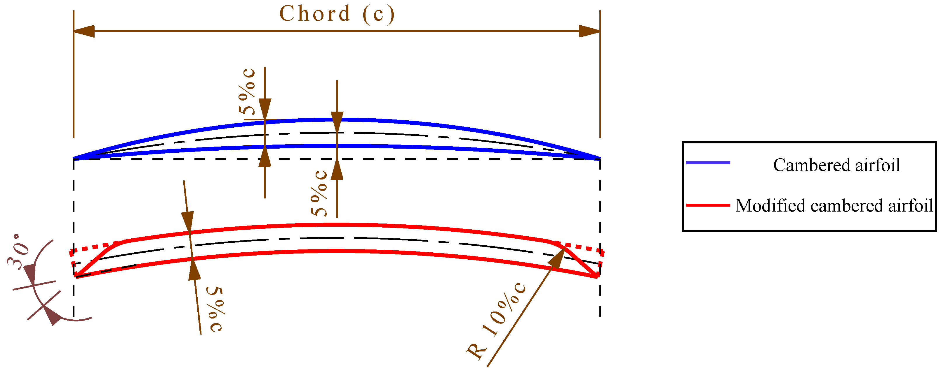
Moreover, as another advantage of thin cambered plates, they are found to be relatively insensitive to the turbulence level [35,37] and the surface roughness [36]. In order to satisfy the above-mentioned requirements, the airfoil is chosen to be a plate with a circular arc camber, maximum thickness and very sharp edges, as shown in Figure 1 with the blue color. The rotor was built from liquid photopolymer resin by 3D printing technology with a polyjet process and a resolution of 16 m. The first tests of the rotor in the wind tunnel revealed that rotor blades could not tolerate the incoming wind with high velocities and were slightly deformed during the measurements. Due to construction limitations, we therefore had to modify the airfoil geometry to a cambered plate with a constant thickness of and chamfered edges as shown in red color in Figure 1. This airfoil geometry is employed all along the rotor blade, except for the region very close to the blade root where the blade is thickened to improve the blade rigidity.
Based on the data reported in the above-mentioned studies on cambered airfoils in very low Reynolds numbers, the design angle of attack is chosen to be and the values of and at the design condition are estimated to be 0.75 and 13, respectively. Note that a rather conservative design angle of attack was chosen to avoid stall conditions, as similarly done in prior studies (e.g., [38]). It will be of interest to study the performance of the selected airfoil in future studies by means of wind-tunnel measurements or numerical simulations.
2.3. Design Tip-Speed Ratio
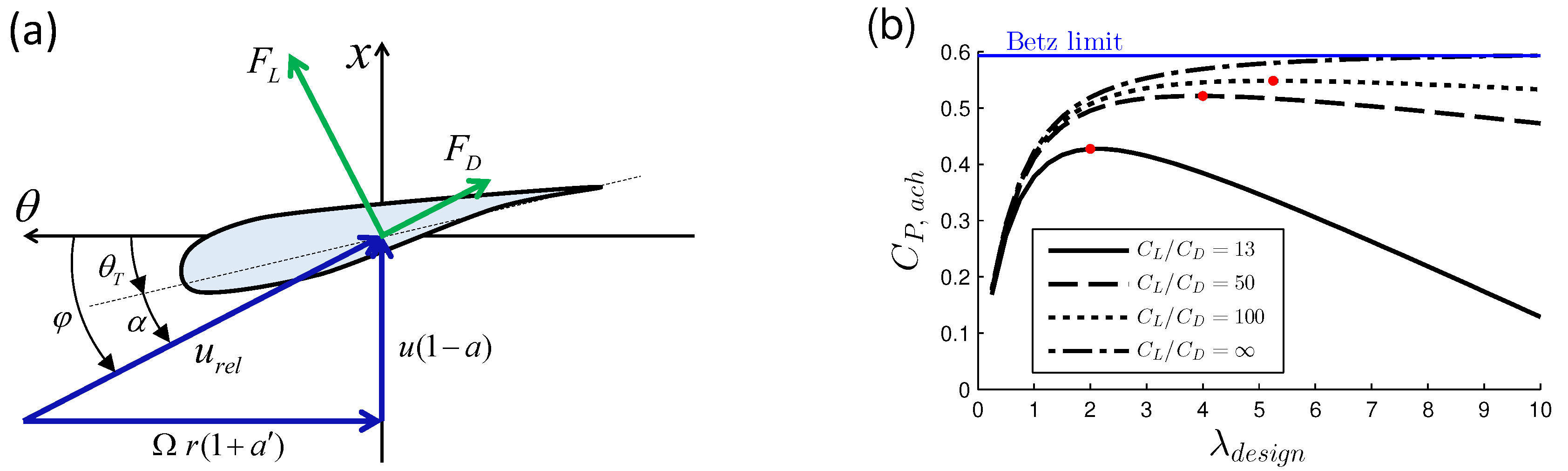
The tip-speed ratio is defined as , where R is the rotor radius and is the rotor rotational velocity. In order to select the design tip-speed ratio, one should consider different losses which prevent the turbine’s efficiency to reach the Betz limit. In addition to losses due to the wake rotation, drag losses can affect the power extracted by the turbine [33,39], especially for miniature turbines operating at very low Reynolds numbers. The former decreases with the increase of tip-speed ratio. In addition, the airfoil has a better performance at higher tip-speed ratios due to the higher operating Reynolds number. On the other hand, the effect of the drag force on the power reduction is more severe at higher design tip-speed ratios [40]. This can be readily explained by the schematic of the blade element shown in Figure 2a. As can be seen in the figure, the angle of the relative wind becomes smaller if the turbine is designed to rotate faster (i.e., higher design tip-speed ratios). This increases the projection of the drag force in the tangential direction (i.e., ), and decreases the one of the lift force (i.e., ). As a result, in contrast to wake-rotational losses, drag losses increase for higher design tip-speed ratios. There is therefore a specific design tip-speed ratio at which the achievable power is maximum for the turbine.
The effect of drag losses on the turbine performance can be seen quantitatively in Figure 2b. This figure shows the variation of the achievable power coefficient as a function of the design tip-speed ratio for different values of . In the following, we briefly explain how is computed for a given and . In general, the value of for a turbine can be calculated by [39]
where a and are the normal and angular induction factors, respectively, and is the local tip-speed ratio and equal to for a blade element located at the radial position r. Based on Glauert’s method, for each value of and , in Equation (3) has the optimal value (i.e., ) if [41]
From Figure 2a, can be expressed by
Solving the system of Equations (3)–(6) gives for a given and . The maximum value of for a given is indicated in Figure 2b with a red dot. As seen in the figure, the value of corresponding to the maximum achievable power increases with the increase of . As a result, for large-scale turbines is normally high given is quite high at high Reynolds numbers. For instance, the value of for the NREL 5MW rotor is [42]. Figure 2b, however, shows that the maximum achievable power for the miniature turbine (with estimated to be close to 13) occurs at , which is much lower than typical values of for large-scale turbines in the field. In order to have a design tip-speed ratio relatively closer to the one of large-scale turbines, while maintaining a high value of , we select the value of to be 4.5. It is worth mentioning that a higher value of (e.g., ) can be basically chosen for the miniature turbine. However, as shown in Figure 2b, this leads to a decrease in the value of achievable . In addition, the chord length and consequently the blade thickness decrease with the increase of . This imposes some difficulties regarding the built of the turbine with both enough accuracy and rigidity. Note that the effect of tip losses is neglected in the above discussion for the sake of simplicity. See Sørensen [41] and Sørensen et al. [24] for more information on tip losses and tip correction methods.
2.4. Optimum Chord and Twist Distributions
The optimum distributions of chord and twist were obtained based on Glauert’s optimum rotor [43]. See Sørensen [41] for a detailed discussion on the optimum rotor design. Figure 3 shows the chord and twist distributions of the rotor blade. In order to limit the size of the rotor hub and smooth the chord variation along the blade span, we had to modify the distribution of the chord especially close to the root as shown in the figure. We believe that this modification does not significantly affect the turbine performance as the modification affects mostly the region close to the root, which has only a small contribution to the total torque generation. Figure 4a shows a sketch of the new rotor. The three-dimensional sketch of the whole rotor can be found as an electronic Supplementary material from which detailed information on the rotor blade can be extracted. Moreover, the rotor can be readily employed by other researchers. To facilitate referring to this turbine rotor in future studies, we call it WiRE-01 rotor.
3. Wind Turbine Performance
3.1. Thrust Force
The turbine is placed in the WiRE wind tunnel under uniform inflow conditions. A highly sensitive multi-axis force sensor with the resolution of N is connected to the bottom of the turbine tower in order to measure the thrust force exerted on the turbine by the incoming wind. The free-stream velocity is measured with a Pitot tube. Both thrust and velocity measurements were performed for a period of 60 s with the sampling frequency of 1000 Hz. Figure 4b shows the variation of the thrust coefficient as a function of the tip-speed ratio . The figure shows that the value of for the miniature turbine reaches the value of 0.8, which is similar to the one of large-scale turbines in the field (e.g., for Vestas V80-2MW wind turbine [44]). As mentioned earlier, having realistic values of is very important as the overall strength of the wake largely depends on the value of . Figure 4b also shows that the value of slightly decreases for high tip-speed ratios, which has been also observed in prior wind tunnel studies (e.g., [10]). This behaviour is, however, in contrast with the common assumption that monotonically increases with the increase of the tip-speed ratio, usually observed for large-scale turbines [33]. In the following, we try to explain this discrepancy by studying the dependence of on for a single annulus.
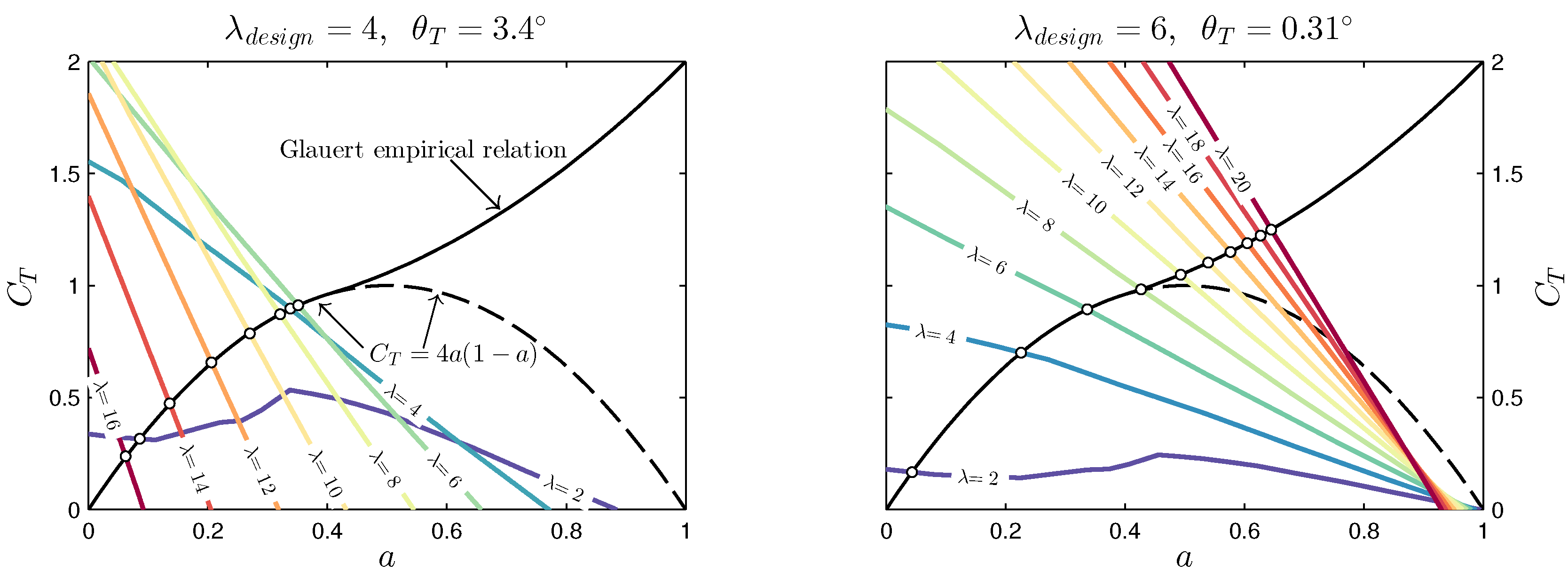
Let us consider an isolated single annulus with an arbitrary radius r containing B blade elements, where B is the number of blades (B = 3 here) with a local tip-speed ratio equal to . The airfoil geometry of the blade element is assumed to be NACA0012 operating at , which is in the range of for large-scale turbines. Blade-element momentum (BEM) analysis is performed to plot the variation of as a function of the normal induction factor a for the annulus in Figure 5. In Figure 5a, the design tip-speed ratio is 4 while it is 6 in Figure 5b. Based on the tabulated airfoil data [45], the value of and are selected as and , respectively, for both design tip-speed ratios. Colored lines show the value of for an annulus from the blade-element approach, whereas the black lines show the value of based on the momentum theory. Note that for (i.e., turbulent wake state), the Glauert empirical relation is plotted as the momentum theory is invalid in this region [39,46]. Based on the BEM theory, the intersection of each colored line with the solid black line shown by hollow circles in Figure 5 represents the operating condition of the blade element for the given tip-speed ratio [47]. As seen in the figure for , both values of and a increase monotonically with an increase of . Consequently, the blade element operates in turbulent wake state (i.e., ) at high tip-speed ratios. In contrast, for , both values of and a increase initially and then decrease with an increase of . In this case, the blade element ultimately operates in the propeller state (i.e., ) at very high tip-speed ratios. This explains why the variation of at high tip-speed ratios is different for the miniature turbine (Figure 4b) compared with large-scale turbines. Based on the above discussion, it is simply due to the selection of a lower design tip-speed ratio for the miniature turbine, and it is not caused by the difference in chord Reynolds number between the miniature turbine and its large-scale counterparts. Now, the question is why the variation of versus is so sensitive to . We try to answer this question by simplifying the governing equations for the considered annulus operating at high tip-speed ratios.
The value of for the annulus is given by [41]
where . Now, we simplify Equation (7) for . In this case, from Figure 2a, and one can therefore assume that and . Equation (7) can be then reduced to
The term in the above equation can be neglected with respect to unity as both and are small. Moreover, the angular induction factor is small at high tip-speed ratios, so from Figure 2a, . Equation (8) can be thus simplified to
For an ideal airfoil and small angles of attack, [48], where . Equation (9) can be therefore rewritten as
The above equation states that the value of has a linear relationship with a for high tip-speed ratios. The slope of this linear relationship is negative and its magnitude increases with an increase of . This is in agreement with the BEM predictions at high tip-speed ratios for both design tip-speed ratios shown in Figure 5. Furthermore, based on Equation (10), the x-intercept (i.e., ) of this linear relationship is a function of twist angle . For a low design tip-speed ratio, the twist angles is large, so the x-intercept rapidly decreases with an increase of . For a high design tip-speed ratio, in contrast, the twist angle can be either a small positive value or a negative one, so in both cases, the x-intercept does not largely decrease with an increase of . This is confirmed by Figure 5, showing that the x-intercept of the curves (colored lines) sharply decreases with increasing for (), while it experiences little change for (). The sharp decrease of the x-intercept of the colored lines in Figure 5 for leads to the reduction of the operating (intersecting point with the solid black line shown by hollow circles) for high tip-speed ratios. One can therefore conclude that the different variations of versus observed for different design tip-speed ratios are due to the difference in the value of the twist angle.
It is also important to note that a rotor contains multiple annuli at different radial positions. Thus even if a high value is chosen for the design tip speed ratio of the rotor, the local design tip-speed ratio for annuli close to the root of the rotor is much lower. This can explain why the central part of the rotor can operate as a propeller (i.e., ) at very high tip-speed ratios as experimentally observed by prior studies (e.g., [18,25]).
3.2. Power Extraction
3.2.1. Wind Turbine: Energy Conversion
As mentioned in Section 1, one of the crucial tasks in wind tunnel studies of wind turbines is to accurately determine the power extracted by the wind turbine (i.e., mechanical power ). The mechanical power is converted to electrical power in the generator as shown in Figure 6. All the mechanical input power is, however, not available for the conversion to electrical power, mainly due to friction losses. The converted power is denoted by in Figure 6 and it is equal to , where denotes power losses mainly due to the friction of the bearings and the friction between the moving parts of the machine and the air [49]. Moreover, as shown in the figure, is not entirely available at the machine’s electrical terminals. Some part of this converted power has to overcome electrical losses in the generator. Electrical losses are equal to , where R is the armature resistance plus the resistance of the brush contacts on the commutator [49]. Note that R is obviously different from the external resistance used to electrically load the generator.
In general, the converted power can be expressed in terms of , where is called electromagnetic torque [50] (also called armature torque [51]). Thus,
where and are the shaft torque (i.e., ) and the friction torque (i.e., ), respectively.
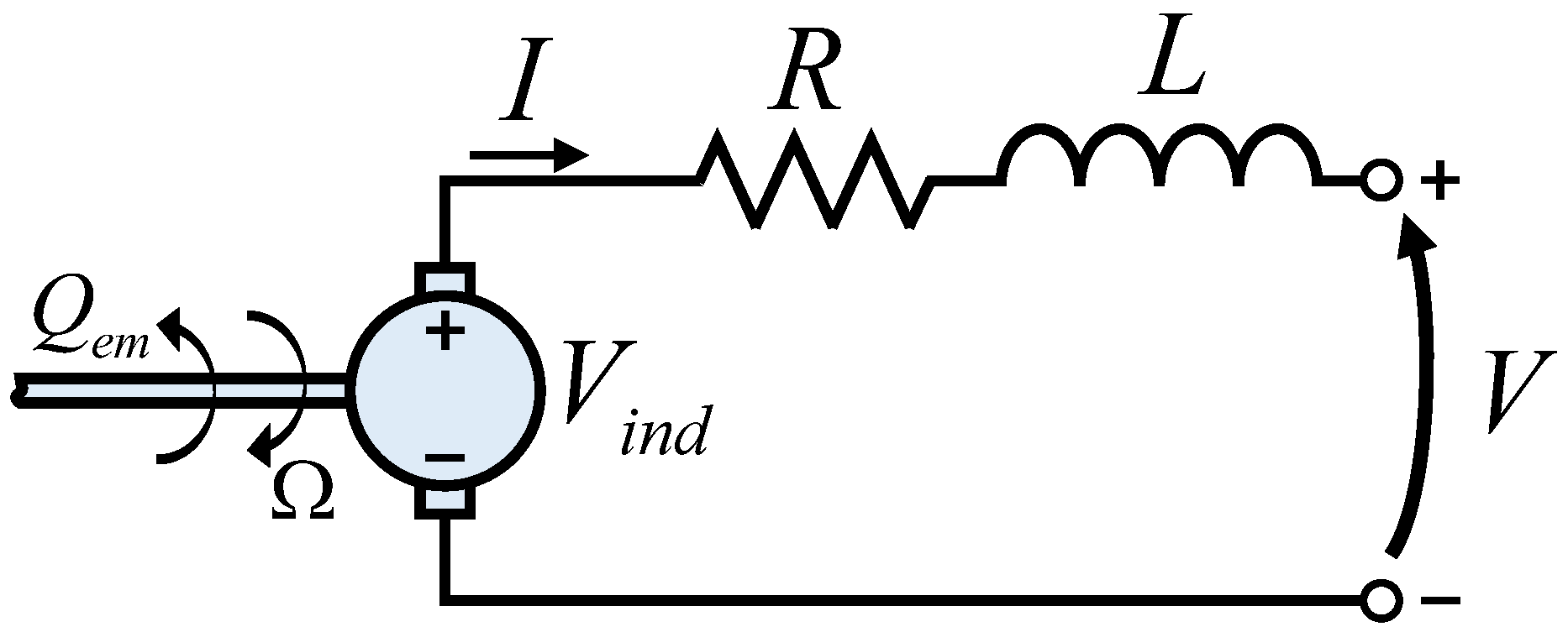
The generator used for small model wind turbines is usually a permanent-magnet DC (PMDC) machine. Figure 7 shows the equivalent electrical circuit of a PMDC machine in the generator mode. If a PMDC generator operates in steady-state conditions, the inductance L term in Figure 7 can be neglected [52,53]. Hence,
where is the induced voltage (i.e., induced electromotive force, EMF) due to the motion of the armature in the generator. Note that, from Equation (12), is always bigger than the terminal voltage V for a generator. Moreover, for PMDC machines in general, one can show that [53]
where K is called the EMF constant in Equation (13) and the torque constant in Equation (14). This constant is the same in the both equations if they are expressed in SI units. The value of K basically depends only on intrinsic characteristics of the PMDC machine (e.g., machine size, number of poles and magnetic field magnitude) and does not change with operating conditions [49].
Equation (14) can be used to find the electromagnetic torque . In order to estimate the value of the shaft torque , one has to therefore model the friction torque . In general, the friction torque varies with the rotational velocity . Different friction models (e.g., Stribeck friction) have been suggested in the literature [54,55,56,57]. A linear relationship between and the rotational velocity similar to the one used by Canudas et al. [54] is considered in this paper due to its simplicity. Hence,
where and are constants whose values can be estimated based on the DC-machine data provided by the manufacturer. Direct torque measurements will be employed in the following to see whether this method can acceptably predict the shaft torque .
3.2.2. Direct Measurement of Shaft Torque
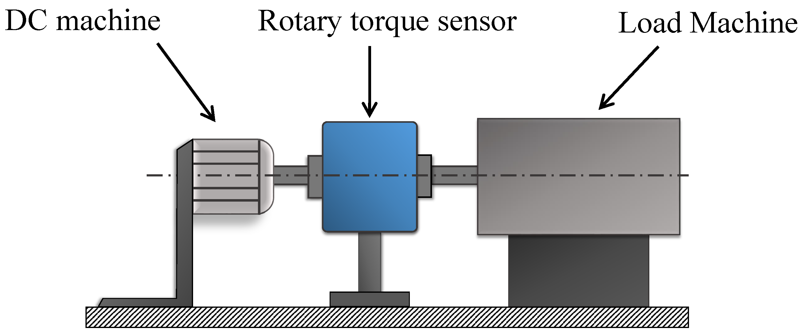
A high-precision rotary torque sensor from Scaime Inc, France. with an operating range of mNm and an accuracy equal to of full scale is used in the current study. In order to measure the shaft torque of the generator, the shaft of the rotary torque sensor is directly connected to the shaft of the generator. It is not practically possible to mount the torque sensor between the rotor and the DC generator in the wind tunnel. A separate setup is therefore built as shown in Figure 8. In this setup, a load machine which is basically a more powerful electrical motor simulates the incoming wind effect by rotating the shaft of the torque sensor and the DC machine. Both the load machine and the DC machine are connected to servo controllers so that their operating conditions are separately controlled and monitored. The rotational velocity of both of them are also measured by attached rotary encoders. Note that the use of a separate setup for torque measurements enables us to systematically study the effect of each variable (e.g., rotational velocity ) on the performance of the DC generator, keeping other variables (e.g., electrical current I) unchanged. This cannot be easily done if the torque sensor is directly connected to the miniature turbine in the wind tunnel.
In general, the operating condition of a miniature turbine can be uniquely described by the value of its rotational velocity and the generated electrical current. In this torque-sensor setup, the rotational velocity of the load machine and the generated electrical current of the DC machine are separately controlled. Therefore, any operating condition of the miniature turbine can be simulated by the torque-sensor setup. Note that the setup can be also used to measure the shaft torque of the DC machine in motor mode. To do so, we only need to reverse the direction of the energy conversion in the setup; i.e., the DC machine acts as a motor to rotate the load machine which acts as a generator in this case.
For the sake of completeness, we study the performance of three brushed DC machines with different sizes and power, all manufactured by Maxon company. All of them are suitable for being used in small-sized wind-turbine models. Table 1 shows their characteristics as provided by the manufacturer. A more powerful electrical machine with a nominal torque of 32 mNm is also used as the load machine.
Figure 9 shows the difference between the measured shaft torque and as a function of the rotational velocity for different electrical currents and DC machines in both generator and motor modes. If Equations (11) and (14) stated in Section 3.2.1 are valid for DC machines in real situations, should not depend on the electrical current I because, as mentioned earlier, it should be equal to the friction torque that varies only with the rotational velocity . The figure shows that, although the relationship between and slightly changes with the electrical current in some cases, the overall agreement is acceptable and one can assume that . Note that the small disagreement specially observed for DC-machine II might be due to the fairly inaccurate value of the torque constant K provided by the manufacturer.
The conclusion drawn above is in contrast with what was suggested by Kang and Meneveau [27] in their pioneering study. They compared the manufacturer-provided data with measured quantities and reported a significant deviation. Specifically, they compared the value of with the measured , and showed that there is a big difference between them. In addition, they showed that V is not linearly proportional to . Firstly, note that should be compared with , which is clearly bigger than due to the electrical losses. Secondly, as stated in Equation (13), is supposed to be linearly proportional to , not V. In fact, even from their own data, the shaft torque is found to be linearly proportional to the electrical current, and the value of the slope for this linear relationship is very similar to the manufacturer-provided value of the torque constant K (Equation (4) in Kang and Meneveau [27]). This in turn confirms the fact that .
Figure 9 also shows that the value of is bigger than in the generator mode while it is smaller than in the motor mode. This is expected as the energy is converted from the electrical form to the mechanical one in motors, contrary to generators. Furthermore, it can be seen that the friction torque increases with the increase of rotational speed , as expected. The figure also shows that a linear relationship similar to Equation (15) can acceptably approximate the variation of with , even though a polynomial fit matches better. One possible explanation for this non-linear behavior is that core losses are neglected in this study compared to friction losses. See Chapman [49] for more information.
The data shown in Figure 9 can be used to find the values of and in Equation (15). We, however, wonder how well theses values can be estimated based on the data of the DC machines provided by the manufacturer. This could be of great interest particularly for those who cannot perform direct torque measurements and therefore can only use the manufacturer-provided data. To do so, one can use the DC-machine data at nominal and no-load operating conditions presented in Table 1. Note that manufacturer-provided data are usually for DC machines in motor mode. By using these data, hence, we implicitly assume that the magnitude of the friction torque is similar for both modes, which is supported by the data of Figure 9. At nominal conditions, friction torque is equal to for a DC motor, where and are the electrical current and the shaft torque at nominal conditions, respectively. At no-load conditions, is equal to zero for a DC motor and thereby , where is the electrical current at no-load conditions. The predictions of the based on the data of Table 1 are shown by black solid lines in Figure 9. Clearly, they are not in good agreement with the measured data, especially for DC machines I and III. However, they might be still useful for making a rough estimation about the magnitude of the friction torque. This will be further discussed in the following.
3.2.3. Power Coefficient of the Miniature Turbine
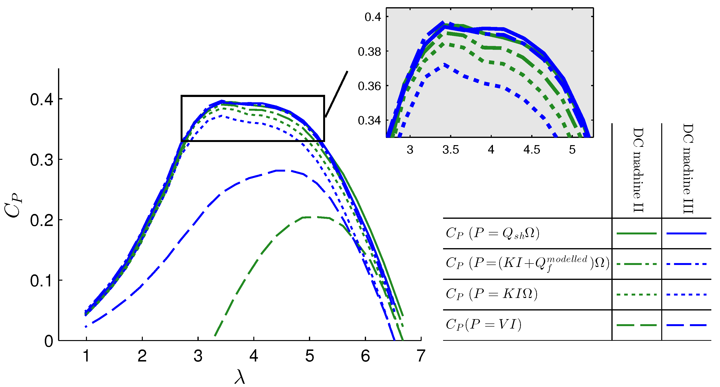
Figure 10 shows the variation of the power coefficient of the miniature turbine as a function of the tip-speed ratio at the free-stream velocity of 8 ms. In order to change the tip-speed ratio, a servo controller (ESCON 36/2 DC from Maxon, Switzerland) is used to change the electrical loads on the DC generator, thereby controlling the turbine rotational velocity. To see the effect of the DC generator on the wind-turbine performance, the data are shown for the rotor connected to both DC generators II and III under the same incoming flow conditions. For each DC generator, the value of the power P is calculated based on: (i) the measured shaft torque multiplied by ; (ii) the electromagnetic torque multiplied by ; (iii) the electromagnetic torque plus the friction torque multiplied by , where is estimated based on the data provided by the manufacturer as discussed in Section 3.2.2; and finally (iv) the terminal voltage V times the electrical current I. As shown in the figure, the value of based on the measured mechanical input power () is very similar for both cases. This is expected as the mechanical power does not depend on generator characteristics. The figure also shows that the values of based on the converted power (i.e., ) are smaller than the ones based on the mechanical power, and they are different for the two DC machines. This can be explained by the fact that and the value of friction losses (i.e., ) depend on generator characteristics. It is also interesting to note that the difference between and is smaller for lower tip-speed ratios. At lower tip-speed ratios, the turbine rotates slower so the friction torque is smaller. Moreover, the value of the electromagnetic torque is generally quite high for low tip-speed ratios, so the friction torque becomes less important.
By modeling the friction torque (Equation (15)) and adding it to the converted power, the figure shows that one can have a rather acceptable estimation of the mechanical input power. This approximation method is more promising if the shaft torque is not much smaller than the nominal value because, in this case, the friction torque is likely to be negligible compared to the electromagnetic torque. The DC machine should not, however, work beyond the nominal operating range as the linear proportionality between the electromagnetic torque and the electrical current does not necessarily hold anymore, and working in these conditions can also permanently damage the machine [58]. It is also important to remind that DC-machine characteristics change with temperature, so the manufacturer-provided data are not likely to be reliable at high temperatures [58].
Figure 10 also shows the value of based on the generated electrical power for both DC generators. As seen in the figure and also shown by Kang and Meneveau [27], the generated power is much smaller than the extracted one due to mechanical and electrical losses. More importantly, the figure shows that the use of electrical power can lead to misleading information on wind turbine characteristics. For instance, it significantly overestimates the value of the optimal tip-speed ratio , at which the extracted power is maximum. The reason is that electrical losses in the generator (i.e., ) rapidly increase with the increase of the electrical current I. The value of therefore becomes very small for lower tip-speed ratios (i.e., higher electrical currents). This is why the maximum generated power in Figure 10 occurs at tip-speed ratios higher than the optimal one.
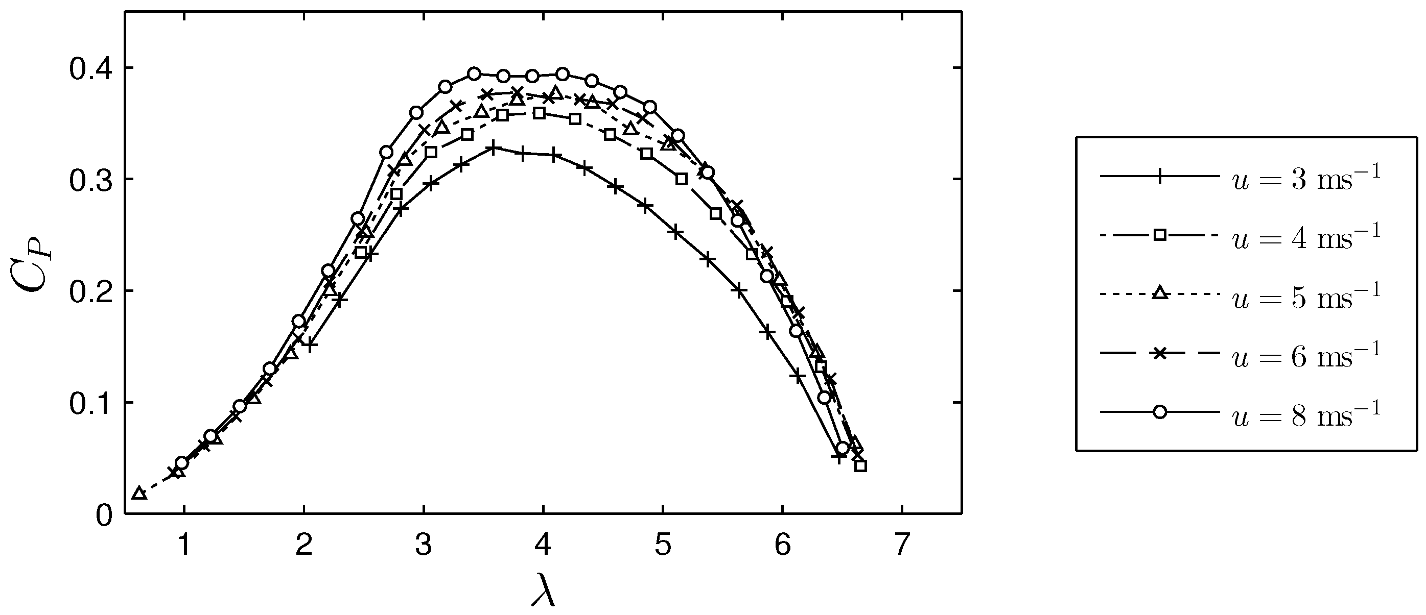
The variation of the power coefficient (based on measured ) with the tip-speed ratio is shown in Figure 11 for different incoming free-stream velocities. As seen in the figure, the value of increases with the increase of the incoming flow velocity, which is due to the better performance of the rotor blades at higher Reynolds numbers. This means that the value of for the miniature turbine varies with both tip-speed ratio and wind speed, which is in agreement with prior studies (e.g., [25]). The dependence of on the wind speed is expected to be less for utility-scale turbines as the airfoil performance does not significantly change with wind speed at high Reynolds numbers. The value of for the miniature turbine can be as high as 0.4 as shown in the figure, which is quite remarkable for a miniature wind turbine with cm. The optimal tip-speed ratio varies slightly with the change of the incoming velocity but overall the best performance occurs at which is smaller than the design tip-speed ratio (). The difference is due to the use of likely inaccurate airfoil design information.
An uncertainty analysis is also provided in Appendix A to estimate the uncertainty of measurements for the miniature turbine. It is found that the value of the relative standard uncertainty for is about and at the optimal tip-speed ratio for equal to 5 m/s and 8 m/s, respectively.
4. Summary
A new three-bladed horizontal-axis miniature wind turbine with a diameter of 15 cm, suitable for wind tunnel studies of wind turbine wakes and wind farm flows, is designed and fully characterized in this study. The main motivation for the design of a new miniature turbine is to achieve higher and more realistic (similar to those of field-scale turbines) values of and , compared with previously used miniature wind turbines. A new blade profile, a thick plate with a circular arc camber and sharp leading edge, is employed for the new miniature turbine. The turbine designed based on Glauert’s optimum rotor with a design tip-speed ratio equal to 4.5 is built with 3D-printing technology.
Force measurements are performed in the wind tunnel to calculate the thrust coefficient of the miniature turbine. The magnitude of of the miniature turbine is found to be around at the optimal tip-speed ratio, which is similar to the one of large-scale turbines. Moreover, it is found that the value of slightly decreases at high tip-speed ratios for the miniature turbine, contrary to the one of large-scale turbines. A simple theoretical analysis is employed to show that the variation of with tip-speed ratio can be different at high tip-speed ratios depending on the value of the blade twist angle.
For the sake of accurate measurement of the turbine extracted power, a new setup is developed to directly measure the torque of the rotor shaft. A high-precision rotary torque sensor with an operating range of mNm is directly connected to the DC generator, and a load machine simulates the incoming wind effect by rotating the shaft of the torque sensor and the DC generator. The measurements show that the value of power coefficient can reach to around , which is considerable for a miniature turbine with this small size. Particular attention is also focused on the conversion of mechanical energy into electrical one in the generator. To this end, the performance of three different DC generators is systematically studied for various operating conditions. It is found that the use of the manufacturer-provided data for the tested generators can yield a fairly acceptable estimation of the turbine extracted power.
Flow dynamics and wake characteristics (e.g., meandering motion) of the new miniature wind turbine under boundary-layer inflow conditions are presented in Part II of this study [59].
Supplementary Materials
The following is available online at www.mdpi.com/1996-1073/10/7/908/s1, File S1: Three-dimensional sketch of WiRE-01 rotor.
Acknowledgments
This research was supported by the Swiss National Science Foundation (grant 200021_172538, and grant 206021_144976), the Swiss Federal Office of Energy (grant SI/501337-01), and the Swiss Innovation and Technology Committee (CTI) within the context of the Swiss Competence Center for Energy Research “FURIES: Future Swiss Electrical Infrastructure”. The first author was also partially supported by the EuroTech Greentech Initiative Wind Energy. The authors would also like to thank Messrs. S. Eghbali, T. Curran and A. Jungo for their efforts in preparation of the torque-sensor setup. Special thanks also go to M. Bozorg and H. Sekhavatmanesh for their insightful comments on the electrical parts of the paper.
Author Contributions
This study was done as a part of Majid Bastankhah’s doctoral studies supervised by Fernando Porté-Agel.
Conflicts of Interest
The authors declare no conflict of interest.
Appendix A
This appendix contains an uncertainty analysis of power coefficient measurements for the miniature wind turbine. The incoming free-stream velocity is obtained from Pitot-tube measurements, and thus it is equal to , where is the dynamic pressure measured with the Pitot tube. The value of stated in Equation (1) can be therefore written as
The overall uncertainty of denoted by can be calculated from
where , , , , and are the uncertainties of Q, , Q, , and A, respectively. Note that in Equation (A2), uncertainties of measured variables are assumed to be independent from each other, and thus the correlation terms are neglected. See Coleman and Steele [60] for more information. The uncertainty for each variable is due to both random and bias errors. The former is, however, relatively negligible provided the variables are averaged over a long enough time period. In the following, the uncertainty of each variable due to the bias error will be discussed:
- Uncertainty of Q: Based on the data provided by the manufacturer, the uncertainty of the measured torque Q is estimated to be mNm.
- Uncertainty of : The rotational velocity is measured with a rotary digital encoder with 128 counts per turn so its uncertainty can be assumed to be negligible with respect to those for other variables.
- Uncertainty of : The air density is estimated based on the ideal gas law; i.e., , where is the atmospheric pressure, is the specific gas constant of air and is the air temperature measured with a thermometer. The value of can be therefore obtained fromwhere and are the uncertainties of and , respectively. The former is estimated to be of based on the meteorological data in relation to the static pressure distribution over Switzerland, and the latter is 0.5 based on the manufacturer data.
- Uncertainty of : The uncertainty of is due to the systematic error associated with the Pitot tube and the error of the pressure transducer . Based on the data provided by the manufacturers, the former is of the measured value and the latter is approximately Pa. The overall value of is then equal to .
- Uncertainty of A: It is equal to , where is the uncertainty of R (equal to 16 m for the employed 3D-printer system).
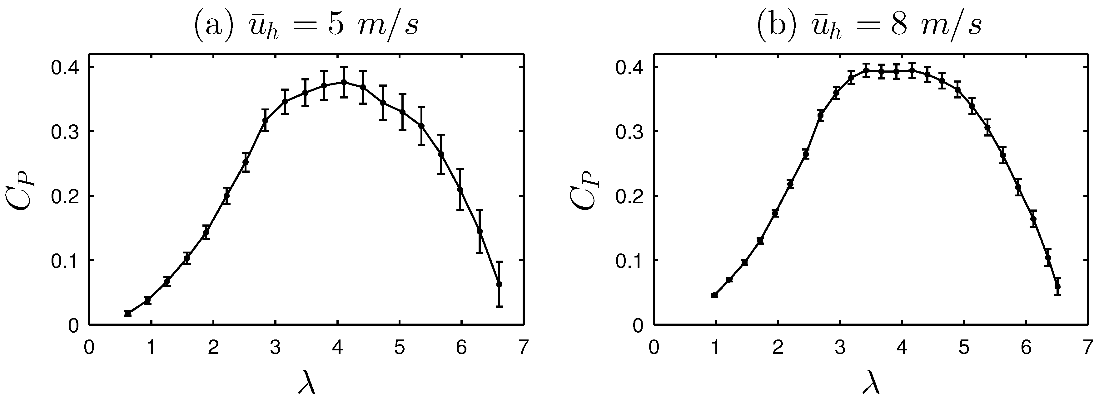
Now, the overall uncertainty of can be calculated. In general, among the uncertainty terms of the measured variables in Equation (A2), those related to the torque Q (i.e., first term on the right-hand side) and the dynamic pressure (i.e., fourth term on the right-hand side) are found to be the dominant ones. It is also worth mentioning that, as the confidence level of the uncertainties provided by manufacturers is not usually reported, we assume that they are all standard uncertainties (i.e., with the confidence level of ) which is a rather conservative assumption. Figure A1 shows the variation of with for two different incoming velocities, and the values of the standard uncertainty are also shown with error bars in the figure. As seen in both Figure A1a,b, the value of the uncertainty decreases with the decrease of the tip-speed ratio. This is due to the fact that all the terms on the right-hand side of Equation (A2) except for the neglected second term are proportional to the rotational velocity , so the overall uncertainty reduces at lower tip-speed ratios. Moreover, the figure shows that the measurement uncertainty decreases by increasing the incoming velocity. At the optimal tip-speed ratio, the value of the relative standard uncertainty for is about and for equal to 5 m/s and 8 m/s, respectively.
Figure A1.
Variation of the power coefficient of the miniature turbine with the tip-speed ratio for two different incoming velocities: (a) m/s and (b) m/s. Error bars indicate values of the standard uncertainty.
Figure A1.
Variation of the power coefficient of the miniature turbine with the tip-speed ratio for two different incoming velocities: (a) m/s and (b) m/s. Error bars indicate values of the standard uncertainty.

References
- Vermeer, L.; Sørensen, J.; Crespo, A. Wind turbine wake aerodynamics. Prog. Aerosp. Sci. 2003, 39, 467–510. [Google Scholar] [CrossRef]
- Medici, D.; Alfredsson, P. Measurement on a wind turbine wake: 3D effects and bluff body vortex shedding. Wind Energy 2006, 9, 219–236. [Google Scholar] [CrossRef]
- Cal, R.B.; Lebrón, J.; Castillo, L.; Kang, H.S.; Meneveau, C. Experimental study of the horizontally averaged flow structure in a model wind-turbine array boundary layer. J. Renew. Sustain. Energy 2010, 2, 013106. [Google Scholar] [CrossRef]
- Chamorro, L.P.; Porté-Agel, F. A wind-tunnel investigation of wind-turbine wakes: Boundary-layer turbulence effects. Bound.-Layer Meteorol. 2009, 132, 129–149. [Google Scholar] [CrossRef]
- Chamorro, L.P.; Porté-Agel, F. Effects of thermal stability and incoming boundary-layer flow characteristics on wind-turbine wakes: A wind-tunnel study. Bound.-Layer Meterol. 2010, 136, 515–533. [Google Scholar] [CrossRef]
- Chamorro, L.P.; Porté-Agel, F. Turbulent flow inside and above a wind farm: A wind-tunnel study. Energies 2011, 4, 1916–1936. [Google Scholar] [CrossRef]
- España, G.; Aubrun, S.; Loyer, S.; Devinant, P. Spatial study of the wake meandering using modelled wind turbines in a wind tunnel. Wind Energy 2011, 14, 923–937. [Google Scholar] [CrossRef]
- España, G.; Aubrun, S.; Loyer, S.; Devinant, P. Wind tunnel study of the wake meandering downstream of a modelled wind turbine as an effect of large scale turbulent eddies. J. Wind Eng. Ind. Aerodyn. 2012, 101, 24–33. [Google Scholar] [CrossRef]
- Markfort, C.; Zhang, W.; Porté-Agel, F. Turbulent flow and scalar transport through and over aligned and staggered wind farms. J. Turbul. 2012, 13, N33. [Google Scholar] [CrossRef]
- Yang, Z.; Sarkar, P.; Hu, H. Visualization of the tip vortices in a wind turbine wake. J. Vis. 2012, 15, 39–44. [Google Scholar] [CrossRef]
- Zhang, W.; Markfort, C.D.; Porté-Agel, F. Near-wake flow structure downwind of a wind turbine in a turbulent boundary layer. Exp. Fluids 2012, 52, 1219–1235. [Google Scholar] [CrossRef]
- Zhang, W.; Markfort, C.D.; Porté-Agel, F. Wind-turbine wakes in a convective boundary layer: A wind-tunnel study. Bound.-Layer Meteorol. 2013, 146, 161–179. [Google Scholar] [CrossRef]
- Iungo, G.V.; Viola, F.; Camarri, S.; Porté-Agel, F.; Gallaire, F. Linear stability analysis of wind turbine wakes performed on wind tunnel measurements. J. Fluid Mech. 2013, 737, 499–526. [Google Scholar] [CrossRef]
- Viola, F.; Iungo, G.V.; Camarri, S.; Porté-Agel, F.; Gallaire, F. Prediction of the hub vortex instability in a wind turbine wake: Stability analysis with eddy-viscosity models calibrated on wind tunnel data. J. Fluid Mech. 2014, 750, R1. [Google Scholar] [CrossRef]
- Hancock, P.; Pascheke, F. Wind-tunnel simulation of the wake of a large wind turbine in a stable boundary layer: Part 2, the wake flow. Bound.-Layer Meteorol. 2014, 151, 23–37. [Google Scholar] [CrossRef]
- Hancock, P.; Zhang, S. A wind-tunnel simulation of the wake of a large wind turbine in a weakly unstable boundary layer. Bound.-Layer Meteorol. 2015, 156, 395–413. [Google Scholar] [CrossRef]
- Tobin, N.; Hamed, A.M.; Chamorro, L.P. An experimental study on the effects of winglets on the wake and performance of a model wind turbine. Energies 2015, 8, 11955–11972. [Google Scholar] [CrossRef]
- Bastankhah, M.; Porté-Agel, F. A wind-tunnel investigation of wind-turbine wakes in yawed conditions. J. Phys. Conf. Ser. 2015, 625, 012014. [Google Scholar] [CrossRef]
- Bastankhah, M.; Porté-Agel, F. Experimental and theoretical study of wind turbine wakes in yawed conditions. J. Fluid Mech. 2016, 806, 506–541. [Google Scholar] [CrossRef]
- Howland, M.F.; Bossuyt, J.; Martinez-Tossas, L.A.; Meyers, J.; Meneveau, C. Wake structure in actuator disk models of wind turbines in yaw under uniform inflow conditions. J. Renew. Sustain. Energy 2016, 8, 043301. [Google Scholar] [CrossRef]
- Bastankhah, M.; Porté-Agel, F. Wind tunnel study of the wind turbine interaction with a boundary-layer flow: Upwind region, turbine performance, and wake region. Phys. Fluids 2017, 29, 065105. [Google Scholar] [CrossRef]
- Bastankhah, M.; Porté-Agel, F. A new analytical model for wind-turbine wakes. Renew. Energy 2014, 70, 116–123. [Google Scholar] [CrossRef]
- Odemark, Y.; Fransson, J.H. The stability and development of tip and root vortices behind a model wind turbine. Exp. Fluids 2013, 54, 1–16. [Google Scholar] [CrossRef]
- Sørensen, J.N.; Okulov, V.; Mikkelsen, R.F.; Naumov, I.; Litvinov, I. Comparison of classical methods for blade design and the influence of tip correction on rotor performance. J. Phys. Conf. Ser. 2016, 753, 022020. [Google Scholar] [CrossRef]
- Krogstad, P.; Adaramola, M.S. Performance and near wake measurements of a model horizontal axis wind turbine. Wind Energy 2012, 15, 743–756. [Google Scholar] [CrossRef]
- Bottasso, C.L.; Campagnolo, F.; Petrović, V. Wind tunnel testing of scaled wind turbine models: Beyond aerodynamics. Wind Eng. Ind. Aerodyn. 2014, 127, 11–28. [Google Scholar] [CrossRef]
- Kang, H.; Meneveau, C. Direct mechanical torque sensor for model wind turbines. Meas. Sci. Technol. 2010, 21, 105206. [Google Scholar] [CrossRef]
- Howard, K.; Hu, J.; Chamorro, L.; Guala, M. Characterizing the response of a wind turbine model under complex inflow conditions. Wind Energy 2015, 18, 729–743. [Google Scholar] [CrossRef]
- Ozbay, A.; Tian, W.; Yang, Z.; Hu, H. Interference of Wind Turbines with Different Yaw Angles of the Upstream Wind Turbine. In Proceedings of the 42nd AIAA Fluid Dynamics Conference and Exhibit, New Orleans, LA, USA, 25–28 June 2012; p. 2719. [Google Scholar]
- Stein, V.P.; Kaltenbach, H.J. Wind-tunnel modelling of the tip-speed ratio influence on the wake evolution. J. Phys. Conf. Ser. 2016, 753, 032061. [Google Scholar] [CrossRef]
- Qing’an, L.; Murata, J.; Endo, M.; Maeda, T.; Kamada, Y. Experimental and numerical investigation of the effect of turbulent inflow on a Horizontal Axis Wind Turbine (Part I: Power performance). Energy 2016, 113, 713–722. [Google Scholar]
- Garratt, J.R. Review: The atmospheric boundary layer. Earth-Sci. Rev. 1994, 37, 89–134. [Google Scholar] [CrossRef]
- Burton, T.; Sharpe, D.; Jenkins, N.; Bossanyi, E. Wind Energy Handbook, 1st ed.; Wiley: Hoboken, NJ, USA, 1995; p. 617. [Google Scholar]
- Sunada, S.; Sakaguchi, A.; Kawachi, K. Airfoil section characteristics at a low Reynolds number. J. Fluids Eng. 1997, 119, 129–135. [Google Scholar] [CrossRef]
- Laitone, E. Wind tunnel tests of wings at Reynolds numbers below 70 000. Exp. Fluids 1997, 23, 405–409. [Google Scholar] [CrossRef]
- Sunada, S.; Yasuda, T.; Yasuda, K.; Kawachi, K. Comparison of wing characteristics at an ultralow Reynolds number. J. Aircr. 2002, 39, 331–338. [Google Scholar] [CrossRef]
- Pelletier, A.; Mueller, T.J. Low reynolds number aerodynamics of low-aspect-ratio, thin/flat/cambered-plate wings. J. Aircr. 2000, 37, 825–832. [Google Scholar] [CrossRef]
- Sherry, M.; Nemes, A.; Jacono, D.L.; Blackburn, H.M.; Sheridan, J. The interaction of helical tip and root vortices in a wind turbine wake. Phys. Fluids (1994-present) 2013, 25, 117102. [Google Scholar] [CrossRef]
- Manwell, J.F.; McGowan, J.G.; Rogers, A.L. Wind Energy Explained: Theory, Design and Application; John Wiley & Sons: Hoboken, NJ, USA, 2010. [Google Scholar]
- Wilson, R.E.; Lissaman, P.B.; Walker, S.N. Aerodynamic Performance of Wind Turbines; Final Report, Technical Report; Oregon State University, Department of Mechanical Engineering: Corvallis, OR, USA, 1976. [Google Scholar]
- Sørensen, J.N. General Momentum Theory for Horizontal Axis Wind Turbines; Springer: Cham, Switzerland, 2015. [Google Scholar]
- Jonkman, J.; Butterfield, S.; Musial, W.; Scott, G. Definition of a 5-MW Reference Wind Turbine for Offshore System Development; Technical Report No. NREL/TP-500-38060; National Renewable Energy Laborary: Golden, CO, USA, 2009.
- Glauert, H. Airplane propellers. In Aerodynamic Theory; Springer: Berlin/Heidelberg, Germany, 1935; pp. 169–360. [Google Scholar]
- Hansen, K.S.; Barthelmie, R.J.; Jensen, L.E.; Sommer, A. The impact of turbulence intensity and atmospheric stability on power deficits due to wind turbine wakes at Horns Rev wind farm. Wind Energy 2012, 15, 183–196. [Google Scholar] [CrossRef]
- Sheldahl, R.E.; Klimas, P.C. Aerodynamic Characteristics of Seven Symmetrical Airfoil Sections through 180-Degree Angle of Attack for Use in Aerodynamic Analysis of Vertical Axis Wind Turbines; Technical Report; Sandia National Laboratories: Albuquerque, NM, USA, 1981.
- Spera, D.A. Wind Turbine Technology; ASME Press: New York, NY, USA, 1994. [Google Scholar]
- Wilson, R.E.; Lissaman, P.B. Applied Aerodynamics of Wind Power Machines; Technical Report; Oregon State University: Corvallis, OR, USA, 1974. [Google Scholar]
- Abbott, I.H.; Von Doenhoff, A.E. Theory of Wing Sections, Including a Summary of Airfoil Data; Courier Corporation: North Chelmsford, MA, USA, 1959. [Google Scholar]
- Chapman, S. Electric Machinery Fundamentals; Tata McGraw-Hill Education: New York, NY, USA, 2005. [Google Scholar]
- Sen, P.C. Principles of Electric Machines and Power Electronics; John Wiley & Sons: Hoboken, NJ, USA, 2007. [Google Scholar]
- Theraja, B.; Theraja, A.K. A Text Book of Electrical Technology; S Chand & Co. Ltd.: New Delhi, India, 2006. [Google Scholar]
- Sharma, S. Basics of Electrical Engineering; IK International Pvt Ltd.: New Delhi, India, 2007. [Google Scholar]
- Hughes, A. Electric Motors and Drives: Fundamentals, Types and Applications; Newnes: Boston, MA, USA, 2013. [Google Scholar]
- Canudas, C.; Astrom, K.; Braun, K. Adaptive friction compensation in DC-motor drives. IEEE J. Robot. Autom. 1987, 3, 681–685. [Google Scholar] [CrossRef]
- Armstrong, B. Friction: Experimental determination, modeling and compensation. In Proceedings of the 1988 IEEE International Conference on Robotics and Automation, Philadelphia, PA, USA, 24–29 April 1988; pp. 1422–1427. [Google Scholar]
- Olsson, H.; Åström, K.J.; De Wit, C.C.; Gäfvert, M.; Lischinsky, P. Friction models and friction compensation. Eur. J. Control 1998, 4, 176–195. [Google Scholar] [CrossRef]
- Tjahjowidodo, T.; Al-Bender, F.; Van Brussel, H.; Symens, W. Friction characterization and compensation in electro-mechanical systems. J. Sound Vib. 2007, 308, 632–646. [Google Scholar] [CrossRef]
- Krishnan, R. Permanent Magnet Synchronous and Brushless DC Motor Drives; CRC Press: Boca Raton, FL, USA, 2009. [Google Scholar]
- Bastankhah, M.; Porté-Agel, F. A new miniature wind turbine for wind tunnel experiments. Part II: Wake structure and Flow dynamics. Energies 2017, in press. [Google Scholar]
- Coleman, H.W.; Steele, W.G. Experimentation, Validation, and Uncertainty Analysis for Engineers; John Wiley & Sons: Hoboken, NJ, USA, 2009. [Google Scholar]
Figure 1.
Airfoil geometry: the cambered plate with very thin edges (blue color), and the cambered plate with constant thickness modified due to construction limits (red color).
Figure 1.
Airfoil geometry: the cambered plate with very thin edges (blue color), and the cambered plate with constant thickness modified due to construction limits (red color).

Figure 2.
(a) The velocity triangle for a rotor blade element; (b) Achievable power coefficient as a function of the design tip-speed ratio for different values of . The maximum achievable power for each is shown with a red dot.
Figure 2.
(a) The velocity triangle for a rotor blade element; (b) Achievable power coefficient as a function of the design tip-speed ratio for different values of . The maximum achievable power for each is shown with a red dot.

Figure 3.
Twist and chord distributions for the blade of the miniature turbine shown by blue circles. The ones suggested by the Glauert design method are shown with black lines.
Figure 3.
Twist and chord distributions for the blade of the miniature turbine shown by blue circles. The ones suggested by the Glauert design method are shown with black lines.
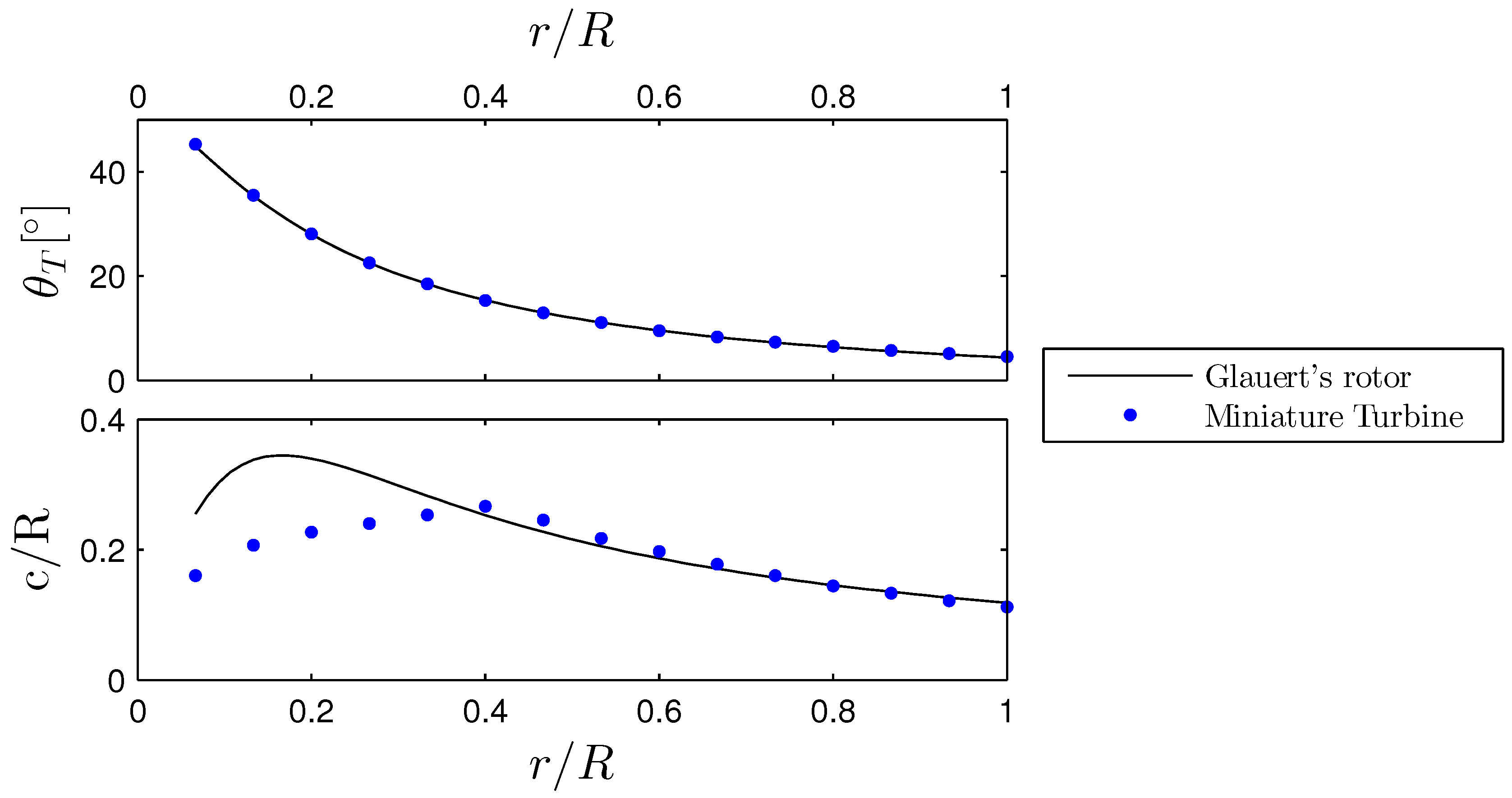
Figure 4.
(a) Sketch of the new designed turbine rotor; (b) Variation of the thrust coefficient of the miniature turbine with the tip-speed ratio at m/s.
Figure 4.
(a) Sketch of the new designed turbine rotor; (b) Variation of the thrust coefficient of the miniature turbine with the tip-speed ratio at m/s.
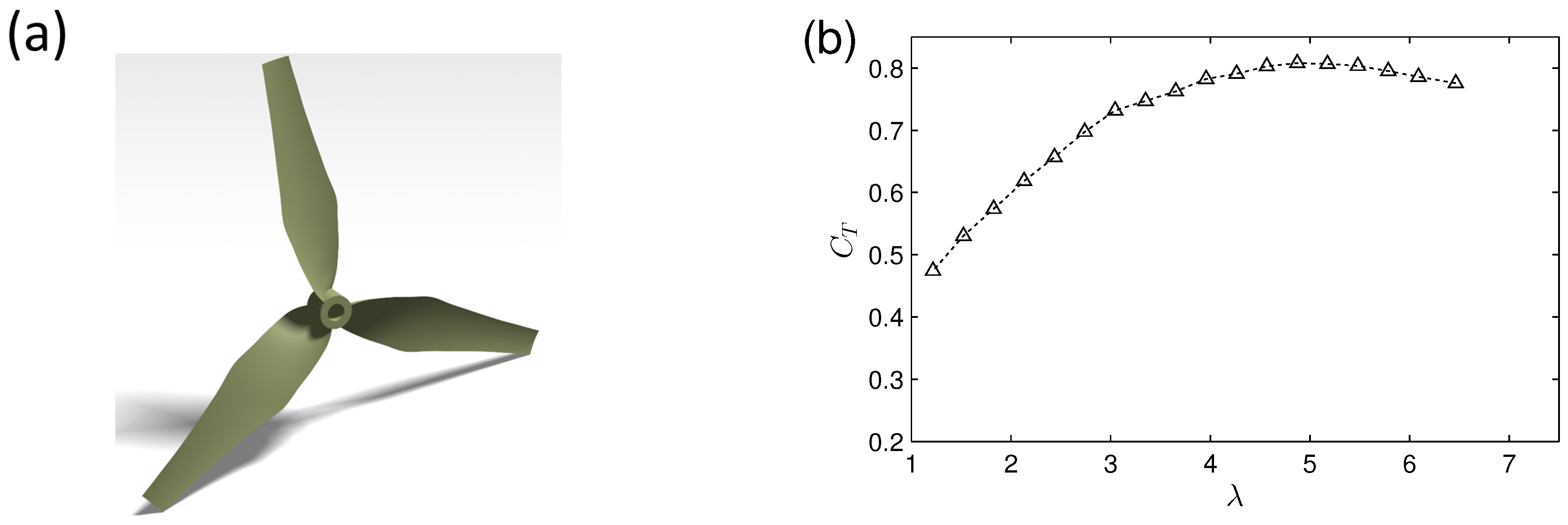
Figure 5.
Variation of the thrust coefficient with the normal induction factor a for an annulus at two different design tip-speed ratios ( and 6). The airfoil profile is NACA0012, operating at . The black lines represent the relationship based on the momentum approach, while the colored lines show it from the blade-element approach. For each tip-speed ratio, the operating condition is indicated by hollow white circles.

Figure 6.
Energy conversion in a miniature wind turbine.
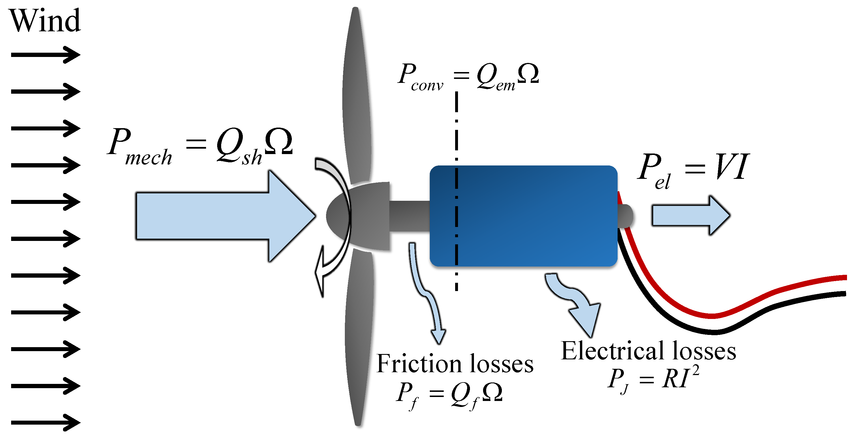
Figure 7.
Equivalent electrical circuit of a permanent magnet DC generator.

Figure 8.
Schematic of the setup for direct measurements of the shaft torque of DC generators.

Figure 9.
Measured values of () versus the rotational velocity for different electrical currents and DC machines in both motor and generation modes. The black lines show the prediction of the friction torque based on Equation (15) and using the manufacturer-provided data.
Figure 9.
Measured values of () versus the rotational velocity for different electrical currents and DC machines in both motor and generation modes. The black lines show the prediction of the friction torque based on Equation (15) and using the manufacturer-provided data.
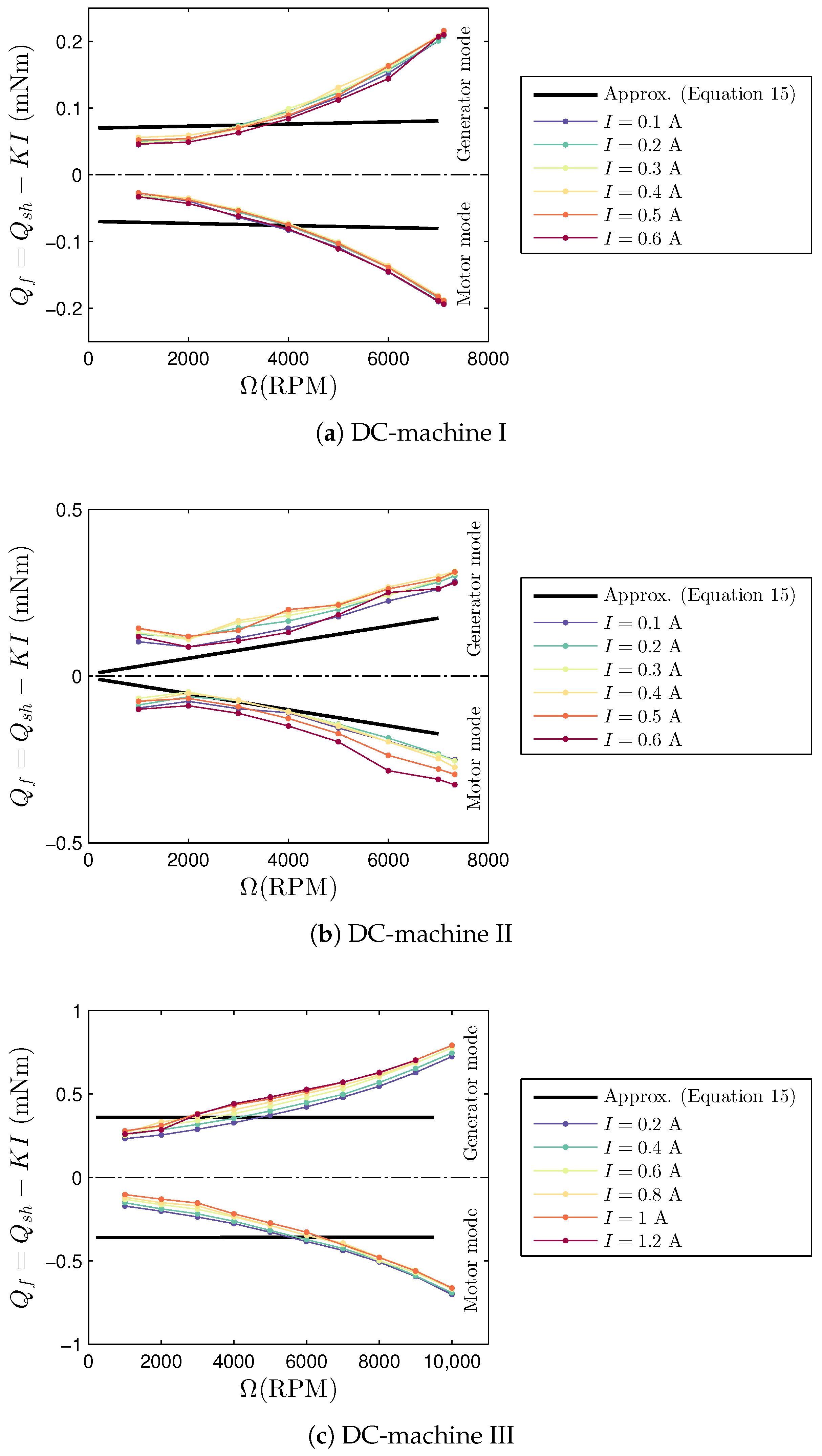
Figure 10.
Variation of the power coefficient with the tip-speed ratio for the miniature turbine with two different DC machines under the same inflow conditions. For each DC machine, the turbine power is calculated with different methods. The free-stream incoming velocity is equal to 8 ms.
Figure 10.
Variation of the power coefficient with the tip-speed ratio for the miniature turbine with two different DC machines under the same inflow conditions. For each DC machine, the turbine power is calculated with different methods. The free-stream incoming velocity is equal to 8 ms.

Figure 11.
Variation of the power coefficient of the miniature turbine with the tip-speed ratio at different free-stream incoming velocities.
Figure 11.
Variation of the power coefficient of the miniature turbine with the tip-speed ratio at different free-stream incoming velocities.

Table 1.
Manufacturer-provided data of the DC machines studied in this paper.
| DC-Machine I | DC-Machine II | DC-Machine III | ||
|---|---|---|---|---|
| DCX10L | DCX14L | DCX16L | ||
| Outer diameter (mm) | 10 | 14 | 16 | |
| Nominal voltage (V) | 4.5 | 12 | 9 | |
| Nominal speed (rpm) | 7110 | 7330 | 11,100 | |
| Nominal torque (mNm) | 2.2 | 6.86 | 11.9 | |
| Nominal current (A) | 0.648 | 0.646 | 1.88 | |
| No load speed (rpm) | 12000 | 10,300 | 13,100 | |
| No load current (mA) | 25.2 | 23.2 | 54.8 | |
| Torque constant (mNm/A) | K | 3.52 | 10.9 | 6.52 |
© 2017 by the authors. Licensee MDPI, Basel, Switzerland. This article is an open access article distributed under the terms and conditions of the Creative Commons Attribution (CC BY) license (http://creativecommons.org/licenses/by/4.0/).
Share and Cite
MDPI and ACS Style
Bastankhah, M.; Porté-Agel, F. A New Miniature Wind Turbine for Wind Tunnel Experiments. Part I: Design and Performance. Energies 2017, 10, 908. https://doi.org/10.3390/en10070908
AMA Style
Bastankhah M, Porté-Agel F. A New Miniature Wind Turbine for Wind Tunnel Experiments. Part I: Design and Performance. Energies. 2017; 10(7):908. https://doi.org/10.3390/en10070908
Chicago/Turabian StyleBastankhah, Majid, and Fernando Porté-Agel. 2017. "A New Miniature Wind Turbine for Wind Tunnel Experiments. Part I: Design and Performance" Energies 10, no. 7: 908. https://doi.org/10.3390/en10070908
Note that from the first issue of 2016, this journal uses article numbers instead of page numbers. See further details here.