A New Hybrid Wind Power Forecaster Using the Beveridge-Nelson Decomposition Method and a Relevance Vector Machine Optimized by the Ant Lion Optimizer

Abstract

As one of the most promising kinds of the renewable energy power, wind power has developed rapidly in recent years. However, wind power has the characteristics of intermittency and volatility, so its penetration into electric power systems brings challenges for their safe and stable operation, therefore making accurate wind power forecasting increasingly important, which is also a challenging task. In this paper, a new hybrid wind power forecasting method, named the BND-ALO-RVM forecaster, is proposed. It combines the Beveridge-Nelson decomposition method (BND), relevance vector machine (RVM) and ant lion optimizer (ALO). Considering the nonlinear and non-stationary characteristics of wind power data, the wind power time series were firstly decomposed into deterministic, cyclical and stochastic components using BND. Then, these three decomposed components were respectively forecasted using RVM. Meanwhile, to improve the forecasting performance, the kernel width parameter of RVM was optimally determined by ALO, a new Nature-inspired meta-heuristic algorithm. Finally, the wind power forecasting result was obtained by multiplying the forecasting results of those three components. The proposed BND-ALO-RVM wind power forecaster was tested with real-world hourly wind power data from the Xinjiang Uygur autonomous region in China. To verify the effectiveness and feasibility of the proposed forecaster, it was compared with single RVM without time series decomposition and parameter optimization, RVM with time series decomposition based on BND (BND-RVM), RVM with parameter optimization (ALO-RVM), and Generalized Regression Neural Network with data decomposition based on Wavelet Transform (WT-GRNN) using three forecasting performance criteria, namely MAE (Mean Absolute Error), MAPE (Mean Absolute Percentage Error) and RMSE (Root Mean Square Error). The results indicate the proposed BND-ALO-RVM wind power forecaster has the best forecasting performance of all the tested options, which confirms its validity.

1. Introduction

Facing the unfavorable situation of fossil energy resource depletion and environmental deterioration, people are increasingly focusing on the exploitation and utilization of renewable energy resources, such as wind power and solar photovoltaic power [1]. Nowadays, wind power has become one of the fastest growing and most promising renewable energy power sources, and the share of wind power generation in the total electricity output has been increasing yearly [2,3]. According to the data released by the Global Wind Energy Council, by the end of 2016, the installed wind power capacity around the world reached 486.7 GW. The cumulative installed wind power capacity in China amounts to 168.7 GW, which accounts for 34.7% of the world total.

Wind power is environmentally friendly. However, wind power output has the characteristics of stochastic fluctuation, intermittency and uncertainty [4]. When a wind generator is connected to the power grid, it will impose new requirements and challenges on electric power systems, such as efficient scheduling of power resources and continuing guarantee of smooth power system operation [5]. With the increase of wind power penetration, it is necessary to increase operation costs to deal with the electric energy unbalance issues due to the stochastic fluctuation of wind power [6]. Meanwhile, to coordinate with wind generators, thermal power generating units have no choice but to frequently adjust their power output, which will reduce the operational efficiency and increase running costs [7]. Accurate wind power forecasting is an effective and important way to alleviate the abovementioned adverse effects.

In past years, many researchers have developed models and methods for wind power/speed forecasting, which have made great achievements [8,9]. Currently, there are mainly two kinds of forecasting techniques related to wind power/speed, which are physical-based forecasting techniques and statistical-based forecasting techniques. Physical forecasting techniques represent a traditional forecasting approach, which needs detailed physical descriptions related to the on-site conditions of wind farms, such as the wind farm layout, wind turbines, and atmospheric conditions [10]. The main representatives are Prediktor developed by the Risoe National Laboratory in Denmark [11], Previento developed by University of Oldenburg in Germany [12], and eWind developed by AWS True Wind Inc. (New York, NY, USA) [13]. In the past few years, statistical forecasting techniques, which conduct wind power/speed forecasting based on historical power/speed data and other meteorological data have been developed greatly. This kind of forecasting technique includes two kinds of approaches, namely conventional statistical approaches and emerging artificial intelligent approaches. Among conventional statistical approaches, the auto-regressive moving average (ARMA) model [14,15] and auto-regressive integrated moving average (ARIMA) model [16] have been widely used to forecast wind speed and wind power. The conventional statistical approaches hold the assumption that wind power and wind speed have linear relationships with their influencing factors. However, in fact, the relationships between wind power/speed and their influencing factors are non-linear. Therefore, the conventional statistical approaches fall short of obtaining high forecasting accuracy and satisfactory forecasting results. The other statistical forecasting techniques, namely the emerging artificial intelligence approaches, do not assume a linear relationship between wind power/speed and their influencing factors can effectively cover the abovementioned shortcomings of conventional statistical approaches. Currently, there are several emerging artificial intelligence approaches which have been employed to forecast wind power and wind speed, such as artificial neural networks [17,18], support vector machine [19], and extreme learning machine [20,21].

When emerging artificial intelligence approaches are employed to forecast wind power/speed, there are several parameters that must be set first, such as neuron number of artificial neural networks and kernel parameters of support vector machines. This is very difficult for practitioners. To tackle this issue, an intelligent optimization algorithm is usually introduced to determine the optimal parameters of emerging artificial intelligence approaches. Ren, et al. [22] applied particle swam optimization (PSO) to automatically determine the parameters of a back propagation neural network (BPNN) for short-term wind speed forecasting. Amjady, et al. [23] used enhanced particle swarm optimization to optimize a modified neural network for wind power prediction. Jursa and Rohrig [24] employed PSO and differential evolution (DE) to optimize artificial neural networks for short-term wind power forecasting. Liu, et al. [25] used a genetic algorithm to select the optimal parameters of support vector machines for short-term wind speed forecasting. Salcedo-Sanz, et al. [26] used a coral reefs optimization algorithm to optimize an extreme learning machine for wind speed prediction.

Generally speaking, wind power time series have both nonlinear and nonstationary characteristics, so the decomposition of wind power time series is often needed to improve wind power forecasting accuracy [27]. Currently, there are mainly two kinds of wind power time series decomposition methods, which are the wavelet transform (WT) [28,29] and empirical mode decomposition (EMD) [30,31]. The Beveridge-Nelson decomposition (BND) method, proposed by researchers Stephen Beveridge and Charles Nelson in 1981, is a kind of non-stationary time series decomposition technique [32], which has been widely applied in economic fields, such as business cycle analysis [33], GNP and stock prices [34], and regional income fluctuations [35]. As an effective time series decomposition method, it is very regretful to find that the BND has not been used for wind power time series. To fill this gap, in this paper the BND technique is employed to decompose wind power time series, which is a new application.

In this paper, relevance vector machine (RVM), a kind of sparse and supervised learning probabilistic method, is also used for wind power forecasting. RVM has some merits compared with other machine learning methods, such as better adaptability, a need for fewer sample data, sparsity, and simplified parameter setting [36]. Nowadays, RVM is employed in many practical issues, such as silent speech classification [37], battery health monitoring [38], canal flow prediction [39], daily potential evapotranspiration forecast [40], and system fault diagnosis [41]. However, the RVM technique has rarely been used for wind power forecasting. To improve RVM-based forecasting performance of wind power, a new Nature-inspired meta-heuristic algorithm, named the ant lion optimizer (ALO) [42] is also employed in this paper to automatically determine the optimal parameters of RVM. Therefore, a new hybrid BND-ALO-RVM method for wind power forecasting is proposed in this paper. To verify the effectiveness and applicability of this proposed method, real-world hourly wind power data from the Xinjiang Uygur autonomous region in China is selected as our empirical analysis example, and the forecasting results are compared with other forecasting methods, including single RVM, BND-RVM, ALO-RVM, and WT-GRNN. The main contributions of this paper are as follows:

(1)

A new hybrid BND-ALO-RVM method for wind power forecasting is proposed, which combines Beveridge-Nelson decomposition (BND), relevance vector machine (RVM) and ant lion optimizer (ALO). Empirical results indicate that the proposed method can improve wind power forecasting accuracy and shows superiority over other compared methods. The proposed method in this paper can be a promising alternative forecasting technique for wind power, which enriches the current wind power forecasting method toolbox.

(2)

The Beveridge-Nelson decomposition (BND) method, which has been frequently and widely used for economic issues, is employed in energy issues for the first time. In this paper, the wind power time series are decomposed into three components, namely the deterministic, cyclical and stochastic component. Empirical results show the wind power forecasting accuracy can be improved after decomposing wind power time series by using BND, which indicates BND is an effective method for wind power time series decomposition. It can be said that this paper expands the application domains of the BND method, and enriches the data decomposition library for wind power time series.

(3)

Relevance vector machine (RVM) technique is employed to forecast the different decomposed components of wind power time series. To improve the forecasting performance of RVM, a new Nature-inspired meta-heuristic algorithm, namely the ant lion optimizer (ALO), is used to optimally determine the kernel width parameter of RVM model. Forecasting results reveal the ALO is effective, which can determine the optimal kernel width parameter of RVM and improve the RVM-based wind power forecasting accuracy. In our previous study [43], has was verified that the ALO can improve GM (1,1)-based power load forecasting accuracy. Therefore, ALO, as a new intelligent optimization algorithm, can be promising with a good development foreground. This paper makes a new attempt to use ALO for parameter optimization of RVM, which also enlarges the application scope of the ALO algorithm.

The reminder of this paper is organized as follow: Section 2 gives a brief introduction of the basic methods and algorithms used, including the Beveridge-Nelson decomposition (BND) method, relevance vector machine (RVM), and ant lion optimizer (ALO); the proposed hybrid BND-ALO-RVM forecaster for wind power is described in Section 3; Section 4 conducts an empirical analysis, and the forecasting performance of the proposed method is compared with other methods. The main conclusions are drawn in Section 5.

2. Brief Introduction of the Beveridge-Nelson Decomposition Method, Relevance Vector Machine and Ant Lion Optimizer

2.1. Beveridge-Nelson Decomposition Method (BND)

In 1981, two researchers Stephen Beveridge and Charles Nelson proposed a new general procedure for non-stationary time series decomposition, named the Beveridge-Nelson decomposition (BND) method [32]. The BND method decomposes the stationary first-order difference of original time series with first-order co-integration characteristics into permanent components and transitory (cyclical) components [44]. The permanent component is a random walk process with drift, which includes deterministic component and stochastic component. The deterministic component can be estimated using ARIMA technique, and the transitory (cyclical) component is a stationary process with a zero average value.

The first step of the BND method is to determine whether the first-order difference of a non-stationary wind power time series is stationary or not [45]. If yes, the detailed steps of wind power time series decomposition by using BND method are as follows:

The wind power time series are represented as WP. According to the Wold theorem, under the the condition of first-order stationarity, the natural logarithm of the wind power time series at time t (denoted as lnWP_t) satisfies:

$$\Delta \ln W{P}_t=\mu +{\epsilon }_t+{\displaystyle \sum _{i=1}^{\infty }{\lambda }_i{\epsilon }_{t-i}}$$

(1)

where WP_t is the wind power at time t; μ is the long-run mean value of ΔlnWP_t; ${\epsilon }_t~i.i.d.N\left(0,{\sigma }^2\right)$ (i.i.d. represents independently and identically distribute); ${\lambda }_i$ is the coefficient; and $\Delta \ln W{P}_t=\ln W{P}_t-\ln W{P}_{t-1}$.

Taking the expectation on both sides of Equation (1), we can obtain:

$$E\left(\Delta \ln W{P}_t\right)=E\left(\mu \right)+E\left({\epsilon }_t\right)+E\left({\displaystyle \sum _{i=1}^{\infty }{\lambda }_i{\epsilon }_{t-i}}\right)=E\left(\mu \right)$$

(2)

where $E(•)$ represents the expected computation on variables.

According to the Beveridge-Nelson decomposition theorem, the deterministic component (represented as $D_t$) of the wind power time series can be decomposed as:

$$D_t=\ln W{P}_0+\mu t$$

(3)

where D_t represents the deterministic component of the wind power time series at time t; and lnWP₀ is the natural logarithm value of the initial wind power data.

According to Morley [44], the time series can be forecasted by using first-order difference AR(1) model, namely:

$$\left(\Delta \ln W{P}_t-\mu \right)=\varphi \left(\Delta \ln W{P}_{t-1}-\mu \right)+{\epsilon }_t$$

(4)

where $\left|\varphi \right|<1$, and ${\epsilon }_t~i.i.d.N\left(0,{\sigma }^2\right)$.

According to the Wold theorem, the expected value of minimum mean squared error (MMSE) of first-order difference ΔlnWP_t at next j period under the assumption of normality is:

$$E_t\left[\left(\Delta \ln W{P}_{t+j}-\mu \right)\right]={\varphi }^j\left(\Delta \ln W{P}_t-\mu \right)$$

(5)

The BN trend of wind power time series, denoted as T_t, is defined as the MMSE forecast of time series long-term level, namely:

$$T_t=\underset{j\to \infty }{\lim }{E}_t\left[\left(\ln W{P}_{t+j}-j\mu \right)\right]=\ln W{P}_t+\underset{j\to \infty }{\lim }{E}_t\left[\left(\Delta \ln W{P}_{t+j}-\mu \right)\right]$$

(6)

Thus, substituting Equation (5) into Equation (6), the BN trend of lnWP_t for the case AR (1) can be obtained as:

$$T_t=\ln WP+\frac{\varphi }{1-\varphi }\left(\Delta \ln W{P}_t-\mu \right)$$

(7)

Meanwhile, the cyclical component $C_t$ of wind power time series can be calculated by:

$$C_t=-\frac{\varphi }{1-\varphi }\left(\Delta \ln W{P}_t-\mu \right)$$

(8)

Finally, the stochastic component $T_t$ of wind power time series can be computed as:

$$T_t=\ln WP+\frac{\varphi }{1-\varphi }\left(\Delta \ln W{P}_t-\mu \right)-\left(\ln W{P}_0+\mu t\right)$$

(9)

2.2. Relevance Vector Machine (RVM)

Relevance vector machine (RVM), proposed by Tipping, is a kind of sparse and supervised learning probabilistic method [46]. Compared with traditional supervised learning algorithms, RVM under a Bayesian framework has a better non-linear mapping capability, which can be used in the case of a small number of samples and can also obtain a good generalization performance.

Given a training sample set ${\left\{p_i,v_i\right\}}_{i=1}^N$, $p_i$ is a two-dimensional input vector, and $v_i$ is a one-dimensional target value. The RVM model can be formulated as:

$$y\left(p,w\right)={\displaystyle \sum _{i=1}^N{w}_{i}K\left(p,p_i\right)}+w_0$$

(10)

where N is the number of training sample; $w_i$ is the weight; and $K\left(p,p_i\right)$ is a kernel function.

There are several kinds of kernel functions, and the Gaussian kernel function is usually employed, namely:

$$K\left(p,p_i\right)=\exp \left(\frac{-\Vert p-p_i\Vert }{2{\sigma }^2}\right)$$

(11)

where $\sigma$ is the width of kernel function.

Suppose that the noise ${\epsilon }_i$ obeys normal distribution with mean of 0 and variance ${\sigma }^2$. Then:

$$v_i=y\left(p_i,w\right)+{\epsilon }_i$$

(12)

Since $v_i$ is independent and identically distributed, the likelihood function of the training sample is:

$$P\left(v|w,{\sigma }^2\right)=\frac{1}{\sqrt{2\pi }\sigma }\exp \left(\frac{-{\Vert v-\mathsf{\Phi }w\Vert }^2}{2{\sigma }^2}\right)$$

(13)

where $v={\left(v_1,v_2,\cdots ,v_N\right)}^T$; $w={\left(w_0,w_1,\cdots ,w_n\right)}^T$; ${\mathsf{\Phi }}_{N\times \left(N+1\right)}={\left[\varphi \left(p_1\right),\varphi \left(p_2\right),\cdots ,\varphi \left(p_N\right)\right]}^T$; and $\varphi \left(p_i\right)=\left[1,K\left(p_i,p_1\right),\cdots ,K\left(p_i,p_N\right)\right]$.

To avoid the issues of too many relevance vectors, over-fitting and poor generalization capability, the weight $w$ should obey normal distribution, namely:

$$P\left(w|\alpha \right)={\displaystyle \prod _{i=0}^N\frac{{\alpha }_i}{\sqrt{2\pi }}\exp \left(-\frac{{\alpha }_i{w}_i^2}{2}\right)}$$

(14)

According to the Bayesian criterion, it can be inferred that the a posteriori distributions of w and t are both normal distributions, namely:

$$P\left(v|\alpha ,{\sigma }^2\right)=\frac{1}{\sqrt{{\left(2\pi \right)}^N\left({\sigma }^{2}I+\mathsf{\Phi }{A}^{-1}{\mathsf{\Phi }}^T\right)}}\exp \left(-\frac{v^{T}v}{2\left({\sigma }^{2}I+\mathsf{\Phi }{A}^{-1}{\mathsf{\Phi }}^T\right)}\right)$$

(15)

$$P\left(w|v,\alpha ,{\sigma }^2\right)=\frac{P\left(v|w,{\sigma }^2\right)P\left(w|\alpha \right)}{P\left(v|\alpha ,{\sigma }^2\right)}=\frac{i}{\sqrt{{\left(2\pi \right)}^{N+1}{\displaystyle {\sum }^1}}}\exp \left\{-\frac{{\left(w-\mu \right)}^T\left(w-\mu \right)}{2{\displaystyle {\sum }^1}}\right\}$$

(16)

where $\mu ={\sigma }^{-2}\left({\sigma }^{2}I+\Phi A^{-1}{\mathsf{\Phi }}^T\right){\mathsf{\Phi }}^{T}v$; ${\displaystyle {\sum }^1}={\left({\sigma }^{-2}{\mathsf{\Phi }}^T\mathsf{\Phi }+A\right)}^{-1}$; $A=diag\left({\alpha }_0,{\alpha }_1,\cdots ,{\alpha }_N\right)$.

To maximize the hyper-parameter likelihood distribution $P\left(v|\alpha ,{\sigma }^2\right)$, the optimal values of ${\alpha }^{best}$ and ${\sigma }_{best}^2$ can be obtain according to the following iterations, namely:

$${\alpha }_i^{best}=\frac{1-{\alpha }_i{N}_{ii}}{{\mu }_i^2}$$

(17)

$${\sigma }_{best}^2=\frac{{\Vert v-\mathsf{\Phi }\mu \Vert }^2}{N-{\displaystyle \sum _{i=0}^N\left(1-{\alpha }_i{N}_{ii}\right)}}$$

(18)

where ${\alpha }_i^{best}$ is the ith value of optimal parameter ${\alpha }^{best}$; ${\mu }_i$ is the ith posterior mean value of $\mu$; and $N_{ii}$ is the ith diagonal element of posterior variance matrix.

When the new input data $p^{*}$ is given, the corresponding probability distribution of forecasting output can be obtained as:

$$P\left(v^{*}|v,{\alpha }^{best},{\sigma }_{best}^2\right)={\displaystyle \int P\left(v^{*}|w,{\sigma }_{best}^2\right)P\left(w|v,{\alpha }^{best},{\sigma }_{best}^2\right)}dw$$

(19)

The forecasting variance is:

$${\sigma }_{*}^2={\sigma }_{best}^2+\varphi {\left(p^{*}\right)}^T{\displaystyle {\sum }^1}\varphi \left(p^{*}\right)$$

(20)

The mean value of the forecasting output is:

$$y^{*}={\mu }^T\varphi \left(p^{*}\right)$$

(21)

During the parameter estimation process, most ${\alpha }_i$ will tend to $\infty$, and then the corresponding $w_i$ will equal 0. This means that many terms of the kernel matrix will not participate in the forecasting process, and this is why RVM can achieve sparsity [36]. Compared with the support vector machine (SVM) technique, there is only one parameter which needs to be set for RVM, namely the kernel width parameter $\sigma$ [36].

2.3. Ant Lion Optimizer (ALO)

In 2015, Mirjalili proposed a new Nature-inspired meta-heuristic algorithm, namely the ant lion optimizer (ALO) [42]. The ALO was put forward by the inspiration of intelligence behavior of ant lions hunting for ants. The detailed steps of the ALO algorithm are as follows:

Step 1: Set initial parameters.

When ALO is used, the initial values of five parameters need to be set, which are the number of ants and ant lions Agents_no; maximum iteration number Max_iteration; variables number dim; lower bound $lb=\left[l{b}_1,l{b}_2,\cdots \right]$ and upper bound $ub=\left[u{b}_1,u{b}_2,\cdots \right]$ of variables.

Step 2: Initialize the positions of ants and antlions.

The positions of ants and antlions need to be initialized, which can be represented by Equations (22) and (23).

$$M_{Ant}=\left[\begin{array}{cccc}{A}_{11}& A_{12}& \cdots & A_{1d}\\ A_{21}& A_{22}& \cdots & A_{2d}\\ ⋮& ⋮& ⋮& ⋮\\ A_{n1}& A_{n2}& \cdots & A_{nd}\end{array}\right]$$

(22)

$$M_{Antlion}=\left[\begin{array}{cccc}A{L}_{11}& A{L}_{12}& \cdots & A{L}_{1d}\\ A{L}_{21}& A{L}_{22}& \cdots & A{L}_{2d}\\ ⋮& ⋮& ⋮& ⋮\\ A{L}_{n1}& A{L}_{n2}& \cdots & A{L}_{nd}\end{array}\right]$$

(23)

where $M_{Ant}$ represents each ant position; $A_{ij}$ represents the j-th parameter’s value of the i-th ant; $M_{Antlion}$ represents each antlion position; $A{L}_{ij}$ represents the j-th parameter’s value of the i-th antlion; $i=1,2,\cdots ,n$, $j=1,2,\cdots ,d$.

The positions of ants and antlions are generated at random. Therefore, the entry of position matrix of ant and antlion can be obtained according to Equation (24):

$$A_{\ast j}orA{L}_{\ast j}=rand\times \left(u{b}_j-l{b}_j\right)+l{b}_j$$

(24)

where $A_{\ast j}$ and $A{L}_{\ast j}$ are the j-th column values of position matrix; rand represents the generated random number with uniform distribution in the interval [0, 1]; $l{b}_j$ and $u{b}_j$ respectively, represent the lower and upper boundary of the j-th variable.

Step 3: Select initial elite.

The elite refers to the best antlion obtained in the iteration process. The best antlion can be determined according to fitness function, and the antlion with the maximal fitness value is elite, which is also called as the fittest antlion. In ALO, the fitness function of antlion is represented by $f[\ast ]$, and matrix $M_{OAL}$ is used to store fitness values of antlions, namely:

$$M_{OAL}=\left\{\begin{array}{c}f\left[\left(\begin{array}{cccc}A{L}_{11}& A{L}_{12}& \cdots & A{L}_{1d}\end{array}\right)\right]\\ f\left[\left(\begin{array}{cccc}A{L}_{21}& A{L}_{22}& \cdots & A{L}_{2d}\end{array}\right)\right]\\ ⋮\\ f\left[\left(\begin{array}{cccc}A{L}_{n1}& A{L}_{n2}& \cdots & A{L}_{nd}\end{array}\right)\right]\end{array}\right\}$$

(25)

where $M_{OAL}$ is the fitness matrix of antlions.

According to Equation (25), the fitness values of antlions can be calculated, and then the initial elite can be selected.

Step 4: Start iteration.

In ALO, the ant position is influenced by both the antlion and the selected elite. The ants randomly walk around the selected elite and antlions are selected by a roulette wheel algorithm. According to this rule, the i-th ant position at the t-th iteration can be obtained by:

$$An{t}_i^t=\frac{R_E^t+R_A^t}{2}$$

(26)

where $An{t}_i^t$ is the i-th ant position at the t-th iteration, $R_E^t$ represents the random walk around the selected elite at the t-th iteration, and $R_A^t$ represents the random walk around the antlion selected by the roulette wheel algorithm.

Random walk is an important strategy for modelling the positions and movements of ants and antlions in the ALO algorithm. For a detailed interpretation related to random walk in ALO readers can refer to [42,43].

In the iteration process, the ants update their positions according to Equation (26). In order to keep the random walk inside the search space, the ant position needs to be normalized at each iteration as follows:

$${\tilde{X}}_j^t=\frac{\left(X_j^t-a_j\right)\times \left(d_j^t-c_j^t\right)}{\left(b_j-a_j\right)}+c_j^t$$

(27)

where ${\tilde{X}}_j^t$ represents the normalized value of the j-th variable at the t-th iteration; $a_j$ and $b_j$ respectively represent the minimum and maximum of random walk of the j-th variable; $c_j^t$ and $d_j^t$ are the minimum and maximum of random walk of the j-th variable at t-th iteration, respectively.

In the ALO algorithm, the random walk of ants is influenced by the traps of antlions, which can be modeled as follows:

$$\{\begin{array}{l}{c}_i^t=Antlio{n}_i^t+c^t\\ d_i^t=Antlio{n}_i^t+d^t\end{array}$$

(28)

where $c_i^t$ and $d_i^t$ respectively represent the minimum and maximum of variables related to the i-th ant at t-th iteration; $c^t$ and $d^t$ respectively represent the minimum and maximum of variables at t-th iteration; and $Antlio{n}_i^t$ represents the i-th antlion position at the t-th iteration.

During the iteration and optimization process, antlions build their pits proportional to their fitness values. The antlions with better fitness values have larger pits, which indicate these antlions have better chances of catching ants. When the antlions find that ants are trapped, they will throw sand outwards the centers of pits. Therefore, the random walk range is set to decrease adaptively to simulate the movement behavior of ants sliding towards antlions, which can be modelled as follows:

$$c^t=\frac{c^t}{I}$$

(29)

$$d^t=\frac{d^t}{I}$$

(30)

where I is a decreased ratio as follows:

$$I=\{\begin{array}{l}{10}^2\times \frac{t}{T},\begin{array}{c}\frac{t}{T}>0.1\end{array}\\ {10}^3\times \frac{t}{T},\begin{array}{c}\frac{t}{T}>0.5\end{array}\\ {10}^4\times \frac{t}{T},\begin{array}{c}\frac{t}{T}>0.75\end{array}\\ {10}^5\times \frac{t}{T},\begin{array}{c}\frac{t}{T}>0.9\end{array}\\ {10}^6\times \frac{t}{T},\begin{array}{c}\frac{t}{T}>0.95\end{array}\end{array}$$

(31)

Step 5: Select the optimal antlion (final elite).

The antlion will catch an ant when ant reaches the bottom of the cone-shaped pit, and then it pulls the ant into the sand and consumes it. To improve the probability of catching a new ant, the antlion will update its position according to the position of the latest caught ant and then build a new pit for catching prey. In the ALO algorithm, when the ant is fitter than the antlion, it will be caught. The position of the antlion can be updated by:

$$Antlio{n}_i^t=An{t}_i^t\begin{array}{c}if\end{array}f\left(An{t}_i^t\right)>f\left(Antlio{n}_i^t\right)$$

(32)

For each iteration, the fitness and position of antlions can be updated according to Equation (32), and then the new elite can be redetermined. When the stopping criteria for iteration (such as maximum iteration number) is satisfied, the ALO algorithm will end. At this time, the final elite, namely the optimal antlion can be obtained.

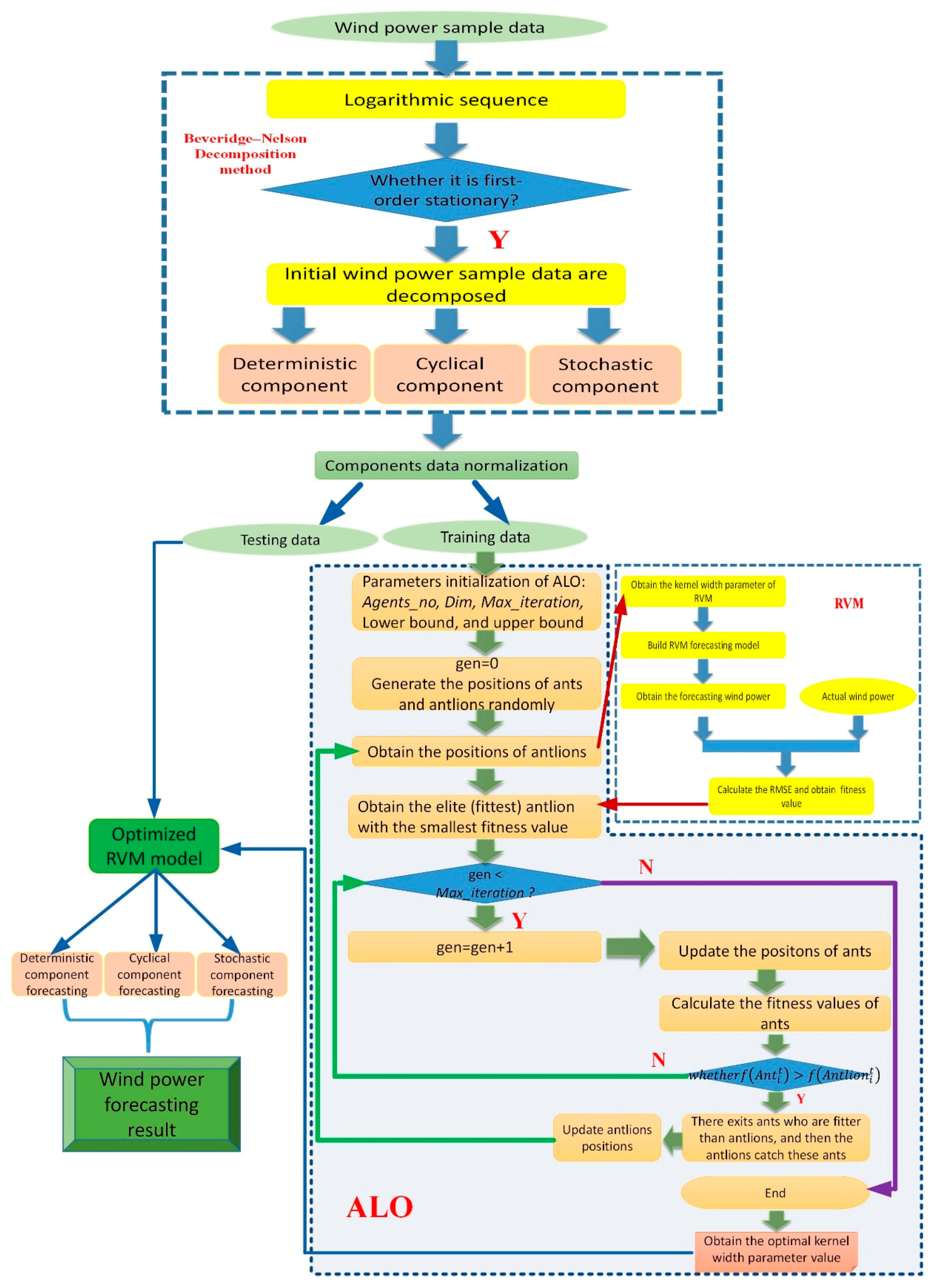
3. The Proposed Hybrid BND-ALO-RVM Forecaster for Wind Power

In this paper, a new hybrid BND-ALO-RVM forecaster is proposed for wind power. Considering the non-stationary characteristics of wind power time series, the BND method is firstly employed to decompose the initial wind power time series into three components: the deterministic, cyclical and stochastic component. Then, the RVM technique is used to forecast these three components, respectively. To improve the forecasting performance, the kernel width parameter $\sigma$ of the RVM model is optimally determined using a new swarm intelligent algorithm ALO. Finally, the forecasted wind power can be obtained by multiplying the forecasting results of three decomposed components.

The detailed procedures of the proposed hybrid BND-ALO-RVM method for wind power forecasting are elaborated as below:

Step 1: Perform unit root test.

When the Beveridge-Nelson decomposition method is used, the first thing is to examine whether the logarithmic sequence of initial wind power time series is first-order stationary or not. If the first-order difference of logarithmic sequence of initial wind power time series is stationary, then we can proceed to the next step. In this paper, the Augmented Dickey-Fuller (ADF) method is used to perform unit root tests.

Step 2: Decompose wind power time series.

Once the condition that the first-order difference of logarithmic sequence of initial wind power data is stationary is confirmed, the wind power time series can be decomposed into the deterministic, cyclical and stochastic components by using the BND method.

Step 3: Set initial parameters.

For the ALO algorithm, five parameters, namely ants and antlion numbers Agents_no, variables number dim, maximum iteration number Max_iteration, lower boundary $lb=\left[l{b}_1,l{b}_2,\cdots \right]$ and upper boundary $ub=\left[u{b}_1,u{b}_2,\cdots \right]$ need to be initially set. In this paper, these five parameters are set as follows: Agents_no = 10, dim = 1, Max_iteration = 100, lb = 0.001, and ub = 100.

Step 4: Start optimization search.

The fitness function $f[\ast ]$ needs to be determined firstly when the ALO is used to optimize the kernel width parameter of RVM. In this study, the root mean square error (RMSE) between actual wind power data and forecasted wind power data is employed to build the fitness function, namely:

$$RMSE=\sqrt{\frac{1}{n}{\displaystyle \sum _{k=1}^n{(x\left(k\right)-\stackrel{\wedge }{x}\left(k\right))}^2}}$$

(33)

where $x\left(k\right)$ is actual wind power data at time k; and $\widehat{x}\left(k\right)$ is the where forecasted wind power value at time k.

The kernel width parameter of RVM is represented by the antlion’s position $M_{Antlion}$, namely each column of $M_{Antlion}$. The optimal position of antlions will be updated at each iteration, and then the optimal kernel width parameter of RVM can be also updated so far. Suppose that the actual wind power decomposition data $\{x^{(0)}(1),x^{(0)}(2),...,x^{(0)}(n)\}$ is used in the first iteration, the forecasted wind power decomposition value $\{{\widehat{x}}^{(0)}(1),{\widehat{x}}^{(0)}(2),...,{\widehat{x}}^{(0)}(n)\}$ can be calculated using the optimized RVM model. At this time, the fitness function and optimization object can be built at this iteration by minimizing RMSE as follows:

$$f=\min \sqrt{\frac{1}{n}{\displaystyle \sum _{k=1}^n{\left(x\left(k\right)-\stackrel{\wedge }{x}\left(k\right)\right)}^2}}$$

(34)

Step 5: Determine the optimal parameter of RVM.

During the iteration and optimization process, different RMSEs will be obtained with different kernel width parameters of RVM. When the iteration reaches a maximum, the minimum RMSE can be found, and then the optimal kernel width parameter σ of RVM can be determined, which will be used for three components forecasting of wind power time series by using the RVM technique.

Step 6: Integrate three components forecasting results and forecast wind power.

After the initial wind power time series are decomposed into three components and the optimal kernel width parameter of RVM is determined, the RVM optimized by ALO will be employed to respectively forecast the three decomposed components, namely the deterministic, cyclical and stochastic component. Then, the forecasting results of these three components are integrated. Finally, the forecasting result of wind power can be obtained by multiplying the forecasting results of the corresponding deterministic, cyclical and stochastic components.

The procedure of the proposed BND-ALO-RVM method used for wind power forecasting in this paper is shown in Figure 1.

4. Empirical Analysis

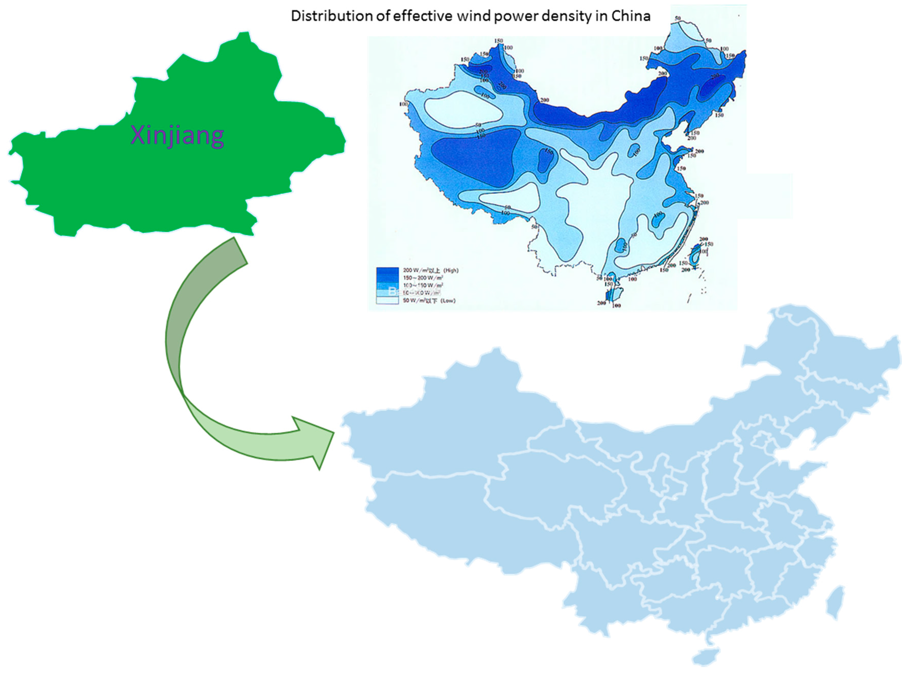
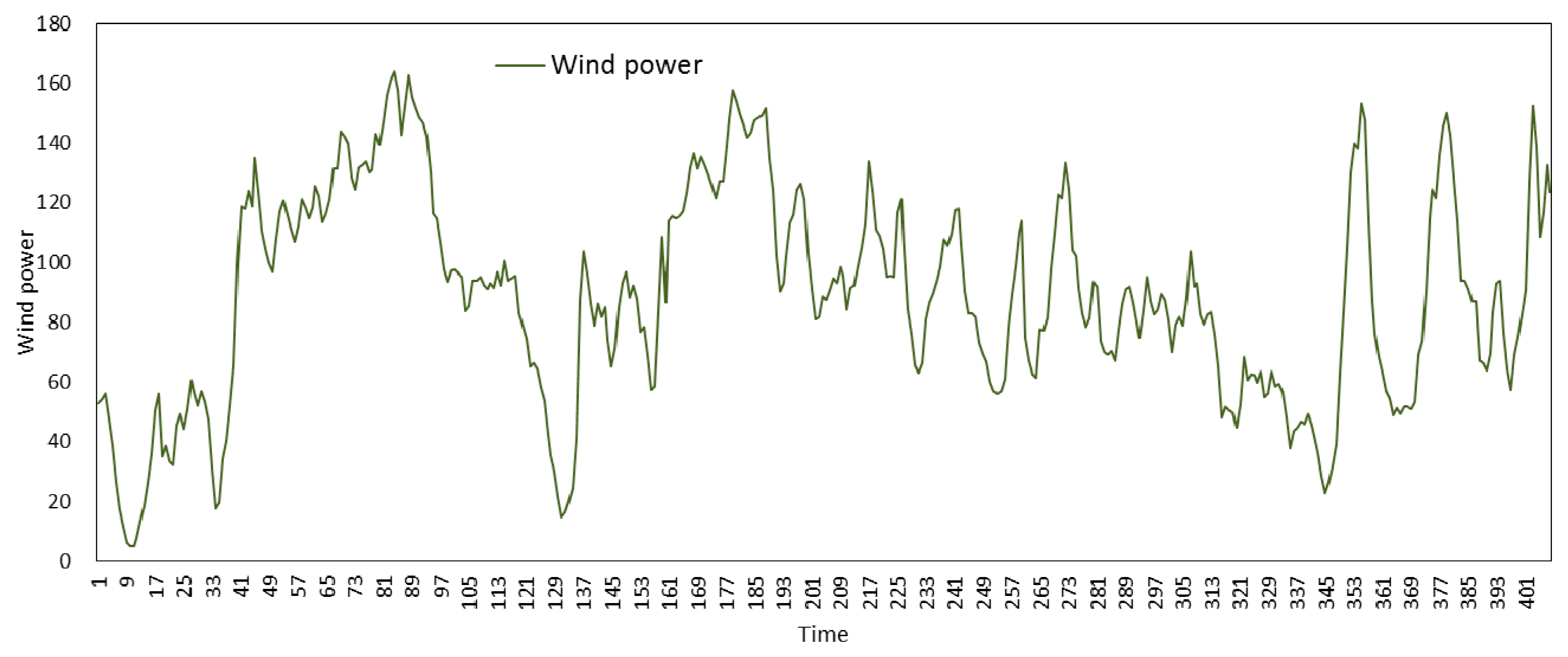
In this paper, hourly wind power from the Xinjiang Uygur autonomous region in China collected during June 2015 was employed for empirical analysis to validate the proposed BND-ALO-RVM forecaster. The Xinjiang Uygur autonomous region, which has plentiful wind resources, is located in the northwest of China, as shown in Figure 2. The sample set in this paper includes 408 hourly wind power points from 14 June to 30 June, which are shown in Figure 3. It can be seen that the wind power, which ranges from about 5 MW to 164 MW, fluctuates greatly. No apparent variation pattern of the wind power time series can be seen.

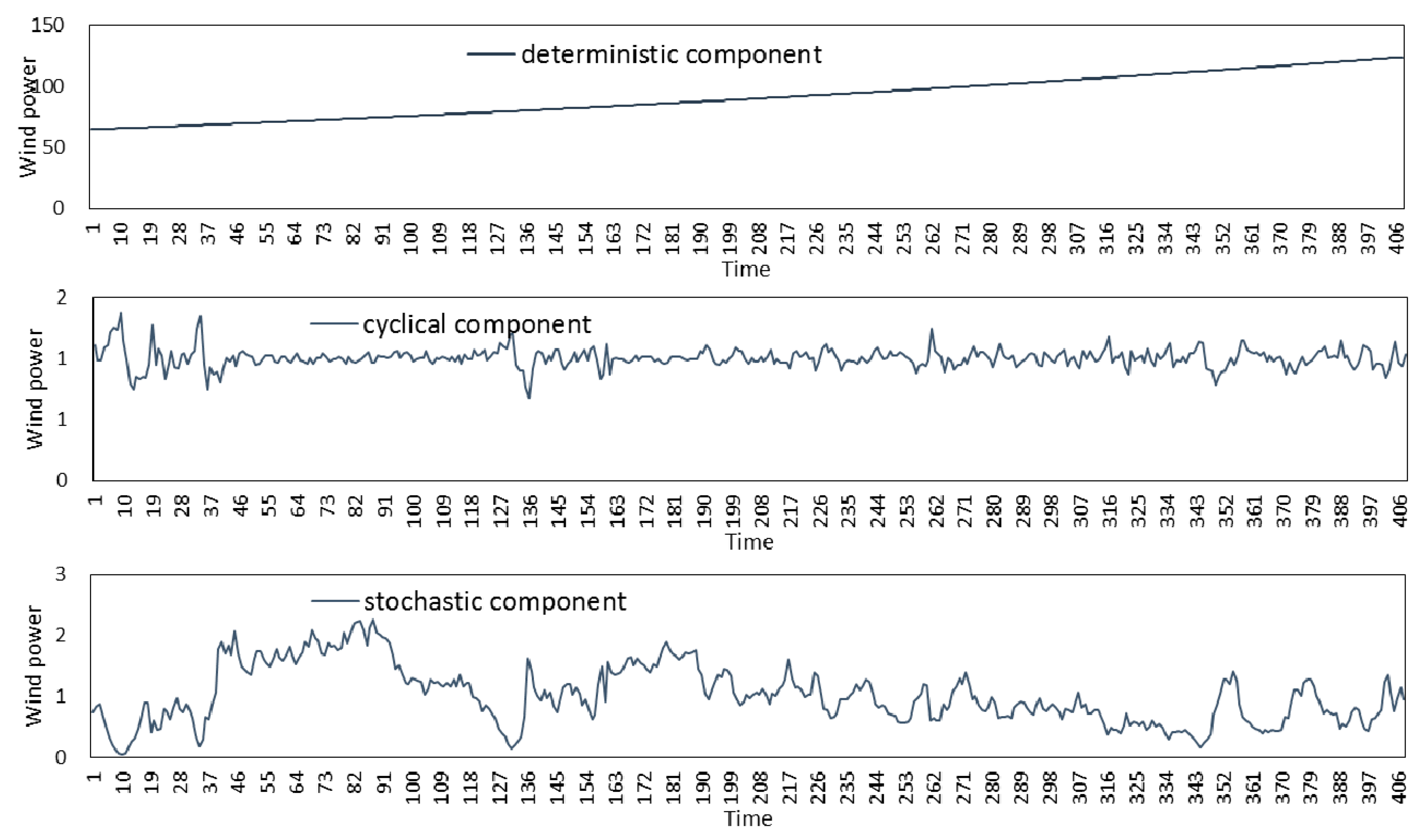
4.1. Wind Power Time Series Decomposition Using BND Method

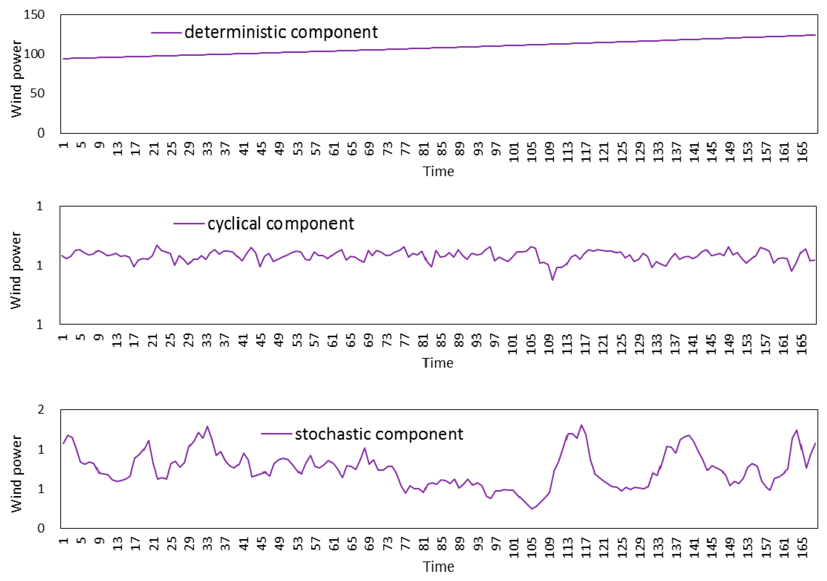
The BND method is applied to decompose the original wind power time series. Before data decomposition, the unit root test based on the ADF test is necessary to judge whether the logarithmic sequence of wind power time series is first-order stationary. The ADF test results are listed in

Table 1. ADF test result of wind power time series.

Sequence	Test Form (C,T,K)	ADF Test Value	P Value	Conclusion
$\ln P$	(N,N,1)	−2.5705	0.1098	Unstable
$\Delta \ln P$	(N,N,0)	−11.5359	0.0000	stable

, where it can be seen that the wind power time series are stable after first-order difference. Then, the BND method can be used to decompose the wind power time series. The decomposition result of the original wind power time series is shown in Figure 4, which includes the deterministic, cyclical and stochastic components.

4.2. Forecasting Results

After the original wind power time series are decomposed, the deterministic, cyclical and stochastic components will be respectively forecasted using ALO-RVM, which means the kernel width parameter of RVM will be respectively optimized and determined by ALO. The sample set of wind power from 14 June to 30 June is divided into a training sample set and a testing sample set. Two hundred and sixteen (216) sample data points of hourly wind power from 14 June to 23 June are used as training sample, and the remaining 168 sample data points from 24 June to 30 June are treated as testing sample.

The inputs of ALO-RVM model are historical hourly wind power 1 h ahead and hourly wind power at the same time yesterday. For example, for forecasting the deterministic component of wind power time series at the 1st hour of 24 June, the deterministic component of wind power time series at 1 h ahead (i.e., deterministic component of the 24th hour wind power data at 23 June) and deterministic component of wind power time series at the same time yesterday (i.e., deterministic component of the 1st hour wind power data at 23 June) will be employed as the input variables. In this way, the deterministic components of wind power time series from the 2nd hour of 24 June to the 24th hour of 30 June can be forecasted. Meanwhile, the cyclical components and stochastic components of the wind power time series from the 1st hour of 24 June to the 24th hour of 30 June can also be forecasted. Finally, the wind power from the 1st hour of 24 June to the 24th hour of 30 June can be respectively obtained by conducting the multiplication of forecasted deterministic components, cyclical components and stochastic components from the 1st hour of 24 June to the 24th hour of 30 June. For the training period, the same way is taken in this paper. The training sample data and testing sample data will be respectively normalized before training and testing by using ALO-RVM method, and the normalization method is as follows:

$$\tilde{x}=\frac{x-x_{\min }}{x_{\max }-x_{\min }}$$

(35)

where $x$ and $\tilde{x}$ are the original and normalized wind power data, respectively; $x_{\max }$ and $x_{\min }$ respectively represent the maximum and minimum value of each input wind power time series.

During the training period, the kernel width parameter of RVM will be optimally determined using the ALO algorithm for the deterministic, cyclical and stochastic components, respectively. The optimal values of RVM kernel width parameter $\sigma$ for the deterministic, cyclical and stochastic components are respectively 29.2504, 0.0137 and 11.8443, which are also the RVM kernel widths for the deterministic, cyclical and stochastic component during the testing period. The forecasting results of the deterministic, cyclical and stochastic component of the hourly wind power from 24 June to 30 June are shown in Figure 5. Then, the hourly wind power from 24 June to 30 June can be forecast by multiplying the forecasted deterministic, cyclical and stochastic components from 24 June to 30 June, which are shown in Figure 6.

4.3. Forecasting Performance Evaluation

To evaluate the forecasting performance of the proposed BND-ALO-RVM forecaster for wind power, four comparison methods are selected, which are single RVM without data decomposition and parameter optimization (referred to as RVM), RVM only with data decomposition using BND (referred to as BND-RVM), RVM only with parameter optimization (referred to as ALO-RVM), and generalized regression neural network with data decomposition using wavelet transform (referred to as WT-GRNN). The input variables and output variable of these four comparing forecasting methods are the same as those of the BDN-ALO-RVM method.

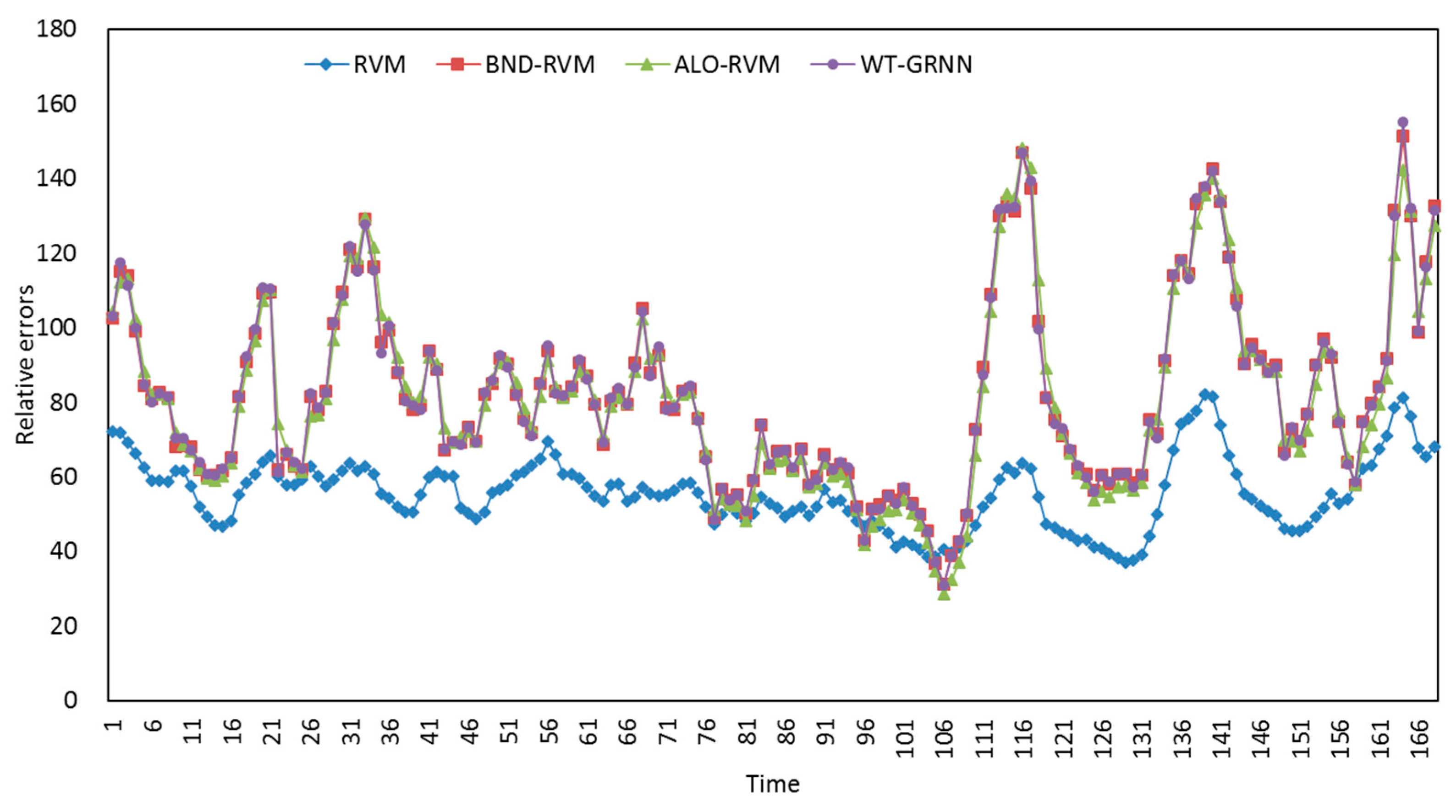
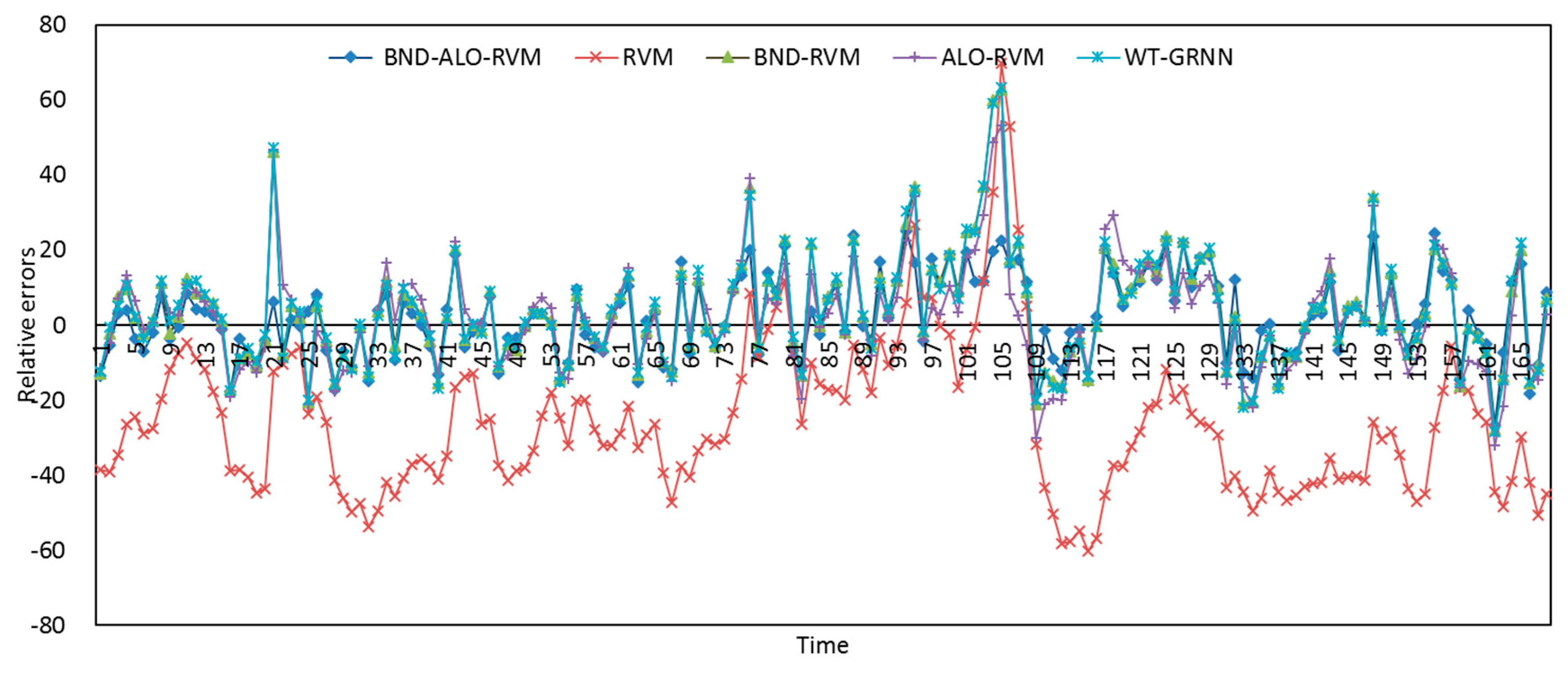
For RVM and BND-RVM, the kernel width parameter is set as 3. For ALO-RVM, through training, the optimal kernel width parameter of RVM is determined as 7.4645. For WT-GRNN, a fast discrete wavelet transform based on four filters developed by Mallat [47] is employed, and the spread parameter value of GRNN is selected as 3. The forecasted hourly wind powers from 24 June to 30 June using RVM, BND-RVM, ALO-RVM, and WT-GRNN are shown in Figure 7. The relative errors of forecasted hourly wind power using BND-ALO-RVM, RVM, BND-RVM, ALO-RVM, and WT-GRNN methods are shown in Figure 8. From Figure 8, it can be roughly seen that the proposed BND-ALO-RVM method has the best forecasting performance due to its much smaller relative errors, and RVM without data decomposition and parameter optimization has the poorest forecasting capacity due to its larger relative errors.

To further compare the forecasting performances of the different methods, three forecasting error criteria are selected to evaluate the forecasting performances of the different models, which are Mean Absolute Percentage Error (MAPE, see Equation (36)), Root Mean Square Error (RMSE) and Mean Absolute Error (MAE, see Equation (37)):

$$MAPE=\frac{1}{n}{\displaystyle \sum _{k=1}^n\left|\frac{x(k)-\widehat{x}(k)}{x(k)}\right|}\times 100\%$$

(36)

$$MAE=\frac{1}{n}{\displaystyle \sum _{k=1}^n\left|x(k)-\widehat{x}(k)\right|}\times 100\%$$

(37)

The MAPEs, RMSEs and MAEs of different forecasting methods, namely BND-ALO-RVM, RVM, BND-RVM, ALO-RVM, and WT-GRNN at each forecasted day are listed in

Table 2. Forecasting performances of different methods.

Methods/Criteria	BND-ALO-RVM			RVM			BND-RVM			ALO-RVM			WT-GRNN
	MAPE (%)	RMSE (MW)	MAE (MW)	MAPE (%)	RMSE (MW)	MAE (MW)	MAPE (%)	RMSE (MW)	MAE (MW)	MAPE (%)	RMSE (MW)	MAE (MW)	MAPE (%)	RMSE (MW)	MAE (MW)
24 June	5.47	6.25	4.71	23.66	26.67	21.41	8.29	9.73	6.71	9.09	10.34	7.46	8.44	9.73	6.65
25 June	7.23	8.56	6.78	35.21	38.18	34.02	7.83	8.97	7.22	8.44	9.86	7.81	7.97	9.26	7.36
26 June	6.87	7.32	5.94	30.84	27.87	26.67	6.76	7.08	5.82	6.94	7.18	5.94	6.92	7.36	5.97
27 June	10.12	6.60	5.46	12.98	9.85	7.89	12.37	8.23	6.60	10.76	7.52	5.77	12.43	8.24	6.64
28 June	12.32	9.49	7.60	33.34	42.69	30.09	19.11	12.26	10.66	17.01	13.99	11.00	18.85	12.30	10.55
29 June	10.69	9.44	8.13	34.50	39.83	33.87	12.01	10.98	9.42	10.73	11.26	9.25	12.07	11.05	9.43
30 June	9.94	12.33	9.40	33.87	38.38	33.54	10.71	13.29	10.12	12.18	15.07	11.37	10.84	13.79	10.35
26–30 June	8.95	8.79	6.86	29.20	33.64	26.79	11.01	10.29	8.08	10.74	11.10	8.37	11.07	10.46	8.13

. From the perspective of average forecasting performance from 24 June to 30 June, the proposed BND-ALO-RVM has the best forecasting performance because it has the minimum MAPE, RMSE and MAE, which are 8.95%, 8.79 MW and 6.86 MW, respectively. The MAPE of BND-ALO-RVM model is (29.20 − 8.95)/29.20 = 69.35%, (11.01 − 8.95)/11.01 = 18.75%, (10.74 − 8.95)/10.74 = 16.66%, and (11.07 − 8.95)/11.07 = 19.15% lower than that of RVM, BND-RVM, ALO-RVM, and WT-GRNN, respectively. The RMSE of BND-ALO-RVM model is (33.64 − 8.79)/33.64 = 73.89%, (10.29 − 8.79)/10.29 = 14.58%, (11.10 − 8.79)/11.10 = 20.81%, and (10.46 − 8.79)/10.46 = 15.97% lower than that of RVM, BND-RVM, ALO-RVM, and WT-GRNN, respectively. The MAE of BND-ALO-RVM model is (26.79 − 6.86)/26.79 = 74.39%, (8.08 − 6.86)/8.08 = 15.07%, (8.37 − 6.86)/8.37 = 18.05%, and (8.13 − 6.86)/8.13 = 15.62% lower than that of RVM, BND-RVM, ALO-RVM, and WT-GRNN, respectively. Therefore, it can be seen that the proposed BDN-ALO-RVM method has the best forecasting performance in terms of short-term wind power, and the single RVM has the worst forecasting performance. The MAPE of BND-RVM is larger than that of ALO-RVM, but smaller than that of WT-GRNN. The RMSE and MAE of BND-RVM are both smaller than that of ALO-RVM and WT-GRNN. Therefore, it can be said that the forecasting performance of BND-RVM is better than that of WT-GRNN, but it is hard to say which is better between BND-RVM and ALO-RVM. The MAPE of ALO-RVM is smaller than that of WT-GRNN, but the RMSE and MAE of ALO-RVM are larger than that of ALO-RVM, so for ALO-RVM and WT-GRNN, we cannot decide in this paper which one is better in term of wind power forecasting.

From the perspective of forecasting performance during each day, the proposed BDN-ALO-RVM method obtains the smallest MAPEs, RMSEs and MAEs among all five forecasting models on 24 June, 25 June, 27 June, 28 June, 29 June and 30 June. On 26 June, the BND-RVM obtains the smallest MAPE, RMSE, and MAE. The RVM model gets the largest MAPE, RMSE, and MAE on each day between 24 June and 30 June, which indicates it has the worst forecasting performance again. This is because the RVM without data decomposition and parameter optimization cannot grasp the characteristics of wind power time series. The forecasting performance of BND-RVM method is better than single RVM because BND-RVM method obtains smaller MAPEs, RMSEs and MAEs, which indicates BND is an effective wind power time series decomposition method to improve the wind power forecasting accuracy. Meanwhile, the forecasting performance of the ALO-RVM method is better than single RVM, which indicates the ALO is an effective algorithm for kernel width parameter optimization of RVM to improve the wind power forecasting accuracy. For BND-RVM and ALO-RVM methods, the BND-RVM method has better forecasting performance than ALO-RVM on 24 June, 25 June, 26 June and 30 June, and the ALO-RVM has better forecasting performance than BND-RVM on 27 June. It is hard to judge which one has better forecasting performance between BND-RVM and ALO-RVM because the different rankings related to MAPEs, RMSEs, and MAEs on 28 June and 29 June. For BND-RVM and WT-GRNN methods, except the MAE criterion on 24 June and 28 as well as MAPE criterion on 28 June, the BND-RVM shows better forecasting performance than WT-GRNN. On the whole, the BND-RVM has better forecasting performance than WT-GRNN, which indicates the BND employed in this paper is an effective technique for wind power time series decomposition.

To sum up the above analysis, we can conclude that the proposed BDN-ALO-RVM forecaster is an effective and applicable technique, which can improve the forecasting accuracy of hourly wind power. Meanwhile, the BND method is a valid wind power time series decomposition technique, and ALO is an efficient meta-heuristic algorithm for kernel width parameter determination of RVM in the field of wind power forecasting.

5. Conclusions

Wind power is a kind of environmentally friendly renewable energy power, which has developed rapidly in recent years. However, the large-scale penetration of wind power with its stochastic and intermittent characteristics into electric power systems will pose some threats to the stable and safe operation of these systems. Improving wind power forecasting accuracy can alleviate these threats. Therefore, a new hybrid BND-ALO-RVM forecaster for wind power is proposed in this paper, which combines the Beveridge-Nelson decomposition method, relevance vector machine and ant lion optimizer. The wind power time series are firstly decomposed into deterministic, cyclical and stochastic components. Then, these three decomposed components are respectively forecasted by using ALO-RVM method, which mean that the kernel width parameter of RVM is optimally determined by the ALO algorithm. Finally, the wind power forecasting results can be obtained by multiplying the forecasted deterministic, cyclical and stochastic components. Taking hourly wind power from the Xinjiang Uygur autonomous region in China as an example, the empirical results indicate the proposed BND-ALO-RVM forecaster obtains the best forecasting performance compared with the single RVM, BND-RVM, ALO-RVM, and WT-GRNN methods. The proposed BND-ALO-RVM method has the minimum MAPE, RMSE and MAE, which are 8.95%, 8.79 MW and 6.86 MW, respectively. However, MAPE, RMSE and MAE of single RVM method are respectively 29.20%, 33.64 MW and 26.79 MW; MAPE, RMSE and MAE of BND-RVM method are respectively 11.01%, 10.29 MW and 8.08 MW; MAPE, RMSE and MAE of ALO-RVM method are respectively 10.74%, 11.10 MW and 8.37 MW; and MAPE, RMSE and MAE of BND-RVM method are respectively 11.07%, 10.46 MW and 8.13 MW. The proposed BND-ALO-RVM method is effective and practical for short-term wind power forecasting. The BND method is a valid wind power time series decomposition technique, and ALO is an attractive meta-heuristic algorithm for RVM parameter determination. This paper enriches the methodology library related to wind power forecasting, and also extends the application domains of BDN and ALO. In future research, the proposed BND-ALO-RVM method may also be employed for other issues, such as photovoltaic power forecasting and power load forecasting.

References

- Zhao, H.-R.; Guo, S.; Fu, L.-W. Review on the costs and benefits of renewable energy power subsidy in China. Renew. Sustain. Energy Rev. 2014, 37, 538–549. [Google Scholar] [CrossRef]
- Kang, J.; Yuan, J.; Hu, Z.; Xu, Y. Review on wind power development and relevant policies in China during the 11th Five-Year-Plan period. Renew. Sustain. Energy Rev. 2012, 16, 1907–1915. [Google Scholar] [CrossRef]
- Hitaj, C. Wind power development in the United States. J. Environ. Econ. Manag. 2013, 65, 394–410. [Google Scholar] [CrossRef]
- Wang, J.; Botterud, A.; Bessa, R.; Keko, H.; Carvalho, L.; Issicaba, D.; Sumaili, J.; Miranda, V. Wind power forecasting uncertainty and unit commitment. Appl. Energy 2011, 88, 4014–4023. [Google Scholar] [CrossRef]
- Aigner, T.; Jaehnert, S.; Doorman, G.L.; Gjengedal, T. The effect of large-scale wind power on system balancing in Northern Europe. IEEE Trans. Sustain. Energy 2012, 3, 751–759. [Google Scholar] [CrossRef]
- Ortega-Vazquez, M.A.; Kirschen, D.S. Assessing the impact of wind power generation on operating costs. IEEE Trans. Smart Grid 2010, 1, 295–301. [Google Scholar] [CrossRef]
- Ummels, B.C.; Gibescu, M.; Pelgrum, E.; Kling, W.L.; Brand, A.J. Impacts of wind power on thermal generation unit commitment and dispatch. IEEE Trans. Energy Convers. 2007, 22, 44–51. [Google Scholar] [CrossRef]
- Soman, S.S.; Zareipour, H.; Malik, O.; Mandal, P. A Review of Wind Power and Wind Speed Forecasting Methods with Different Time Horizons. In Proceedings of the North American Power Symposium (NAPS 2010), Arlington, TX, USA, 26–28 September 2010; Institute of Electrical and Electronics Engineers: New York, NY, USA, 2010; pp. 1–8. [Google Scholar]
- Costa, A.; Crespo, A.; Navarro, J.; Lizcano, G.; Madsen, H.; Feitosa, E. A review on the young history of the wind power short-term prediction. Renew. Sustain. Energy Rev. 2008, 12, 1725–1744. [Google Scholar] [CrossRef]
- Lange, M.; Focken, U. Physical Approach to Short-Term Wind Power Prediction; Springer: New York, NY, USA, 2006. [Google Scholar]
- Landberg, L.; Watson, S.J. Short-term prediction of local wind conditions. Bound. Layer Meteorol. 1994, 70, 171–195. [Google Scholar] [CrossRef]
- Focken, U.; Lange, M.; Waldl, H.-P. Previento-A wind power prediction system with an innovative upscaling algorithm. In Proceedings of the European Wind Energy Conference, Copenhagen, Denmark, 2–6 July 2001. [Google Scholar]
- McGowin, C. California Wind Energy Forecasting System Development and Testing. Phase 1: Initial Testing; EPRI Final Report; Electric Power Reserach Institute: Palo Alto, CA, USA, 2003. [Google Scholar]
- Erdem, E.; Shi, J. ARMA based approaches for forecasting the tuple of wind speed and direction. Appl. Energy 2011, 88, 1405–1414. [Google Scholar] [CrossRef]
- Torres, J.L.; Garcia, A.; de Blas, M.; de Francisco, A. Forecast of hourly average wind speed with ARMA models in Navarre (Spain). Sol. Energy 2005, 79, 65–77. [Google Scholar] [CrossRef]
- Kavasseri, R.G.; Seetharaman, K. Day-ahead wind speed forecasting using f-ARIMA models. Renew. Energy 2009, 34, 1388–1393. [Google Scholar] [CrossRef]
- Li, G.; Shi, J. On comparing three artificial neural networks for wind speed forecasting. Appl. Energy 2010, 87, 2313–2320. [Google Scholar] [CrossRef]
- Barbounis, T.G.; Theocharis, J.B.; Alexiadis, M.C.; Dokopoulos, P.S. Long-term wind speed and power forecasting using local recurrent neural network models. IEEE Trans. Energy Convers. 2006, 21, 273–284. [Google Scholar] [CrossRef]
- Liu, Y.; Shi, J.; Yang, Y.; Lee, W.-J. Short-term wind-power prediction based on wavelet transform–support vector machine and statistic-characteristics analysis. IEEE Trans. Ind. Appl. 2012, 48, 1136–1141. [Google Scholar] [CrossRef]
- Wan, C.; Xu, Z.; Pinson, P.; Dong, Z.Y.; Wong, K.P. Probabilistic forecasting of wind power generation using extreme learning machine. IEEE Trans. Power Syst. 2014, 29, 1033–1044. [Google Scholar] [CrossRef]
- Mohammadi, K.; Shamshirband, S.; Yee, L.; Petković, D.; Zamani, M.; Ch, S. Predicting the wind power density based upon extreme learning machine. Energy 2015, 86, 232–239. [Google Scholar] [CrossRef]
- Ren, C.; An, N.; Wang, J.; Li, L.; Hu, B.; Shang, D. Optimal parameters selection for BP neural network based on particle swarm optimization: A case study of wind speed forecasting. Knowl. Based Syst. 2014, 56, 226–239. [Google Scholar] [CrossRef]
- Amjady, N.; Keynia, F.; Zareipour, H. Wind power prediction by a new forecast engine composed of modified hybrid neural network and enhanced particle swarm optimization. IEEE Trans. Sustain. Energy 2011, 2, 265–276. [Google Scholar] [CrossRef]
- Jursa, R.; Rohrig, K. Short-term wind power forecasting using evolutionary algorithms for the automated specification of artificial intelligence models. Int. J. Forecast. 2008, 24, 694–709. [Google Scholar] [CrossRef]
- Liu, D.; Niu, D.; Wang, H.; Fan, L. Short-term wind speed forecasting using wavelet transform and support vector machines optimized by genetic algorithm. Renew. Energy 2014, 62, 592–597. [Google Scholar] [CrossRef]
- Salcedo-Sanz, S.; Pastor-Sánchez, A.; Prieto, L.; Blanco-Aguilera, A.; García-Herrera, R. Feature selection in wind speed prediction systems based on a hybrid coral reefs optimization–Extreme learning machine approach. Energy Convers. Manag. 2014, 87, 10–18. [Google Scholar] [CrossRef]
- Foley, A.M.; Leahy, P.G.; Marvuglia, A.; McKeogh, E.J. Current methods and advances in forecasting of wind power generation. Renew. Energy 2012, 37, 1–8. [Google Scholar] [CrossRef]
- Osório, G.; Matias, J.; Catalão, J. Short-term wind power forecasting using adaptive neuro-fuzzy inference system combined with evolutionary particle swarm optimization, wavelet transform and mutual information. Renew. Energy 2015, 75, 301–307. [Google Scholar] [CrossRef]
- Haque, A.U.; Mandal, P.; Meng, J.; Srivastava, A.K.; Tseng, T.-L.; Senjyu, T. A novel hybrid approach based on wavelet transform and fuzzy ARTMAP networks for predicting wind farm power production. IEEE Trans. Ind. Appl. 2013, 49, 2253–2261. [Google Scholar] [CrossRef]
- Ren, Y.; Suganthan, P.; Srikanth, N. A comparative study of empirical mode decomposition-based short-term wind speed forecasting methods. IEEE Trans. Sustain. Energy 2015, 6, 236–244. [Google Scholar] [CrossRef]
- Liu, H.; Tian, H.; Liang, X.; Li, Y. New wind speed forecasting approaches using fast ensemble empirical model decomposition, genetic algorithm, Mind Evolutionary Algorithm and Artificial Neural Networks. Renew. Energy 2015, 83, 1066–1075. [Google Scholar] [CrossRef]
- Beveridge, S.; Nelson, C.R. A new approach to decomposition of economic time series into permanent and transitory components with particular attention to measurement of the ‘business cycle’. J. Monet. Econ. 1981, 7, 151–174. [Google Scholar] [CrossRef]
- Zarnowitz, V.; Ozyildirim, A. Time series decomposition and measurement of business cycles, trends and growth cycles. J. Monet. Econ. 2006, 53, 1717–1739. [Google Scholar] [CrossRef]
- Cochrane, J.H. Permanent and transitory components of GNP and stock prices. Q. J. Econ. 1994, 109, 241–265. [Google Scholar] [CrossRef]
- Carlino, G.; Sill, K. Regional income fluctuations: Common trends and common cycles. Rev. Econ. Stat. 2001, 83, 446–456. [Google Scholar] [CrossRef]
- Yan, J.; Liu, Y.; Han, S.; Qiu, M. Wind power grouping forecasts and its uncertainty analysis using optimized relevance vector machine. Renew. Sustain Energy Rev. 2013, 27, 613–621. [Google Scholar] [CrossRef]
- Matsumoto, M.; Hori, J. Classification of silent speech using support vector machine and relevance vector machine. Appl. Soft Comput. 2014, 20, 95–102. [Google Scholar] [CrossRef]
- Li, H.; Pan, D.; Chen, C.P. Intelligent prognostics for battery health monitoring using the mean entropy and relevance vector machine. IEEE Trans. Syst. Man Cybern. Syst. 2014, 44, 851–862. [Google Scholar] [CrossRef]
- Flake, J.; Moon, T.K.; McKee, M.; Gunther, J.H. Application of the relevance vector machine to canal flow prediction in the Sevier River Basin. Agric. Water Manag. 2010, 97, 208–214. [Google Scholar] [CrossRef]
- Torres, A.F.; Walker, W.R.; McKee, M. Forecasting daily potential evapotranspiration using machine learning and limited climatic data. Agric. Water Manag. 2011, 98, 553–562. [Google Scholar] [CrossRef]
- Wang, T.; Xu, H.; Han, J.; Elbouchikhi, E.; Benbouzid, M.E.H. Cascaded H-bridge multilevel inverter system fault diagnosis using a PCA and multiclass relevance vector machine approach. IEEE Trans. Power Electron. 2015, 30, 7006–7018. [Google Scholar] [CrossRef]
- Mirjalili, S. The ant lion optimizer. Adv. Eng. Softw. 2015, 83, 80–98. [Google Scholar] [CrossRef]
- Zhao, H.; Guo, S. An optimized grey model for annual power load forecasting. Energy 2016, 107, 272–286. [Google Scholar] [CrossRef]
- Morley, J.C. A state-space approach to calculating the Beveridge-Nelson decomposition. Econ. Lett. 2002, 75, 123–127. [Google Scholar] [CrossRef]
- Newbold, P. Precise and efficient computation of the Beveridge-Nelson decomposition of economic time series. J. Monét. Econ. 1990, 26, 453–457. [Google Scholar] [CrossRef]
- Tipping, M.E. Sparse Bayesian learning and the relevance vector machine. J. Mach. Learn. Res. 2001, 1, 211–244. [Google Scholar]
- Mallat, S.G. A theory for multiresolution signal decomposition: The wavelet representation. IEEE Trans. Pattern Anal. Mach. Inell. 1989, 11, 674–693. [Google Scholar] [CrossRef]
Figure 1.
Flowchart of the proposed BND-ALO-RVM wind power forecaster.
Figure 2.
Geographical location of Xinjiang and its wind resources.
Figure 3.
Wind power time series from 14 June to 30 June (408 sample points).
Figure 4.
Decomposed deterministic component, cyclical component and stochastic component of the original wind power time series.
Figure 5.
Forecasted deterministic component, cyclical component and stochastic component of the wind power time series from 24 June to 30 June.
Figure 6.
Forecasting result of wind power from 24 June to 30 June.
Figure 7.
Forecasting results of hourly wind power by using different comparison methods.
Figure 8.
Relative errors of the forecasted hourly wind power of different methods.