A Novel Sectionalizing Method for Power System Parallel Restoration Based on Minimum Spanning Tree


School of Electrical Engineering, Beijing Jiaotong University, Beijing 100044, China; [email protected] (C.L.); [email protected] (J.H.); [email protected] (P.Z.)
*
Author to whom correspondence should be addressed.
Energies 2017, 10(7), 948; https://doi.org/10.3390/en10070948
Submission received: 4 May 2017
/
Revised: 3 July 2017
/
Accepted: 4 July 2017
/
Published: 8 July 2017
(This article belongs to the Section F: Electrical Engineering)
Abstract
:Parallel restoration is a way to accelerate the black-start procedure of power systems following a blackout. An efficient sectionalizing scheme can reduce the restoration time of a system, taking into account the black-start ability, generation-load balance of subsystems, restoration time of branches, start-up time of generating units, and effects of dispatchable loads and faulted devices. Solving the sectionalizing problem is challenging since it needs to handle a large number of Boolean variables corresponding to the branches and nonlinear constraints associated with system topology. This paper investigates power system sectionalizing problem for parallel restoration to minimize the system restoration time (SRT). A novel sectionalizing method considering the restoration of generating units and network branches is proposed. Firstly, the minimum spanning tree (MST) algorithm is used to determine the skeleton network of a power system. Secondly, the number of subsystems is determined according to the number of black-start units. Based on the skeleton network, candidate boundary lines among subsystems are identified. Then, constraints are evaluated to identify feasible sectionalizing schemes. Except commonly used constraints on power balancing and black-start units, this paper also considers using dispatchable loads to meet the minimum output requirements of generating units. Finally, the sectionalizing scheme with the minimum SRT is selected as the final solution. The effectiveness of the proposed method is validated by the IEEE 39-bus and 118-bus test systems. The simulation results indicate that the proposed method can balance the restoration time of subsystems and minimize the SRT.
1. Introduction
Several major blackouts occurred worldwide in the past few decades, e.g., the 14 August 2003 blackout in the northern USA and Canada [1], the 4 November 2006 blackout in Western Europe [2], the 30–31 July 2012 blackout in India [3] and the 31 March 2015 blackout in Turkey [4]. A major blackout, caused by natural disasters, cascading failures or human errors, threatens the security and reliability of power systems and has negative impacts on social and economic development [5,6]. A more secure and reliable power system considering the severe weather and multiple contingencies is required [7,8,9]. The task of power system restoration is to restore the outage system quickly and safely. Therefore, efficient restoration strategies receive increasing attentions from the power industry [10,11].
The primary goal of system restoration is to restore generating units and loads, and recover the transmission network quickly [12,13,14,15,16]. Parallel restoration strategies, which sectionalize a power system into several subsystems and restore these subsystems simultaneously, are preferred since it accelerates the system restoration process. The first step for parallel restoration is to determine a sectionalizing scheme. Some utilities and ISOs, including PJM (Pennsylvania–New Jersey–Maryland Interconnection) in United States [17], National Grid Company in United Kingdom [18] and Chongqing Power of China State Grid [19], have adopted parallel restoration plans for their systems. The sectionalizing schemes are designed mainly based on the operators’ knowledge and experience.
In recent years, theoretical investigations on sectionalizing methods for parallel restoration have attracted researchers’ interests. The sectionalizing problem, which is usually determined by solving an optimization problem with constraints on black-start generators and generation-load imbalance, is proved to be a non-deterministic polynomial complete problem (NP-complete) [20]. There is no polynomial-time algorithm to solve it. Thus, it is difficult and time consuming to solve the sectionalizing problem for large-scale power systems. Wang, C. et al. applied the ordered binary decision diagram-based method (OBDD) to reduce the candidate sectionalizing schemes for determining optimal solution [20]. Afrakhte et al. applied genetic algorithm (GA) to find the subsystem boundaries and minimize the index of energy not supplied (ENS) [21]. Liang et al. also used GA to create subsystems with consideration of the start-up sequence of units [22]. Quiros-Tortos et al. put forward a sectionalizing methodology based on the cut-set matrix theory [23]. It was simple and useful for parallel restoration. Based on it, Sun et al. developed an optimal network sectionalizing strategy considering cranking generating units [24]. To minimize the time of units for getting cranking power is one of its objectives. These two methods are based on the recursive bisection and obtain two new subsystems by one iteration. After multiple iterations, multiple subsystems can be generated. Sarmadi et al. proposed a heuristic search algorithm to define an islands’ matrix [25]. Considering the wide area measurement system (WAMS) information, the partitioning scheme for parallel restoration is determined by modifying the islands’ matrix. A community detection algorithm was employed into the sectionalizing method for parallel restoration by Lin et al. [26]. The method can also generate the sequence for resynchronization of subsystems. The spectral graph clustering method was used in [27,28] to design the optimal sectionalizing schemes. The sectionalized results depended on the eigenvalues of the Laplacian matrix of the system network, which were the impedance characteristics of branches.
The aforementioned methods are focused on the topology of system without consideration of restoration time of the subsystems. A practical and efficient sectionalizing scheme can reduce the system restoration time (SRT) of a power system, which depends on the subsystem with the slowest restoration process, and enhance the efficiency of parallel restoration. Therefore, the restoration time of each subsystem is an important basis for determining sectionalizing schemes and should be estimated. Adibi discussed the estimation of the restoration duration [29]. The start-up time of generating units and the restoration time of branches are the main time consumption for restoring a power system. The time for the load pick up is ignored [30,31].
The constraints, which should be considered in the sectionalizing problem, are summarized in references [20,21,23]. One important constraint is the minimum active power output of generating units, such as thermal units. To meet the minimum output constraint on generating units, researches generally take the total amount of load as the constraint but have not considered the effects of dispatchable loads [24,25]. Since dispatchable loads can provide the variable power demand, they are widely used in power system operation, e.g., in demand side management [32,33]. For power system restoration, they can be restored flexibly to balance the output of generating units [30,34]. Especially, during the start-up process, a generator cannot be controlled effectively since its control system is designed for use between minimum and maximum load [12]. In this stage, dispatchable loads can be picked up to balance the output of restored units for system security.
This paper proposes a novel sectionalizing method for parallel restoration based on the minimum spanning tree (MST). The objective is to minimize the SRT, considering the start-up time of generating units and the restoration time of branches. A power system can be abstracted as a weighted graph. The weight of each edge, representing a transmission line or a transformer, is specified with its restoration time. For a generating unit, a virtual node and a virtual edge are added. The weight of the virtual edge is set as the start-up time of the unit. Since the MST is a spanning tree with the minimum total weight of edges in a graph, it can determine the skeleton network, which is a minimum adequate network connecting all available buses [30], with the minimum restoration time of the power system. The effect of dispatchable loads is also considered in this paper. Our method offers some distinct advantages:
- (1)
- The start-up time of generating units and the restoration time of branches are considered in the problem formulation, which help minimize the SRT.
- (2)
- By employing the dispatchable loads as an important constraint, it ensures that generating units are restored safely.
- (3)
- Candidate boundary lines of a system are identified according to the skeleton network and used to generate candidate sectionalizing schemes. Expansion in system size will not significantly increase the complexity of the proposed method.
- (4)
- It can be applied to power systems under various conditions, including the conditions when some components are not available, and provide multiple schemes for dispatchers.
2. Problem Formulation
2.1. Objective
A practical and efficient sectionalizing scheme for parallel restoration is to minimize the SRT. Parallel restoration process comprises two stages in general: restoration independently in each subsystem and resynchronization of subsystems. The duration of the first stage, involving the complex operations for restarting generating units, energizing the skeleton transmission network and picking up loads, is the major part of the time consumption for parallel restoration, which usually takes several hours [13,14]. The major work for resynchronization of subsystems is to reduce the phase-angle difference between two subsystems [35,36]. It usually takes about half an hour or less [14,27]. Therefore, the SRT of parallel restoration is evaluated by the duration of the first stage ignoring the time consumption of the second stage in this paper. The sectionalizing objective function is to minimize the SRT, i.e.,
where is the number of subsystems; and represents the restoration time of subsystem . Note that the system restoration duration is mainly determined by the restoration of generating units and branches [29]. Thus, the restoration time of a subsystem is constituted by the start-up time of generating units and the restoration time of skeleton transmission paths within the same subsystem.
2.2. Constraints
2.2.1. Constraint on the Number of Subsystems
To restore each subsystem in parallel, there must be at least one black-start generating unit to supply cranking power for non-black-start units through available transmission paths. There must be loads for balancing the output of generating units in the same subsystem. Generally, the number of non-black-start generating units or loads is much larger than that of black-start generating units in a power system. Therefore, the number of subsystems depends on the number of black-start units, i.e.,
where is the number of black-start generating units.
2.2.2. Minimum Output Constraint on Generating Units
For a generating unit, the minimum output active power is one of key characteristics and determined by technical conditions, such as the fuel combustion stability, and the mechanical considerations of control systems [13,37,38]. Generating units cannot be operated stably at the output lower than their minimum output power. Thus, the demands of loads should not be less than the minimum output of generating units in the same subsystem [24,25].
Loads are constituted by critical loads and non-critical loads. Outages of critical loads, such as hospitals and data centers, may lead to economic losses and negative social impacts. Generally, they must be restored completely and quickly following the stable operation of generating units [30,39]. However, in the stage of the start-up or under low-output conditions of generating units, critical loads should not be picked up to avoid a second failure. The dispatchable loads are non-critical and can be used to provide the required variable capacity to balance the output of restored generating units and improve the controllability of the system [30,34]. Therefore, sufficient dispatchable loads should be guaranteed in subsystem , i.e.,
where is the total minimum output of the generating units at bus ; represents the total active power demand of the dispatchable loads at bus ; and denotes the number of buses in subsystem .
2.2.3. Capacity Constraint on Generating Units
The active power generation capacity depends on all the generating units in each subsystem. To keep the ability of the frequency regulation, sufficient generation capacity margin should be guaranteed during restoration process of each subsystem [24,40]. As the priority of critical loads is high, to restore them is a primary goal of system restoration. All critical loads should be restored before the resynchronization of subsystems. Thus, the following constraint should be accommodated for subsystem
where is the total active power capacity of the generating units at bus ; and is the total active power demand of the critical loads at bus .
2.2.4. Constraint on Faulted Devices
Some devices may be damaged at the time of a blackout. It takes too much time to repair or replace them. Therefore, the disabled devices are not available during the restoration process. For example, the faulted lines cannot be treated as the boundary lines between subsystems.
where is the set of faulted devices and is the set of devices available for restoration.
3. The Proposed Method for Sectionalizing
In this section, a sectionalizing method based on the MST for power system parallel restoration is proposed. Section 3.1 introduces the overall procedure to generate sectionalizing schemes, which consists of four steps. Section 3.2, Section 3.3, Section 3.4 and Section 3.5 illustrate the steps in detail.
3.1. Procedure of the Proposed Sectionalizing Method
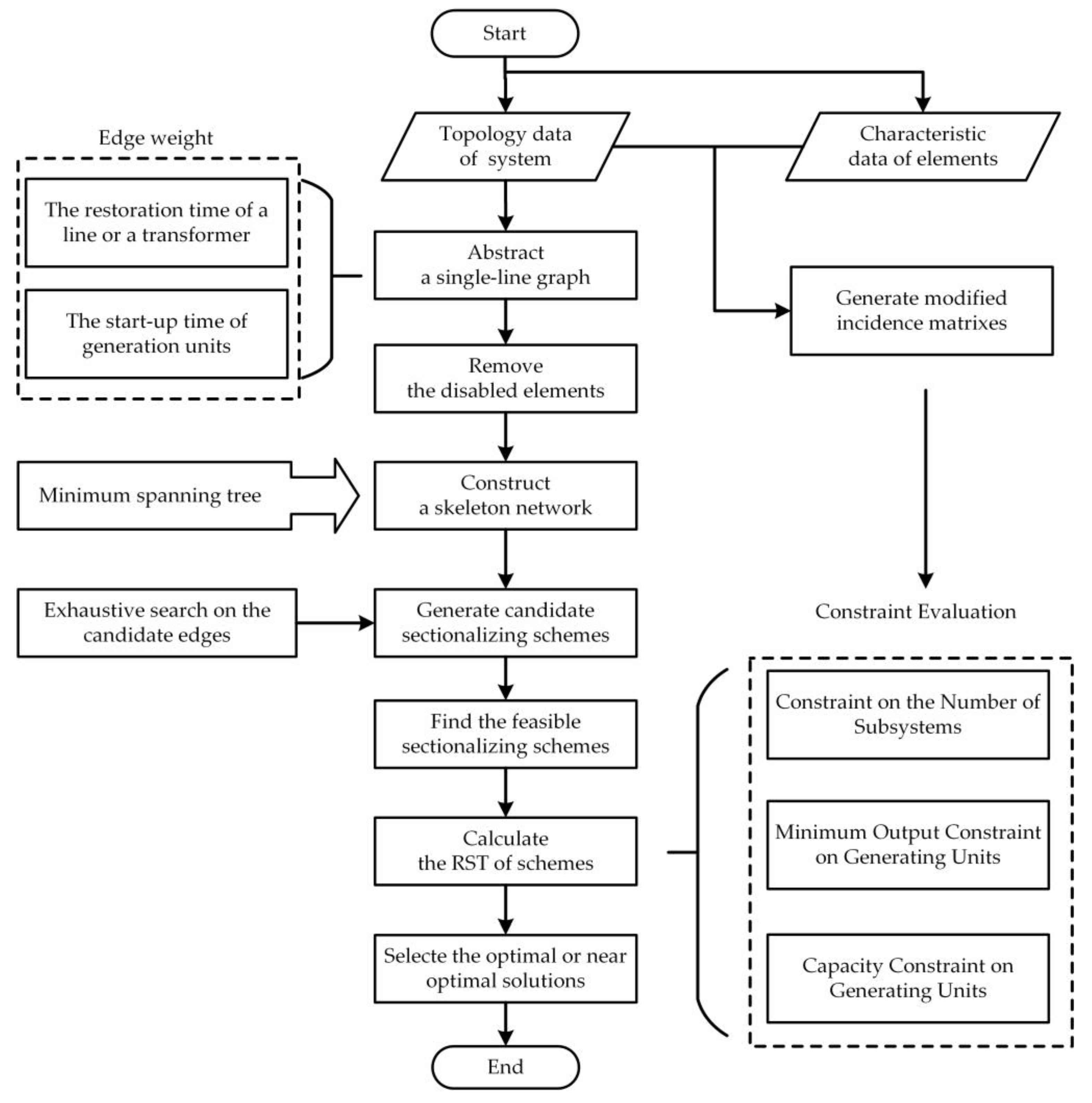
A four-step method is proposed to provide sectionalizing schemes for power system parallel restoration: (1) construct the skeleton network; (2) generate candidate sectionalizing schemes; (3) evaluate constraints; and (4) determine optimal or near-optimal schemes. The flow diagram of the proposed method is shown in Figure 1.
The first step abstracts a power system as a graph. Faulted devices of the system are removed from the graph in order to meet Equation (5). Based on MST, a skeleton network of the graph is constructed considering the start-up time of generating units and the restoration time of branches.
The second step generates candidate sectionalizing schemes by exhaustive search. For each scheme, the skeleton network is divided into several sub-networks. Each sub-network can be used for estimating the total restoration time of the corresponding subsystem. In a subsystem, sequential restoration strategies, i.e., restoring outage elements one-by-one from a black-start unit, are usually adopted. Thus, there must be at least one black-start unit to provide cranking power in each subsystem. In order to accelerate the restoration process and shorten the outage time, it is preferred to have as many subsystems as possible. In this paper, it is assumed that each subsystem contains only one black-start unit. Therefore, the maximum number of subsystems is achieved and equals the number of black-start units.
The third step is aimed at finding the feasible sectionalizing schemes by examining Equations (2)–(4). These constraints are formulated as three inequalities. Details are provided in Section 3.4.
The fourth step calculates the SRT of each sectionalizing scheme. In a scheme, the estimation of restoration time depends on the subsystem with the slowest restoration process. The scheme, which consumes the minimum SRT, is selected as the final sectionalizing solution.
3.2. Constructing the Skeleton Network Based on Minimum Spanning Tree
3.2.1. Abstraction of a Power System
A power system can be described as a weighted connected graph . Generating-unit, substation and load buses of a power system are modeled as nodes, i.e., vertices in the graph. For each generating unit, a virtual node, as well as a virtual line connecting the virtual node to the corresponding bus node, are added to the graph. The set of edges represents transmission lines, transformers and the virtual lines associated with generating unites. If there are double-circuit or multi-circuit lines or transformers, they are abstracted as a single edge in the graph. Note that faulted devices should be removed from the graph to satisfy Equation (5).
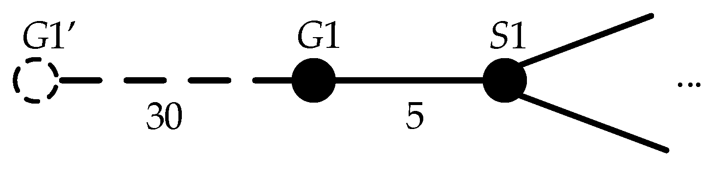
For each edge , a weight is assigned. In this paper, the restoration time (in minutes) of a transmission line or transformer is set as the weight of the corresponding edge while the start-up time (in minutes) of a generating unit is regarded as the weight of the corresponding virtual edge. In general, weather conditions, geographical locations and the operation of dispatchers effect the restoration time of a branch. The “most likely” restoration time of a branch is employed as its restoration time [24]. The start-up time depends on the inherent characteristics of a generating unit and can be obtained from its design document. Figure 2 shows a portion of a graph with weights. A transmission line is connected between buses G1 and S1. It requires 5 min to restore the transmission line, so the weight of line is set to be 5. A generating unit locates at bus G1. A virtual bus G1’ is used to represent the generating unit. The start-up time of the unit is 30 min. Thus, the weight of virtual edge is set to be 30.
3.2.2. The skeleton network Based on Minimum Spanning Tree
Let denote a spanning tree of , where . If the total weight of , defined by Equation (6), is the minimum among all spanning trees of , then is regarded as a minimum spanning tree (MST) of [41]. In this paper, the MST is used as the skeleton network of the power system. The represents the set of edges in the skeleton network. equals the restoration or start-up time for the corresponding component. Therefore, the equals to the total restoration time of actual lines and the start-up time of generating units in the skeleton network.
Theorem 1.
Suppose is a MST of . Let denote a subtree of , where and . is an induced subgraph of , whose vertex set is , the same as , and whose edge set consists of all edges of which have both ends in . Then, is a MST of .
Proof of Theorem 1.
Suppose for contradiction that is not a MST of . Let be a MST of , so . Construct a tree , where . It can be verified that is a spanning tree of and , so is not a MST of , and we have a contradiction. □
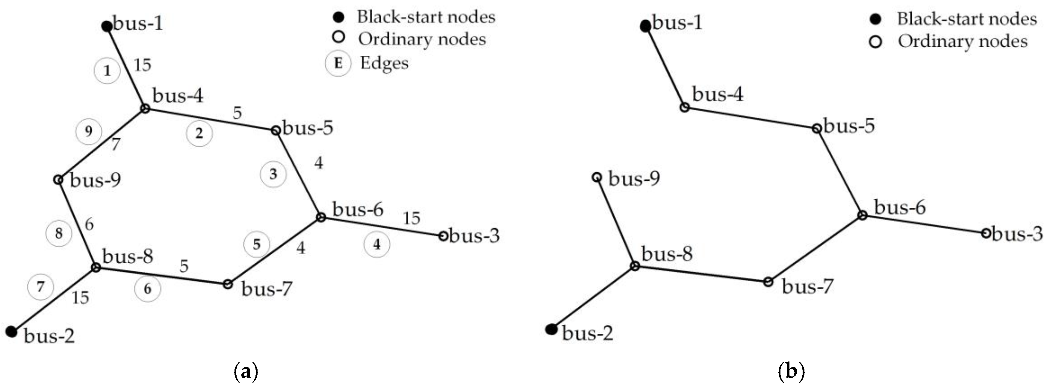
Based on Theorem 1, the skeleton network is used for sectionalizing a power system and estimating the restoration time of subsystems, considering the start-up time of generating units and the restoration time of branches. The Prim’s algorithm is a common MST method [41]. It starts from an arbitrary root vertex until the tree spans all the vertices. The minimum weight edge from the growing tree to an isolated vertex is found at each step. It is similar to the greedy algorithm as it adds an edge to the spanning tree, which contributes the minimum amount possible to the tree’s weight at each step. A skeleton network of IEEE 9-bus test system based on the Prim’s algorithm is shown in Figure 3.
In Figure 3a, the value between two buses is the edge weight. For example, the weight of edge 2 connecting bus-4 and bus-5 is 5. The algorithm adds edges 1, 2, 3, 5, 6, 8, 7 and 4 to the spanning tree in sequence. Figure 3b shows the final skeleton network of the test system.
The skeleton network is used for sectionalizing a power system for parallel restoration. The restoration time of each subsystem can be estimated according to each skeleton subnetwork. Therefore, the restoration time of subsystem is calculated as
where is the weight of edge in the skeleton network; is a binary variable. If is equal to 1, line belongs to subnetwork .
3.3. Candidate Sectionalizing Schemes Generation
In order to sectionalize a power system for parallel restoration successfully, there must be at least a black-start generating unit in each subsystem. Between any two black-start units, there is only one acyclic path on the skeleton network. Edges on the acyclic paths connecting any two black-start units can be selected as the boundary lines. These edges are named by the candidate edges (CE) for boundary lines in this paper.
Exhaustive search is used to provide all candidate sectionalizing schemes. In a scheme, if the boundary lines include CEs, the skeleton network is sectionalized into subnetworks, namely subsystems. The number of CEs is generally much less than that of all edges. Therefore, the number of candidate sectionalizing schemes for constraints evaluation does not increase largely as the scale of system expands.
3.4. Constraint Evaluation
The proposed objective function is related to the edges in the graph. However, sectionalizing Equations (2)–(4) are related to the nodes. The incidence matrix, representing the relationship between nodes and edges in a graph, is used to formulate sectionalizing constraints.
3.4.1. Constraint on the Number of Subsystems
Equation (2) guarantees that there is at least one available black-start generating unit for supplying the cranking power in each subsystem. This paper defines a black-start incidence matrix as follows
where represents the relationship between black-start unit node and edge . is the number of edges and is the number of nodes of the skeleton network. If an available black-start unit locates at node which is one terminal of edge , the is equal to 1. For example, the black-start units locate at bus-1 and bus-2 in Figure 3b. is obtained, with while other elements equal to 0. It indicates that the black-start unit at bus-1 is related to edge 1, while the black-start unit at bus-2 is related to edge 7. In subsystem , a black-start indicator index is defined as
In this paper, a black-start judgment matrix is defined as . The number of available black-start generating units in each subsystem is represented by . It is equal to the number of non-zero elements in . To meet Equation (2), all elements of the must be not less than 1. It is described as
where .
3.4.2. Minimum Output Constraint on Generating Units
The minimum active power output of a generating unit depends on the unit’s characteristic. It is not the emphasis of this paper. Dispatchable loads are used to balance the minimum output during the starting process of generating units and maintain a necessary amount of power output of each generating unit in each subsystem. This paper defines a minimum output incidence matrix as follows
If edge connects a generating unit or a dispatchable load located at bus , the is equal to 1. For example, there are generating units at buses 1, 2 and 3, and a dispatchable load at bus-9 in Figure 3b. is obtained, with while other elements equal to 0.
A minimum output judgment matrix is defined as . represents the imbalance of generating units’ minimum output and dispatchable loads (IMODL) in subsystem and is calculated by
where is the IMODL at bus . The is the component-wise logical operator “AND”. To meet Equation (3), all elements of the must be not larger than 0. It is described as
where .
3.4.3. Capacity Constraint on Generating Units
Each subsystem should have sufficient capacity to maintain a satisfactory frequency by matching generation capacity and load demand. All critical loads need to be restored before resynchronization of subsystems. Therefore, this paper defines a capacity incidence matrix :
If edge connects a generating unit or a critical load located at bus , the is equal to 1. For example, there are critical loads at bus-5 and bus-7 in Figure 3b. is obtained, with while other elements are equal to 0.
A capacity judgment matrix, defined as . , represents the imbalance of generating units’ output and restored loads (IORL) in subsystem and is calculated by
where is the imbalance of units’ output and critical loads (IOCL) at bus . To meet Equation (4), all elements of the must be not less than 0. It is described as
The proposed model contains four constraints. Equation (5) is achieved in the abstraction of a power system in Section 3.2.1. In this section, Equations (2)–(4) are reformulated by Equations (10), (13) and (16), respectively. If Equations (10), (13) and (16) are true, the corresponding constraints are satisfied and feasible solutions are achieved.
3.5. Optimal Sectionalizing Schemes
After examining all kinds of constraints, feasible sectionalizing schemes are obtained. In a scheme, the restoration time of each subsystem is estimated based on its skeleton subnetwork with consideration of the generating units’ start-up time and the branches’ restoration time. Sectionalizing schemes with the minimum SRT are the optimal solutions for parallel restoration.
For a large power system, there can be more than one optimal scheme with the same minimum SRT. One of these schemes can be selected for application according to other factors by power system dispatchers, such as the generation-load imbalance.
4. Case Studies
Simulations are performed with the IEEE 39-bus and 118-bus test systems using MATLAB R2012a on a PC with an Intel Xeon E5-2650 2.30-GHz processor and 32 GB of RAM. First, the IEEE 39-bus system is used for the illustration of the proposed method. The effectiveness of the proposed approach is verified by comparing with the method proposed in [24,26]. Second, two scenarios are considered for the IEEE 118-bus system. Scenario 1 assumes that all devices in the system are available, while the impact of faulted devices on the restoration scheme is investigated in Scenario 2.
4.1. IEEE 39-Bus Test System
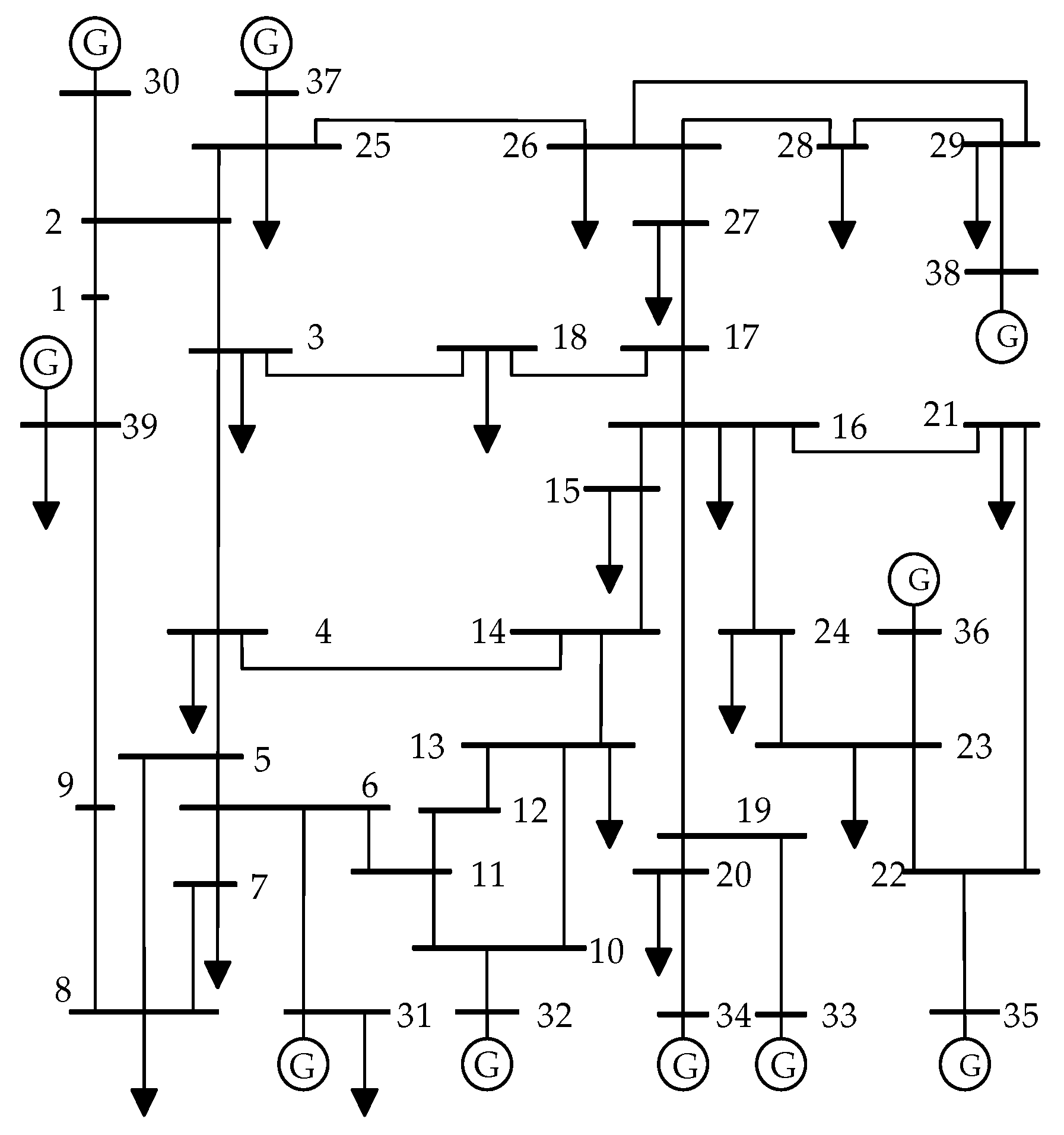
There are 10 generating units, 39 buses, 46 branches and 19 loads in the IEEE 39-bus test system, as shown in Figure 4. The system data is taken from the MATPOWER [42].
For the sake of comparison, the settings in [24] are used in this paper. The generating units at buses 30, 31 and 34 are selected as the black-start units. Therefore, the number of subsystems will not exceed three. Black-start units are usually hydropower units or gas-turbine units [43,44], which can restart without off-site power and output cranking power quickly. These types of generating units are not limited by minimum active power output. Their minimum output is usually set as 0 [30]. The lower limit of active power output of a generating unit is usually 25% of its nominal power or higher [12]. In this paper, it is set to be 30% of the nominal power. The data of units’ start-up time and branches’ restoration time are obtained from [15]. Loads at buses 7, 18, 21, 23 and 26 are defined as critical loads while other loads are treated as the dispatchable loads.
4.1.1. Construct the Skeleton Network Based on MST
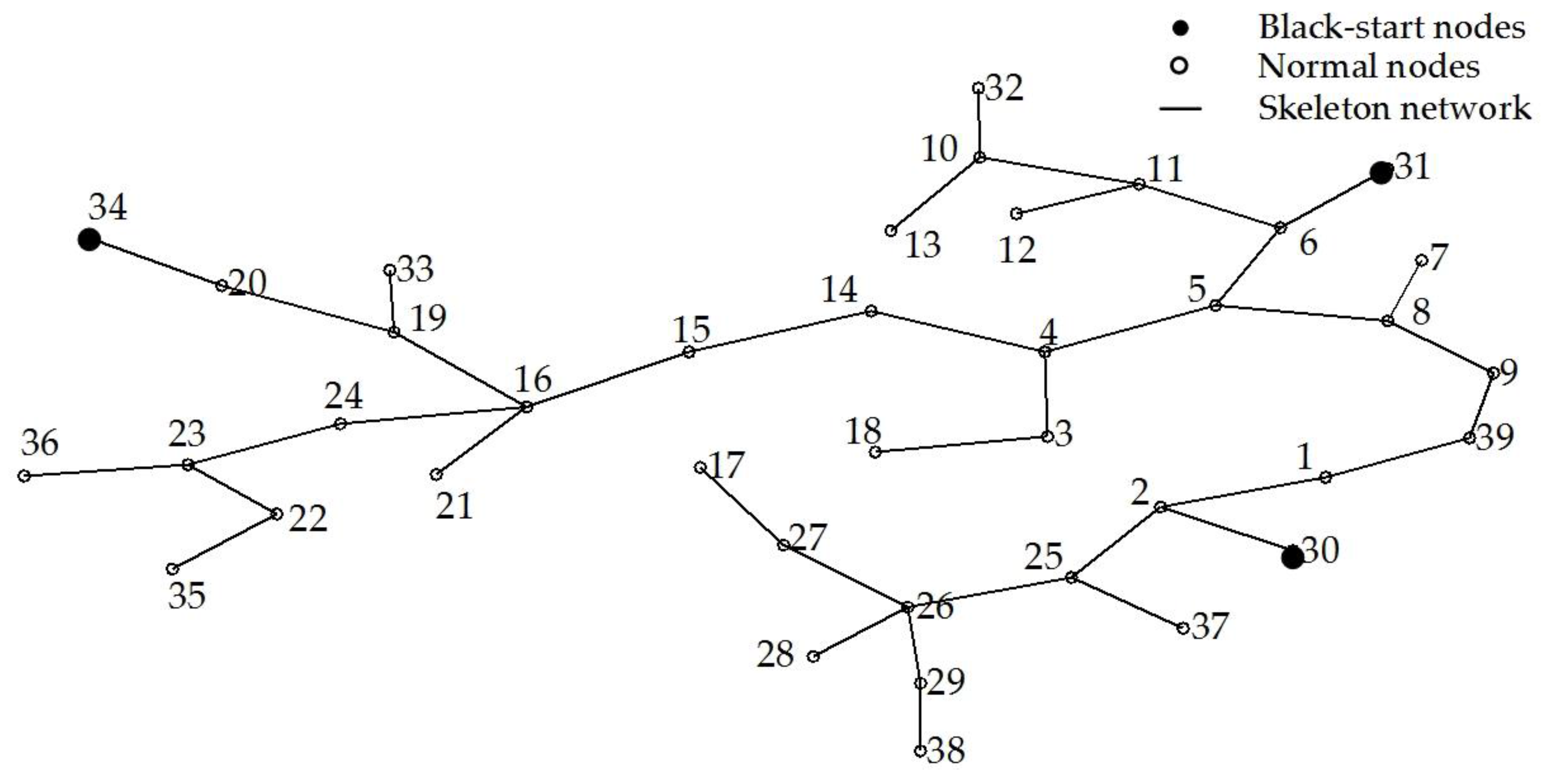
The IEEE 39-bus system is abstracted as a single-line graph containing 39 vertexes and 46 edges (virtual edges not included). The restoration time of each actual edge is set as its weight. Based on the MST, the skeleton network, including 38 edges (virtual edges not included), is constructed and presented by the solid lines in Figure 5. The dotted lines represent the edges not belong to the skeleton network. The added virtual lines, representing start-up times of generating units, are not displayed.
4.1.2. Generate Candidate Schemes
There are three paths connecting black-start units, as shown in Table 1. Some edges are the common elements in different paths. For example, the edge 15–16 belongs to both paths 2 and 3. Thus, 15 edges, 1–2, 1–39, 2–30, 4–5, 4–14, 5–6, 5–8, 6–31, 8–9, 9–39, 14–15, 15–16, 16–19, 19–20 and 20–34, are selected as the CEs of boundary lines. In this case, there are two boundary lines in a sectionalizing scheme. The candidate sectionalizing schemes’ number is by the exhaustive algorithm.
4.1.3. Evaluate Constraints
The matrices represented the IMODL and IOCL of all buses are respectively given as
And
The constraints in Section 3.4.1, Section 3.4.2 and Section 3.4.3 are examined for 105 candidate sectionalizing schemes. Seventy-six of them violate at least one of the constraints and are removed from the candidate list. For example, in the scheme with edges 1–39 and 8–9 as boundary lines, the black-start judgment matrix is . Compared with the criterion matrix , the third element of is less than 1. It means that there is no black-start unit in subsystem 3. The scheme with the edges 4–5 and 5–8 as the boundary lines is another infeasible one, which violates the minimum output constraint on generating units. The minimum output judgment matrix of this scheme is . Compared with the matrix , the second element of is larger than 0. It means that the dispatchable loads are not enough to balance the units’ minimum output during the start-up of generating units in subsystem 2. Finally, 29 schemes satisfy all sectionalizing constraints.
4.1.4. Determine the Optimal Sectionalizing Scheme
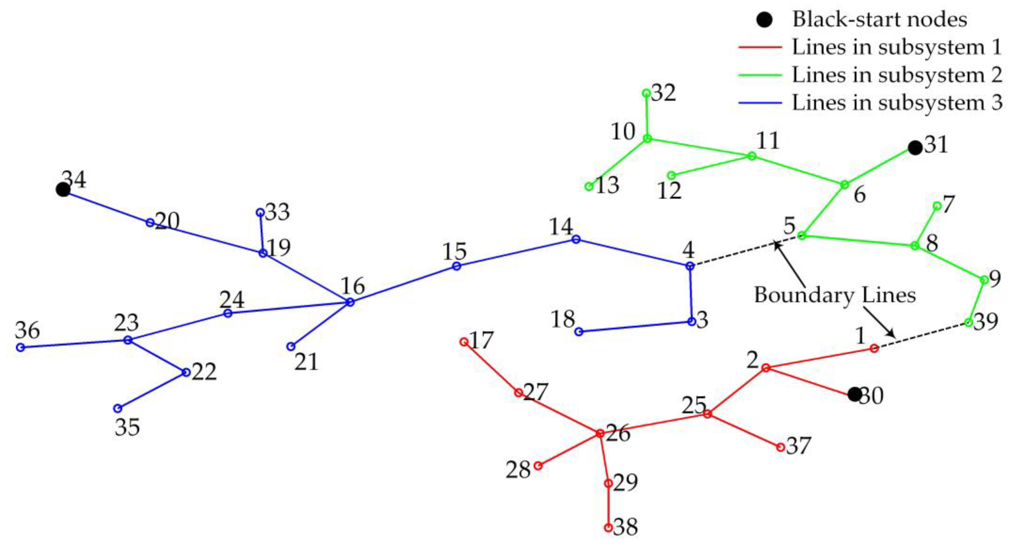
The SRT of the sectionalizing scheme with the edges 1–39 and 4–5 as the boundary lines is the minimum of all feasible schemes. Therefore, it is the optimal sectionalizing scheme and shown in Figure 6. The detail result of this scheme is given in Table 2.
Table 2 shows that the capacity margin of generating units in each subsystem is sufficient to restore interrupted loads and maintain the frequency at an acceptable level. The dispatchable loads in all subsystems are abundant for the restart of generating units.
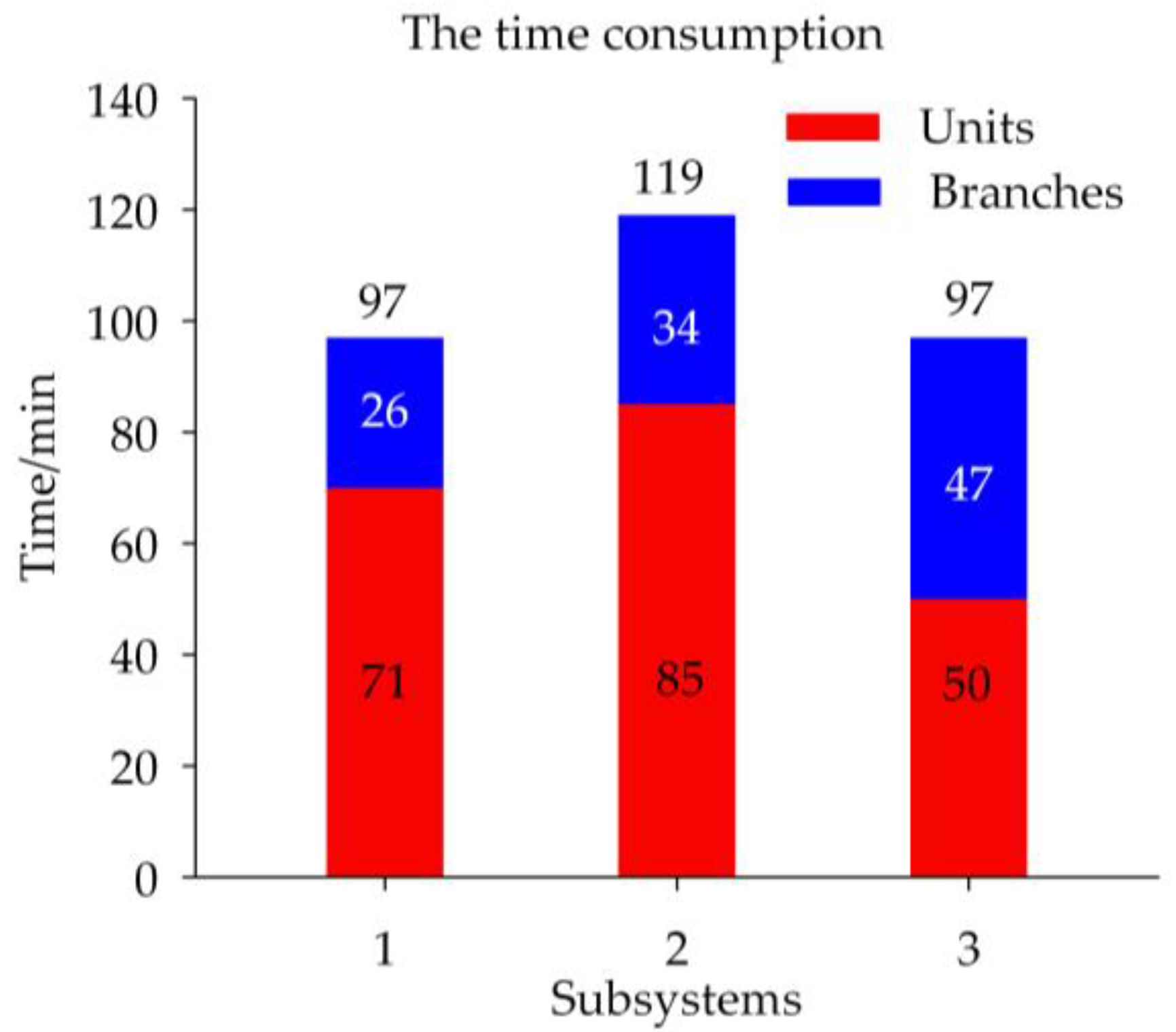
In the scheme, the restoration process of subsystem 2 is the slowest among all subsystems. Therefore, the SRT, which depends on the restoration time of subsystem 2, is 119 min. In subsystem 2, the restoration of generating units G32 and G39 takes 85 min, which is more than 70% of the restoration time of this subsystem. Although the restoration time of subsystem 1 is the same as that of subsystem 3, the scale of subsystem 1 is smaller than that of subsystem 3. The reason is that it takes longer time to restart generating units of subsystem 1 (G37 and G38) than subsystem 3 (G33, G35 and G36). The restoration time consumption of subsystems is shown in Figure 7. It indicates that the start-up time of generating units is also an important factor for sectionalization of parallel restoration.
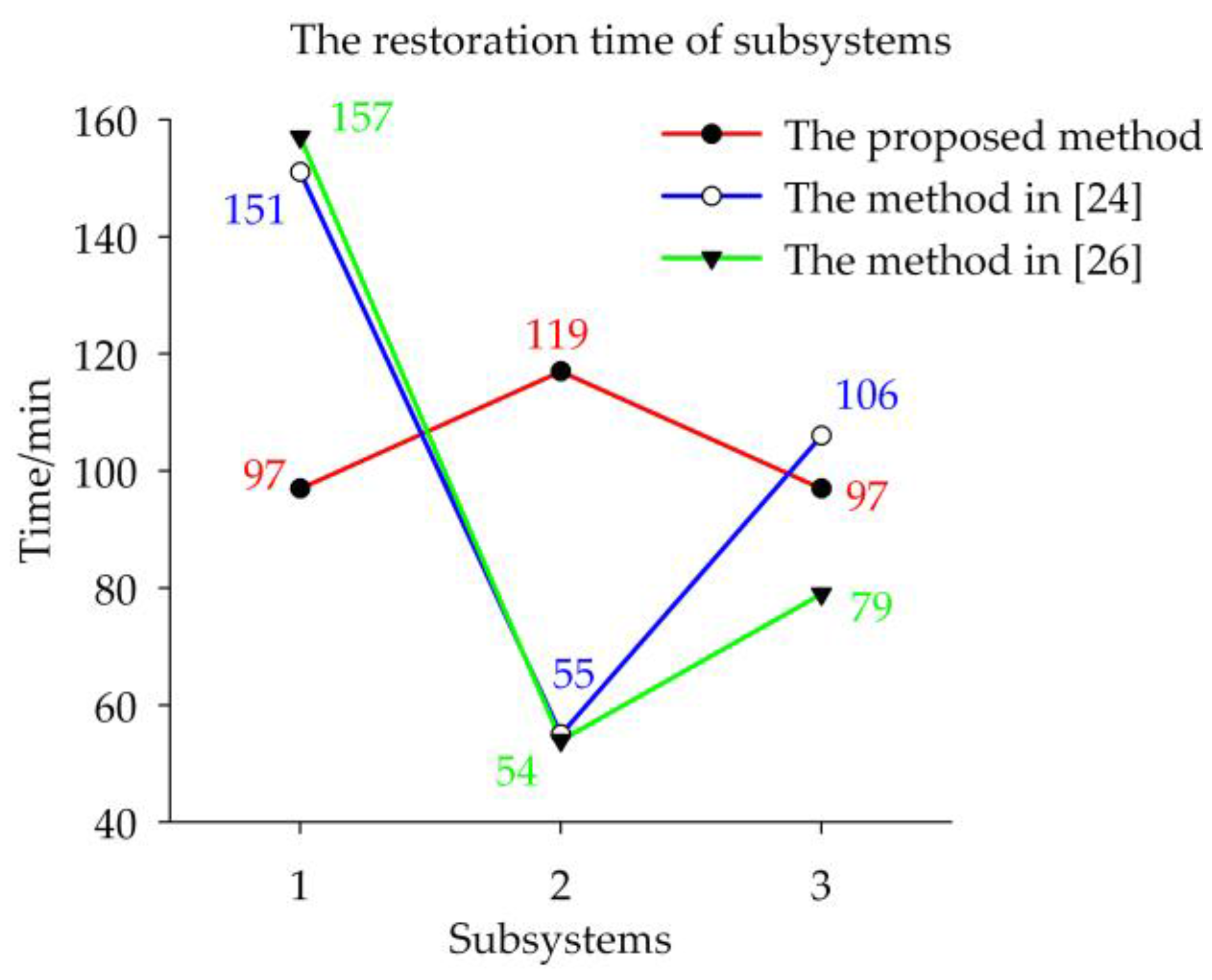
To illustrate the effectiveness of the proposed method, the results obtained by the proposed method are compared with those obtained by the methods in [24,26], as shown in Table 3 and Figure 8.
The SRT of sectionalizing scheme obtained by the method in [24] is 151 min, which depends on subsystem 1. The restoration process in subsystem 1 is also the slowest in the sectionalizing result determined by the method in [26]. The SRT of sectionalizing scheme by the method in [26] is 157 min. Table 3 and Figure 7 show that the SRT of the optimal scheme provided by the proposed method is shorter than that of the methods in [24] or [26].
The method in [26] is based on the Girvan–Newman (GN) algorithm of complex network theory. It sectionalizes a power system only based on the topology of a power system. Any factor on restoration time is not considered. The method in [24] divides a power system considering the minimum time of each unit for getting cranking power from black-start units, which represents the relationship among non-black-start units and black-start units. Therefore, the SRT by the method in [24] is shorter, as shown in the Figure 8. Nevertheless, the method in [24] ignores the time consumption on starting the generating units and energizing the transmission network. To evaluate the restoration time of subsystems, the proposed method synthesizes the restart of generating units and the restoration of skeleton transmission network. Therefore, the SRT estimation by the proposed method is more accurate.
4.2. IEEE 118-Bus Test System
There are 54 units, 118 buses, 186 branches and 98 loads in the IEEE 118-bus test system. The system data are taken from MATPOWER. There are three black-start units, located at buses 31, 54 and 87. The minimum active power output of each non-black-start unit is also set as 30%. Sixteen critical loads are defined. The other 82 loads are dispatchable loads. The restoration time of each transformer is set as 15 min because of its restoration complexity. The restoration time of each transmission line is a random value from 3 to 12 min. The start-up time of each non-black-start unit is set between 20 and 55 min. Two scenarios are studied: Scenario 1 assumes that all devices are available for restoration; and Scenario 2 valuates the impacts of faulted devices on restoration scheme by assuming that some devices of system are not available for restoration after a blackout.
4.2.1. Scenario 1: All Devices Are Available for Restoration
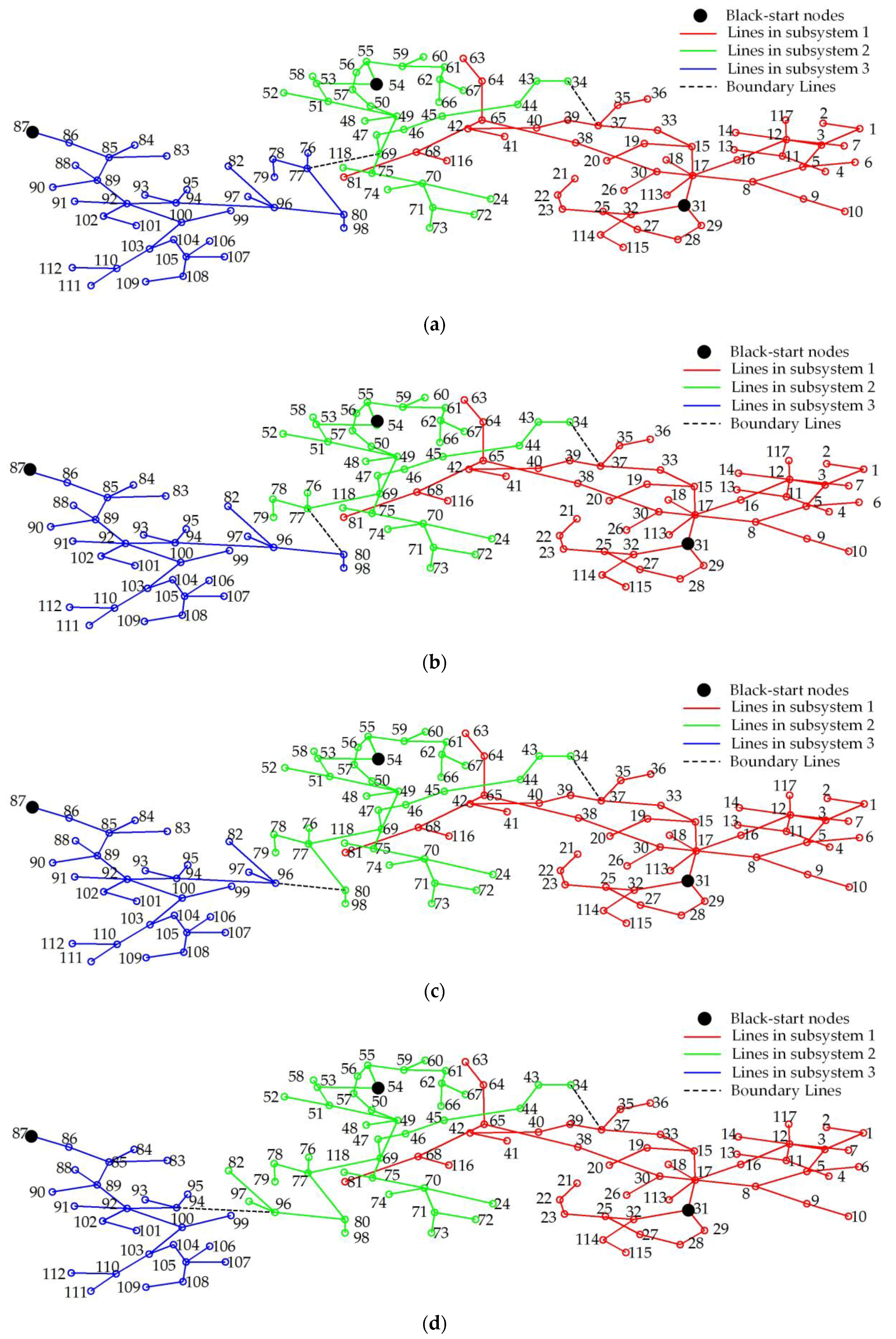
Suppose that all generating units, buses, transformers, transmission lines and loads are available for restoration in this scenario. Hence, every device of the system is used to form a graph. The skeleton network with 117 edges is constructed based on the MST. After executing this sectionalizing procedure, four optimal schemes are identified, which sectionalize the test system into three subsystems, shown in Figure 9. Their SRTs are 1004 min.
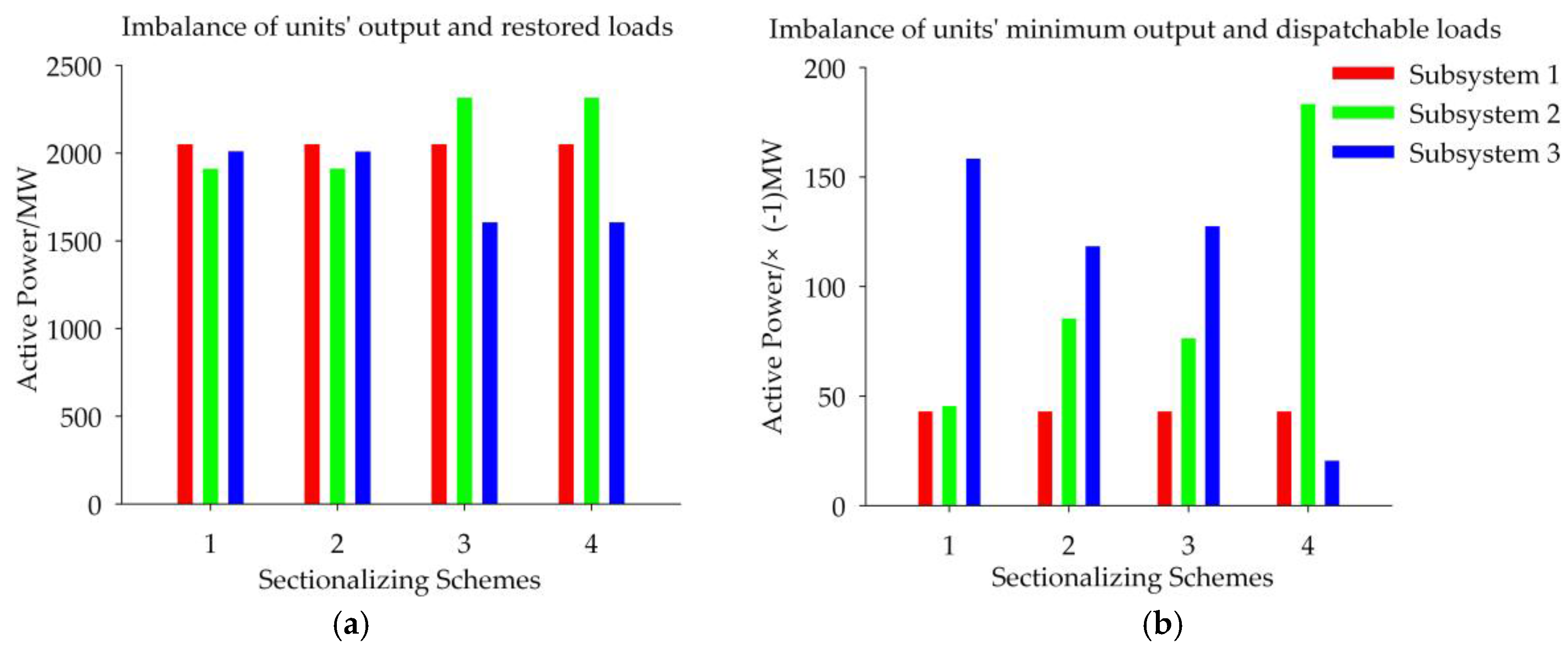
The IORL and the IMODL are two important factors for guiding operators to select a scheme for application from the list of optimal schemes. These two factors of the four schemes are shown in Figure 10.
For the imbalance of units’ output and restored loads, the schemes 1 and 2 are well-balanced. For the imbalance of units’ minimum output and dispatchable loads, the schemes 2 and 3 are well-balanced. Making comprehensive consideration of these two imbalance factors, the scheme 2 is more likely to be adopted. This scheme sectionalizes this system by edges 34–37 and 77–80 and its result is shown in Table 4.
Table 4 shows that the capacity margin of generating units in each subsystem is enough to restore interrupted loads and maintain the frequency in a reasonable profile. The imbalance of unit’s minimum output and dispatchable loads in subsystem 1 is smaller than that of subsystem 2 or 3. Therefore, the application of dispatchable loads should be paid more attention during the start-up process of generating units in subsystem 1.
4.2.2. Scenario 2: Sectionalizing with Unavailable Devices
It is assumed that some devices are not available after the blackout. It has an influence on the sectionalizing result. For example, if a faulted line needs too much time to be repaired, it should not be used as the boundary lines of subsystems. The unavailable devices in this scenario are as follows:
- The non-black-start unit at bus 72;
- The line 34–37; and
- The loads at buses 1 and 2.
After executing the proposed procedure, a topology graph is formed without the edge 34–37, which is a boundary line in Scenario 1. The 72nd elements of and are set as 0 since the generating unit at bus 72 is not able to supply power during the restoration. There are four optimal schemes, sectionalizing this system into three subsystems. Their SRTs are 1071 min. By evaluating IORL and IMODL, the sectionalizing scheme with edges 45–46 and 77–80 as the boundary lines is selected. The indexes of each subsystem are given in Table 5.
Table 5 shows that the imbalance of units’ minimum output and dispatchable loads in subsystem 1 is smaller than that in subsystems 2 or 3. Therefore, more attention should be paid to the start-up process of generating units in subsystem 1. All subsystems have the sufficient generation capacity to pick up interrupted loads.
The main difference between scenarios 1 and 2 is the boundary line between the subsystems 1 and 2. As the edge 34–37 is unavailable for restoration, it cannot be a boundary line in Scenario 2. Meanwhile, comparing with the Scenario 1, buses 43, 44 and 45 are moved from subsystem 2 to subsystem 1 in Scenario 2. This is because the dispatchable loads at buses 1 and 2 are not available in Scenario 2. The total capacity of the lost dispatchable loads is 71 MW. It is concluded from the Table 4 that the dispatchable loads are not enough to balance the minimum output of units. In order to meet the minimum output constraint on units, dispatchable loads at buses 43, 44 and 45 are merged into subsystem 1. Since the generation capacity margin of each subsystem is fully plenty, the lack of generating unit at bus 72 does not affect the sectionalizing result.
4.3. Discussions
4.3.1. About the Objective Function
The subsystem with the slowest restoration process consumes the maximum restoration time among all subsystems. In this paper, the system restoration time (SRT) is defined by the maximum restoration time of the subsystem. The objective function is to minimize the SRT. There is a kind of sectionalizing methods with the objective to minimize difference in restoration time of subsystems, such as [21]. Their solutions are to minimize the difference between the maximum and the minimum restoration time of subsystems. To shorten the maximum restoration time of subsystem can increase the restoration time of other subsystems. It also helps reduce the difference in restoration time of subsystems. Thus, the objectives have similar effects.
The objective to minimize the difference in restoration time of subsystems usually generates a single sectionalizing scheme. However, any circumstance may render the unique scheme unpractical for preparing parallel restoration plans [23]. Thus, a shortlist of sectionalizing schemes should be prepared for a large power system. The objective in this paper can provide multiple schemes for dispatchers. For instance, four sectionalizing schemes of IEEE 118-bus test system are obtained in Section 4.2.1. The dispatchers can select one for application based on their knowledge and the specific nature of the restoration, which is more flexible for actual large systems.
4.3.2. Remarks on Computational Time
The proposed method includes four steps. The first step uses the Prim’s algorithm to construct the skeleton network. Its time complexity is , where denotes the number of nodes [41]. The second step is to generate candidate sectionalizing schemes by exhaustive algorithm with a complexity of , where is the number of CEs for boundary lines and the is the number of subsystems. Since the number of subsystems will not be too large in practice, the number of candidate schemes will not increase with the scale of power system expanding significantly. To evaluate all kinds of constraints, the multiplication on the decision matrix of size and the modified incidence matrixes of size has a complexity of in the third step, where is the number of edges of the skeleton network. The restoration time of each subsystem is calculated by the multiplication on the decision matrix and the time matrix of size in the last step. It takes to achieve solutions. Thus, the time complexity of this method is . Since is much larger than and is nearly equal to , the total complexity of the proposed method is . For the IEEE 118-bus test system, the computational time for each step is as follows:
- The first step, i.e., constructing the skeleton network, consumes 0.259 s.
- The second step, i.e., generating candidate sectionalizing schemes, consumes 0.157 s.
- The third step, i.e., evaluating constraints, consumes 8.142 min. Parallel computation techniques can be used to reduce the computational time of this step.
- The last step, i.e., selecting optimal or near optimal schemes, consumes 0.02 s.
4.3.3. Hybrid Renewable Energy System for Restoration
With the development of renewable generation and microgrids, high-density hybrid renewable energies are embedded in power systems. The optimal operation and control, reconfiguration, voltage imbalance, and fault analysis of hybrid renewable energy systems (HRES) have been studied in [45,46,47,48,49,50,51,52]. Besides, HRES such as photovoltaic-energy storage systems (PV-ESS) and microgrid distribution systems can be used as black-start energy. Based on them, new restoration strategies are proposed in [53,54]. The power flow analysis and voltage imbalance evaluation for HRES [11,50,51,52,53,54,55] is still a challenge in power system restoration. The integration of HRES models into the proposed method will be studied in the future.
5. Conclusions
We have proposed a novel sectionalizing method for power system parallel restoration based on graph theory, considering the start-up time of generating units and the restoration time of branches. A new constraint on dispatchable loads for balancing the minimum output of generating units is incorporated. The proposed method provides sectionalizing schemes with the minimum SRT. Simulations on the IEEE 39 and 118-bus test systems are performed to evaluate the effectiveness of the proposed method. The case studies indicates that the proposed method is effective for shortening the duration of power outage and improving the security and reliability of power systems. The detailed findings include:
- (1)
- The proposed method seeks to minimize the SRT, which helps balance the restoration time of subsystems. It can provide multiple schemes so that dispatchers can choose one for application according to actual requirement.
- (2)
- The proposed method is based on the MST. It identifies the candidate boundary lines according to the skeleton network. It can reduce the search space for solution and shorten the computational time for large-scale power systems.
- (3)
- The SRT depends on the start-up time of generating units and the restoration time of branches. In particular, the start-up time of generating units is an important factor for sectionalization. Therefore, it cannot be ignored for the estimating the restoration time.
- (4)
- The proposed method is suitable for power systems under various conditions, including the conditions when some components are damaged. The case study results indicate that faulted devices may have negative effects on the SRT.
Acknowledgments
The authors would like to appreciate the Project Supported by the National Key R&D Program of China, Grant No. 2016YFB0900600, and the Fundamental Research Funds for the Central Universities, Grant No. 2015YJS158.
Author Contributions
Changcheng Li is responsible of designing the proposed method and performing the simulation tests; this work was performed under the supervisory of Jinghan He and Pei Zhang; Yin Xu provided advice for this method and revise this paper with regular feedback; and all the authors have read and approved the final manuscript.
Conflicts of Interest
The authors declare no conflict of interest.
Nomenclature
| graph representing a power system | |
| minimum spanning tree, i.e., skeleton network | |
| set of nodes in graph G | |
| set of edges in graph G | |
| set of edges in skeleton network T | |
| total weight of edges | |
| number of subsystems | |
| index of subsystems | |
| restoration time of subsystem | |
| number of nodes in a power system | |
| number of nodes in subsystem | |
| number of black-start generating units | |
| index of nodes | |
| number of edges in a power system | |
| index of edges in a power system | |
| weight of edge in a power system | |
| number of edges in the skeleton network | |
| index of edges in the skeleton network | |
| weight of edge in the skeleton network | |
| decision variable of edge in the skeleton network. If edge belongs to subsystem , ; otherwise, | |
| number of candidate edges for boundary lines | |
| total active power capacity of the generating units at bus in subsystem | |
| total minimum output of the generating units at bus in subsystem | |
| imbalance of generating units’ minimum output and dispatchable loads at bus | |
| imbalance of generating units’ output and critical loads at bus | |
| total active power demand of the critical loads at bus in subsystem | |
| total active power demand of the dispatchable loads at bus in subsystem | |
| set of faulted devices | |
| set of devices available for restoration | |
| black-start incidence matrix | |
| -element of . If an available black-start unit locates at node which is one terminal of edge , the ; otherwise, | |
| black-start judgment matrix for the constraint on the number of subsystems | |
| black-start indicator index for subsystem | |
| number of available black-start generating units in subsystem | |
| minimum output incidence matrix | |
| -element of . If edge connects a generating unit or a dispatchable load located at bus , the ; otherwise, | |
| minimum output judgment matrix for the minimum output constraint on generating units | |
| imbalance of generating units’ minimum output and dispatchable loads in subsystem | |
| capacity incidence matrix | |
| -element of . If edge connects a generating unit or a critical load located at bus , the ; otherwise, | |
| capacity judgment matrix for the capacity constraint on generating units | |
| imbalance of generating units’ output and restored loads in subsystem | |
| MST | minimum spanning tree |
| SRT | the system restoration time |
| CE | the candidate edge |
| IMODL | the imbalance of generating units’ minimum output and dispatchable loads |
| IOCL | the imbalance of units’ output and critical loads |
| IORL | the imbalance of generating units’ output and restored loads |
References
- Andersson, G.; Donalek, P.; Farmer, R.; Hatziargyriou, N. Causes of the 2003 major grid blackouts in north america and europe, and recommended means to improve system dynamic performance. IEEE Trans. Power Syst. 2005, 20, 1922–1928. [Google Scholar] [CrossRef]
- Li, C.; Sun, Y.; Chen, X. Analysis of the blackout in Europe on 4 November 2006. In Proceedings of the 2007 International Power Engineering Conference, Singapore, Singapore, 3–6 December 2007; pp. 939–944. [Google Scholar]
- Ministry of Indian Power. Report of the Enquiry Committee on Grid Disturbance in Northern Region on 30th July 2012 and in Northern, Eastern & North-Eastern Region on 31st July 2012; Enquiry Committee of Ministry of Indian Power: New Delhi, India, 2012.
- Project Group Turkey. Report on Blackout in Turkey on 31st March 2015; TEIAS and ENTSO-E: Brussels, Belgium, 2015. [Google Scholar]
- Mehdi, G.; Neng, F.; Jianhui, W. Two-stage stochastic optimal islanding operations under severe multiple contingencies in power grids. Electr. Power Syst. Res. 2014, 114, 68–77. [Google Scholar]
- Sarwat, A.I.; Amini, M.; Domijan, A.; Damnjanovic, A.; Kaleem, F. Weather-based interruption prediction in the smart grid utilizing chronological data. J. Mod. Power Syst. Clean Energy 2016, 5, 308–315. [Google Scholar] [CrossRef]
- Boroojeni, K.G.; Amini, M.H.; Iyengar, S.S. Smart Grids: Security and Privacy Issues; Springer: Cham, Switzerland, 2017. [Google Scholar]
- Sarwat, A.I.; Domijan, A.; Amini, M.H.; Damnjanovic, A.; Moghadasi, A. Smart Grid reliability assessment utilizing Boolean Driven Markov Process and variable weather conditions. In Proceedings of the 2015 North American Power Symposium (NAPS), Charlotte, NC, USA, 4–6 October 2015. [Google Scholar]
- Golari, M.; Fan, N.; Wang, J. Large-scale stochastic power grid islanding operations by line switching and controlled load shedding. Energy Syst. 2016, 7, 1–21. [Google Scholar] [CrossRef]
- Liu, Y.T.; Fan, R.; Terzija, V. Power system restoration: a literature review from 2006 to 2016. J. Mod. Power Syst. Clean Energy 2016, 4, 1–10. [Google Scholar] [CrossRef]
- Pesoti, P.M.; Lorenci, E.D.; Souza, A.Z.D.; Lo, K.; Lopes, B.L. Robustness area technique developing guidelines for power system restoration. Energies 2017, 10, 99. [Google Scholar] [CrossRef]
- Adibi, M.; Clelland, P.; Fink, L.; Happ, H. Power system restoration—A task force report. IEEE Trans. Power Syst. 1987, 2, 271–277. [Google Scholar] [CrossRef]
- Fink, L.H.; Liou, K.L.; Liu, C.C. From generic restoration actions to specific restoration strategies. IEEE Trans. Power Syst. 1995, 10, 745–752. [Google Scholar] [CrossRef]
- Sun, W.; Liu, C.C.; Zhang, L. Optimal generator start-up strategy for bulk power system restoration. IEEE Trans. Power Syst. 2011, 26, 1357–1366. [Google Scholar] [CrossRef]
- Zhang, C.; Lin, Z.; Wen, F.; Ledwich, G. Two-stage power network reconfiguration strategy considering node importance and restored generation capacity. IET Gener. Trans. Distrib. 2014, 8, 91–103. [Google Scholar] [CrossRef]
- Liu, W.; Lin, Z.; Wen, F.; Ledwich, G. A wide area monitoring system based load restoration method. IEEE Trans. Power Syst. 2013, 28, 2025–2034. [Google Scholar] [CrossRef]
- System Operations Division. PJM Manual 36: System Restoration; PJM: Audubon, PA, USA, 2010. [Google Scholar]
- National Grid Electricity Transmission. The Grid Code; National Grid Electricity Transmission: Warwick, UK, 2016.
- Chen, T.; Feng, L.; Liu, X.; Zhang, L. Comparison study on restoration strategies of Chongqing power grid. In Proceedings of the 5th International Conference on Electric Utility Deregulation and Restructuring and Power Technologies, Changsha, China, 26–29 November 2015; pp. 2425–2430. [Google Scholar]
- Wang, C.; Vittal, V.; Sun, K. OBDD-based sectionalizing strategies for parallel power system restoration. IEEE Trans. Power Syst. 2011, 26, 1426–1433. [Google Scholar] [CrossRef]
- Afrakhte, H.; Haghifam, M.R. Optimal islands determination in power system restoration. Iran. J. Sci. Technol. Trans. B Eng. 2009, 33, 463–476. [Google Scholar]
- Liang, H.P.; Gu, X.P.; Zhao, D. Optimization of system partitioning schemes for power system black-start restoration based on genetic algorithms. In Proceedings of the 2010 Asia-Pacific Power and Energy Engineering Conference, Chengdu, China, 28–31 March 2010; pp. 1–4. [Google Scholar]
- Quirós-Tortós, J.; Panteli, M.; Wall, P.; Terzija, V. Sectionalising methodology for parallel system restoration based on graph theory. IET Gener. Trans. Distrib. 2015, 9, 1216–1225. [Google Scholar]
- Sun, L.; Zhang, C.; Lin, Z.; Wen, F. Network partitioning strategy for parallel power system restoration. IET Gener. Trans. Distrib. 2016, 10, 1883–1892. [Google Scholar] [CrossRef]
- Sarmadi, S.A.N.; Dobakhshari, A.S.; Azizi, S.; Ranjbar, A.M. A sectionalizing method in power system restoration based on WAMS. IEEE Trans. Smart Grid 2011, 2, 190–197. [Google Scholar] [CrossRef]
- Lin, Z.Z.; Wen, F.S.; Chung, C.Y.; Wong, K.P. Division algorithm and interconnection strategy of restoration subsystems based on complex network theory. IET Gener. Trans. Distrib. 2011, 5, 674–683. [Google Scholar] [CrossRef]
- Quiros-Tortos, J.; Terzija, V. A Graph Theory Based New Approach for power system restoration. In Proceedings of the IEEE-PES Powertech Grenoble Conference, Grenoble, France, 16–20 June 2013; pp. 1–6. [Google Scholar]
- Quiros, J.; Wall, P.; Ding, L.; Terzija, V. Determination of sectionalising strategies for parallel power system restoration: A spectral clustering-based methodology. Electr. Power Syst. Res. 2014, 116, 381–390. [Google Scholar] [CrossRef]
- Adibi, M.M.; Milanicz, D.P. Estimating restoration duration. IEEE Tran. Power Syst. 1999, 14, 1493–1498. [Google Scholar] [CrossRef]
- Hou, Y.; Liu, C.C.; Sun, K.; Zhang, P. Computation of milestones for decision support during system restoration. IEEE Tran. Power Syst. 2011, 26, 1399–1409. [Google Scholar] [CrossRef]
- Mishra, R.K.; Swarup, K.S. Power system restoration in smart grid environment. In Proceedings of the 2014 Eighteenth National Power Systems Conference (NPSC), Guwahati, India, 18–20 December 2014; pp. 1–6. [Google Scholar]
- Farhad, K.; Mohammadhadi, A.; Siamak, S. Demand response program in smart grid using supply function bidding mechanism. IEEE Tran. Smart Grid 2016, 7, 1277–1284. [Google Scholar]
- Gellings, C.W.; Chamberlin, J.H. Demand-side management. In Energy Efficiency and Renewable Energy Handbook, 2nd ed.; Goswami, D.Y., Kreith, F., Eds.; CPC Press: Boca Raton, FL, USA, 2016; Chapter 15; pp. 289–310. [Google Scholar]
- Stefanov, A.; Liu, C.C.; Sforna, M.; Eremia, M. Decision support for restoration of interconnected power systems using tie lines. IET Gener. Trans. Distrib. 2015, 9, 1006–1018. [Google Scholar] [CrossRef]
- Shahidehpour, S.M.; Yamin, H.Y. A technique for the standing phase-angle reduction in power system restoration. Electr. Power Compon. Syst. 2004, 33, 277–286. [Google Scholar] [CrossRef]
- Ye, H.; Liu, Y. A new method for standing phase angle reduction in system restoration by incorporating load pickup as a control means. Int. J. Electr. Power Energy Syst. 2013, 53, 664–674. [Google Scholar] [CrossRef]
- Zhu, J.Z. Optimization of Power System Operation, 2nd ed.; Wiley-IEEE Press: Piscataway, NJ, USA, 2015; pp. 91–92. [Google Scholar]
- Mello, F.P.D.; Westcott, J.C. Steam plant startup and control in system restoration. IEEE Tran. Power Syst. 1994, 9, 93–101. [Google Scholar] [CrossRef]
- Adibi, M.M.; Fink, L.H. Overcoming restoration challenges associated with major power system disturbances—Restoration from cascading failures. IEEE Power Energy Mag. 2006, 4, 68–77. [Google Scholar] [CrossRef]
- Adibi, M.M.; Borkoski, J.N.; Kafka, R.J.; Volkmann, T.L. Frequency response of prime movers during restoration. IEEE Tran. Power Syst. 1999, 14, 751–756. [Google Scholar] [CrossRef]
- Cormen, T.H.; Leiserson, C.E.; Rivst, R.L.; Stein, C. Introduction to Algorithms, 3rd ed.; The MIT Press: Cambridge, MA, USA, 2009; pp. 624–642. [Google Scholar]
- Zimmerman, R.D.; Murillo-Sanchez, C.E.; Thomas, R.J. MATPOWER: Steady-state operations, planning, and analysis tools for power systems research and education. IEEE Tran. Power Syst. 2011, 26, 12–19. [Google Scholar] [CrossRef]
- Feltes, J.W.; Grande-Moran, C. Black start studies for system restoration. In Proceedings of the 2008 IEEE Power and Energy Society General Meeting—Conversion and Delivery of Electrical Energy in the 21st Century, Pittsburgh, PA, USA, 20–24 July 2008; pp. 1–8. [Google Scholar]
- Zeng, K.; Wen, J.; Ma, L.; Cheng, S.; Lu, E.; Wang, N. Fast cut back thermal power plant load rejection and black start field test analysis. Energies 2014, 7, 2740–2760. [Google Scholar] [CrossRef]
- Ou, T. Ground fault current analysis with a direct building algorithm for microgrid distribution. Int. J. Electr. Power Energy Syst. 2013, 53, 867–875. [Google Scholar] [CrossRef]
- Ou, T.; Su, W.; Liu, X.; Huang, S.; Tai, T. A modified bird-mating optimization with hill-climbing for connection decisions of transformers. Energies 2016, 9, 671. [Google Scholar] [CrossRef]
- Ou, T.; Lu, K.; Huang, C. Improvement of transient stability in a hybrid power multi-system using a designed NIDC (Novel Intelligent Damping Controller). Energies 2017, 10, 488. [Google Scholar] [CrossRef]
- Ou, T.; Hong, C. Dynamic operation and control of microgrid hybrid power systems. Energy 2014, 66, 314–323. [Google Scholar] [CrossRef]
- Hong, C.; Ou, T.; Lu, K. Development of intelligent MPPT (maximum power point tracking) control for a grid-connected hybrid power generation system. Energy 2013, 50, 270–279. [Google Scholar] [CrossRef]
- Ou, T.; Lin, W.; Huang, C.; Cheng, F. A hybrid programming for distribution reconfiguration of dc microgrid. In Proceedings of the 2009 IEEE PES/IAS Conference on Sustainable Alternative Energy (SAE), Valencia, Spain, 28–30 September 2009; pp. 1–7. [Google Scholar]
- Ou, T. A novel unsymmetrical faults analysis for microgrid distribution systems. Int. J. Electr. Power Energy Syst. 2012, 43, 1017–1024. [Google Scholar] [CrossRef]
- Lin, W.; Ou, T. Unbalanced distribution network fault analysis with hybrid compensation. IET Gener. Trans. Distrib. 2011, 5, 92–100. [Google Scholar] [CrossRef]
- Xu, Z.; Yang, P.; Zeng, Z.; Peng, J.; Zhao, Z. Black start strategy for PV-ESS multi-microgrids with three-phase/single-phase architecture. Energies 2016, 9, 372. [Google Scholar] [CrossRef]
- Jiang, Y.; Liu, C.; Xu, Y. Smart Distribution Systems. Energies 2016, 9, 297. [Google Scholar] [CrossRef]
- Li, H.; Abinet, T.E.; Zhang, J.; Zheng, D. Optimal energy management for industrial microgrids with high-penetration renewables. Prot. Control Mod. Power Syst. 2017, 2, 12. [Google Scholar] [CrossRef]
Figure 1.
The flow diagram of the proposed method.

Figure 2.
A weighted graph representing a power system.

Figure 3.
(a) The graph of IEEE 9-bus test system; and (b) the skeleton network.

Figure 4.
The IEEE New England 39-bus test system.

Figure 5.
The skeleton network of IEEE 39-bus test system.

Figure 6.
The optimal sectionalizing scheme of IEEE 39-bus test system.

Figure 7.
The restoration time consumption.

Figure 8.
The restoration time of subsystems using different methods.

Figure 9.
Optimal sectionalizing schemes in Scenario 1: (a) Scheme 1; (b) Scheme 2; (c) Scheme 3; and (d) Scheme 4.
Figure 9.
Optimal sectionalizing schemes in Scenario 1: (a) Scheme 1; (b) Scheme 2; (c) Scheme 3; and (d) Scheme 4.

Figure 10.
Comparison on: (a) IORL; and (b) IMODL of the candidate sectionalizing schemes.


Table 1.
The transmission paths connecting all black-start generating units.
| Index of Path | The Pair of Black-Start Units | Edges on the Path |
|---|---|---|
| 1 | 30, 31 | 30–2, 2–1, 1–39, 39–9, 9–8, 8–5, 5–6, 6–31. |
| 2 | 30, 34 | 30–2, 2–1, 1–39, 39–9, 9–8, 8–5, 5–4, 4–14, 14–15, 15–16, 16–19, 19–20, 20–34. |
| 3 | 31, 34 | 31–6, 6–5, 5–4, 4–14, 14–15, 15–16, 16–19, 19–20, 20–34. |
Table 2.
The sectionalizing result of IEEE 39-bus test system.
| Subsystems | IORL/MW | IMODL/MW | Restoration Time/Min |
|---|---|---|---|
| 1 | 1901.3 | −565.8 | 97 |
| 2 | 1689.7 | −1095.2 | 119 |
| 3 | 1171.8 | −1831.9 | 97 |
| Methods | IORL of Subsystems/MW | IMODL of Subsystems/MW | SRT of Schemes/Min | ||||
|---|---|---|---|---|---|---|---|
| Sub.1 | Sub.2 | Sub.3 | Sub.1 | Sub.2 | Sub.3 | ||
| Proposed method | 1901.3 | 1689.7 | 1171.8 | −565.8 | −1095.2 | −1831.9 | 119 |
| Method in [24] | 2671.3 | 919.7 | 1171.8 | −1880.8 | −641.2 | −970.9 | 151 |
| Method in [26] | 2513.3 | 919.7 | 1329.8 | −1661.8 | −821.2 | −1009.9 | 157 |
Table 4.
The sectionalizing result in Scenario 1.
| Subsystems | IORL/MW | IMODL/MW | Restoration Time/Min |
|---|---|---|---|
| 1 (Black-start 31) | 2050 | −43 | 1004 |
| 2 (Black-start 54) | 1911.64 | −85.44 | 833 |
| 3 (Black-start 87) | 2009.4 | −118.4 | 717 |
Table 5.
The sectionalizing result in Scenario 2.
| Subsystems | IORL/MW | IMODL/MW | Restoration Time/Min |
|---|---|---|---|
| 1 (Black-start 31) | 2061 | −29 | 1071 |
| 2 (Black-start 54) | 1830.6 | −58.44 | 768 |
| 3 (Black-start 87) | 2009.4 | −118.4 | 717 |
© 2017 by the authors. Licensee MDPI, Basel, Switzerland. This article is an open access article distributed under the terms and conditions of the Creative Commons Attribution (CC BY) license (http://creativecommons.org/licenses/by/4.0/).
Share and Cite
MDPI and ACS Style
Li, C.; He, J.; Zhang, P.; Xu, Y. A Novel Sectionalizing Method for Power System Parallel Restoration Based on Minimum Spanning Tree. Energies 2017, 10, 948. https://doi.org/10.3390/en10070948
AMA Style
Li C, He J, Zhang P, Xu Y. A Novel Sectionalizing Method for Power System Parallel Restoration Based on Minimum Spanning Tree. Energies. 2017; 10(7):948. https://doi.org/10.3390/en10070948
Chicago/Turabian StyleLi, Changcheng, Jinghan He, Pei Zhang, and Yin Xu. 2017. "A Novel Sectionalizing Method for Power System Parallel Restoration Based on Minimum Spanning Tree" Energies 10, no. 7: 948. https://doi.org/10.3390/en10070948
Note that from the first issue of 2016, this journal uses article numbers instead of page numbers. See further details here.