Article

Quick Screening of Pareto-Optimal Operating Conditions for Expanding Solvent–Steam Assisted Gravity Drainage Using Hybrid Multi-Objective Optimization Approach

1
Department of Climate and Energy Systems Engineering, Division of Sustainable Systems Engineering, Ewha Womans University, 52 Ewhayeodae-gil, Daehyeon-dong, Seodaemun-gu, Seoul 03760, Korea
2
Department of Petroleum and Geosystems Engineering, The University of Texas at Austin, TX 78712, USA
3
Department of Energy and Mineral Engineering, College of Earth and Mineral Sciences, Pennsylvania State University, University Park, PA 16802, USA
*
Author to whom correspondence should be addressed.
Energies 2017, 10(7), 966; https://doi.org/10.3390/en10070966
Submission received: 20 April 2017 / Revised: 18 June 2017 / Accepted: 5 July 2017 / Published: 10 July 2017
(This article belongs to the Section L: Energy Sources)

Abstract

:
Solvent–steam mixture is a key factor in controlling the economic efficiency of the solvent-aided thermal injection process for producing bitumen in a highly viscous oil sands reservoir. This paper depicts a strategy to quickly provide trade-off operating conditions of the Expanding Solvent–Steam Assisted Gravity Drainage (ES-SAGD) process based on Pareto-optimality. Response surface models are employed to evaluate multiple ES-SAGD scenarios at low computational costs. The surrogate models play a role of objective-estimators in the multi-objective optimization that provides qualified ES-SAGD scenarios regarding bitumen recovery, steam–energy efficiency, and solvent-energy efficiency. The developed hybrid approach detects positive or negative correlations among the performance indicators of the ES-SAGD process. The derived Pareto-optimal operating conditions give flexibility in field development planning and thereby help decision makers determine the operating parameters of the ES-SAGD process based on their preferences.

1. Introduction

Steam Assisted Gravity Drainage (SAGD) is a thermal injection technique useful for producing bitumen by lowering its viscosity (typically greater than 10,000 cP under reservoir conditions) sufficiently in oil sands reservoirs [1]. One salient issue in the SAGD process is how to save the volume of steam injected into the formation while achieving high bitumen recovery [2,3,4,5]. Researchers have led to the development of a more energy-efficient version called Expanding Solvent-SAGD (ES-SAGD). The ES-SAGD process co-injects light hydrocarbon solvent with steam for enhancing the thermal injection efficiency [6,7,8,9,10,11]. Injected solvent condenses at the vapor/liquid boundary of the steam chamber and creates a diluted interface for further reducing the viscosity of heated bitumen [12]. Nasr et al. [6] showed that the steam–solvent co-injection could increase bitumen production rate while decreasing steam injection rate compared to SAGD.
Solvent–steam mixture is a critical factor for economically operating the ES-SAGD process owing to expensive solvent costs. Ardali et al. [13] provided a review of hybrid steam–solvent processes used for in-situ recovery of Canadian heavy oil, e.g., Propane-SAGD, ES-SAGD, Solvent-Aided Process (SAP), Liquid Addition to Steam to Enhance Recovery (LASER), and Steam-Alternating-Solvent (SAS). As pointed out in [13], it is still unclear for solvent-aided processes how much the solvent concentration in the injected stream is sufficient to minimize total energy loss. The excessive solvent injection might cause adverse heat transfer at the steam–solvent–bitumen interface. Thus, it is necessary to make optimization strategies that can maximize the bitumen recovery and the steam–solvent efficiency formally. Various optimization approaches have been adopted to reduce energy consumption in solvent-aided SAGD processes. Gates and Chakrabarty [14] determined the solvent fraction in the injected stream and the solvent–steam injection pressure using simulated annealing. Kam et al. [15] designed a solvent–steam injection procedure using a back-propagation neural network for the McMurray formation of the Athabasca oil sands reservoir. Edmunds et al. [16] and Peterson et al. [17] maximized net present value (NPV) per hectare of land using genetic algorithm (GA) that perturbed steam–solvent injection rates. Proxies have also been investigated to alleviate computation costs accompanied with computationally intensive thermal reservoir simulation runs. Al-Gosayir et al. [18] implemented a hybrid technique that combined GA with a response surface model.
The optimization works above have found the operating condition compromising bitumen recovery and energy efficiency due to the form of objective functions. Conventionally, most optimization approaches that the petroleum industry has adopted are based on global-objective optimization no matter what they are either gradient-based methods [19,20,21,22] or non-gradient-based methods [23,24,25,26]. Global-objective optimization scheme converts a vector of objective functions into a single global objective function, i.e., the weighted sum of individual objective function values. For a minimization problem, exploring the global optimum is to find the smallest objective-sum that depends on the weight factors determined a priori. As a result, solutions tend to evolve in the direction of minimizing the objective-sum regardless of the characteristics of each objective function [27,28,29]. For this reason, global-objective optimization approaches are inappropriate to provide diversified solutions in case individual objective functions conflict with each other.
As a breakthrough, multi-objective optimization has been investigated to explore trade-off solutions referred to as Pareto-optimal front (POF), which is the multi-dimensional optimal solution domain [30,31]. POF consists of Pareto-optimal solutions in which no response can be improved without adversely affecting other responses. As the purpose of multi-objective optimization is to approximate the whole POF, it is the virtue of multi-objective optimization algorithms to provide solutions not only converged on the POF but also uniformly distributed along the POF. This diversity-preservation of converged solutions highlights the significance of multi-objective optimization for avoiding artificial bias in uncertainty quantification. Multi-objective optimization algorithms have been examined to solve a variety of optimization issues in subsurface modeling as follows: monitoring the migration of contaminant plume [32,33,34,35]; reservoir characterization [27,28,29,36,37,38]; and production design [39,40].
This study presents a framework that searches for Pareto-optimal operating conditions of the ES-SAGD process at low computational costs. A hybrid multi-objective optimization approach, which incorporates multi-objective genetic algorithm with response surface models, is proposed to achieve the computational efficiency by replacing expensive thermal reservoir simulations during optimization. The surrogate models play a role of the objective estimators that calculate oil recovery, steam–oil ratio as steam injection efficiency, and solvent–steam ratio as solvent injection efficiency in the proposed framework. The efficacy of the method is examined by comparing with those of global-objective optimization algorithms.

2. Theoretical Background of Expanding Solvent–Steam Assisted Gravity Drainage (ES-SAGD)

2.1. Description of SAGD

SAGD is a steam injection process that produces highly viscous oil under reservoir conditions [1]. SAGD composes a pair of a horizontal production well and an injection well (Figure 1a). The producer locates 3–5 m below the injector. SAGD process consists of four stages according to the life cycle of the steam vapor chamber. Firstly, the injected steam vapor rises vertically from the injector. Secondly, the vapor grows horizontally once reaching the overburden or the seal and then forms an inverted cone-shaped vapor chamber above the injector. Thirdly, the heated bitumen is drained along the walls of the vapor chamber towards the producer by gravitational force. Depletion is the last phase in which the vapor chamber collapses and bitumen production decreases [41].
The primary physical phenomena controlling bitumen production in SAGD are heat conduction and gravity flow. Most SAGD studies have focused on the stability of the horizontal growth of the steam vapor chamber. Butler et al. [1] was the first to derive a classical model for the single-phase oil flow by coupling Darcy’s law and heat transfer. The heat transfer mechanism was a unidirectional quasi-steady state temperature distribution with heat conduction ahead of the edge of the vapor chamber. Butler’s equation was valid only for the horizontal growth phase of the vapor chamber before the vapor reaches the reservoir boundary. Butler and Stephens [42] accounted for the extra head required to move the draining bitumen sideways to the producer by incorporating the tangential drainage approximation and the linear drainage approximation in the Butler’s equation. Reis [43,44] reflected the change of the interface velocity by adding an empirical constant in the Butler’s equation. Alali et al. [45] suggested a semi-analytical model of unsteady state flow SAGD model.

2.2. Description of ES-SAGD

ES-SAGD co-injects a single solvent or a mixture of solvents with steam into the reservoir from the injector [6] (Figure 1b). The solvent mixture primarily comprises of light hydrocarbons from C4 (butane) to C7 (heptane). Compared with SAGD, the most distinguishable feature of ES-SAGD is the solvent diffusion mechanism that further decreases the bitumen viscosity by the dilution effect. Another advantage of solvent co-injection is to reduce the volume of steam injected owing to the partial volume occupied by the solvent in the vapor.
Apparently, the performance of the ES-SAGD process is predominantly controlled by mass and heat transfer that occurs over a short length scale within a very narrow region around the edge of the steam–solvent vapor chamber. At the vapor chamber interface, the solvent partitions into the liquid phase based on the equilibrium constant, and then dilutes the bitumen. The solvent diffusivity governs the degree of solvent penetration into the bitumen. Thus, the solvent recovery is one of the critical factors for the economic operation of the ES-SAGD process as well as the bitumen recovery and the volume of steam injected.

3. Hybrid Multi-Objective Optimization of ES-SAGD Process

3.1. Parameterization of Multi-Objective Problem

Equation (1) is a general expression of an M-objective minimization problem:
Minimize   f ( x ) = f ( x 1 , , x N ) = { f 1 ( x ) , , f M ( x ) } subject   to   x X ,   f ( x ) Y ,
where x is a variable vector in prior space X , f is an objective function used to compute an objective vector f ( x ) in posterior space Y , x i is the ith decision variable of x , f j ( x ) is the jth objective of f ( x ) , N is the number of decision variables, and M is the number of objective functions. For ES-SAGD optimization, candidates of variables are bottomhole pressure at an injection or a production well, steam or solvent injection rate, production rate, duration injecting pure steam, duration coinjecting steam and solvent, fraction of solvent in the injected stream during the steam–solvent co-injection, steam injection temperature, and so on. The objective functions are to be economic indicators related to the performance of ES-SAGD operations: for example, NPV, recovery factor, or steam–solvent–oil ratio. Computing f ( x ) is referred to as forward modeling, while estimating x from f ( x ) is referred to as inverse modeling. Optimization can be regarded as a process to repeat both forward and inverse modeling for exploring solutions minimizing f ( x ) .
The application of global-objective optimization requires assembling objective functions using a weight vector ω , as shown in Equation (2):
G ( x ) = j = 1 M ω j f j ( x ) ,
where G ( x ) is the global objective function and ω j is the jth weight factor corresponding to the jth objective function f j ( x ) . In general, each weight is a non-negative real number determined based on expert knowledge before invoking optimization. In contrast, a multi-objective analysis is advantageous in that its formulation is free from an obligation to predetermine ω . This independence is significant because the optimum of one objective would be different from the optimum of any other objective if the objectives are either uncorrelated or negatively correlated, i.e., conflicting.
Figure 2 describes an example of a minimization problem composed of two quadratic objective functions f 1 ( x ) = x 2 and f 2 ( x ) = ( x 2 ) 2 . The common variable x is a non-negative real number. If possible, it is desirable to have a certain solution x that can force each objective function value to be zero. This ideal solution is projected on the origin of the given two-dimensional objective space where both objectives are minimized simultaneously. However, the origin is an infeasible solution in this example. As shown in Figure 2c, global-objective optimization regards x = 1 as the global optimum in the case of using equal weights. This global optimum does not conform to the optimum x = 0 for f 1 ( x ) nor the optimum x = 2 for f 2 ( x ) . From the point of view of multi-objective optimization, however, x = [0,2] on the red solid curve are equivalent Pareto-optimal solutions because the decrease of f 1 ( x ) (improvement) accompanies the increase of f 2 ( x ) (deterioration) and vice versa on this POF (Figure 2d). Note that the global optimum obtained from global-objective optimization is one of the Pareto-optimal solutions, which is closest from the origin under the given weights in objective space.
For many production optimization problems, NPV may be employed as the only objective function including all effects from subsurface environments for deriving an optimal operation of an ES-SAGD process. Multi-criteria decision analyses would be less significant if the estimated NPV is consistent under market conditions. However, NPV varies as it is hugely affected by the volatility of economic factors such as oil price. Therefore, not only weight factors aggregating individual objective functions but also the market volatility influences the selection of decision variable values for economic optimization and uncertainty assessment of production operations. Notably, NPV calculations depend on recovery factor and energy efficiency in the ES-SAGD process. However, the scenario achieving the highest energy efficiency does not conform to the scenario having the highest oil recovery. A correlation between the performance indicators would be positive or negative under given reservoir and operating conditions. For this reason, it is meaningful to explore a posterior solution set detecting a relationship between the indicators. Selecting only one scenario is still needed when making the final decision applied to the field. Nonetheless, it will be straightforward to select the best NPV scenario among the trade-off posterior solutions if the economic parameters are determined later.

3.2. Response Surface Model

This study adopts response surface modeling for building proxy models that delineate the flow behavior of steam–solvent mixture under reservoir conditions. Response surface model is a statistical formulation to approximate a functional relationship between decision variables and responses, i.e., objective functions [46]. In this study, polynomial regression models are built to replace a computationally intensive thermal simulator to compute the objective vector f ( x ) cost-effectively during optimization.
The normalized decision vector x n o r m is input to proxy models, as seen in Equation (3):
x i n o r m = { x i ( x i u + x i l ) / 2 } / { ( x i u x i l ) / 2 }   i = 1 , , N ,
where x i n o r m is the normalized x i , x i u is the upper limit of x i , and x i l is the lower limit of x i .
Equation (4) expresses a second-order regression model composed of N decision variables corresponding to the ith objective f i ( x ) :
f i ( x n o r m ) = c i + j = 1 N c i j x j n o r m + k = 1 N l = k N c i k l x k n o r m x l n o r m   i = 1 , , M ,
where c is the regression coefficient vector determined by minimizing the average of least square error in the regression dataset.

3.3. Integration of Multi-Objective Genetic Algorithm with Proxy Models

Figure 3 presents the flow chart of the proposed hybrid multi-objective analysis incorporating proxy modeling. The proposed framework combines experimental design, proxy modeling, and non-dominated sorting genetic algorithm-II (NSGA-II) as a multi-objective optimizer [31]. A few ES-SAGD scenarios are simulated and prepared as training scenarios to proxy models. Proxy modeling starts with selecting relevant decision variables, performing regression, and testing accuracy and adequacy of the proxy model. The trained proxy models are used for evaluating the quality of each solution during multi-objective optimization. The Npop-sized population evolves from generation to generation. In each generation, recombining Npop variable vectors in the parent population creates Npop new variable vectors of the offspring population by use of two genetic operators, i.e., crossover and mutation [47]. The trained proxy models compute the objective vector f(x) of each offspring solution. The union of both populations is called a mating pool. After objective-evaluation, 2Npop solutions in the mating pool are ranked using non-dominated sorting (see Section 3.3.1) and crowding-distance sorting (see Section 3.3.2) in M-dimensional objective space. Subsequently, Npop superior solutions survive and compose the parent population of the next generation. If GA replaces NSGA-II and is invoked as a global-objective optimization algorithm in the proposed framework, the selection process could be conducted using a tournament method, a roulette wheel method, or in the ascending order of the weighted objective-sum [47]. The evolutionary process above iterates until the stopping criteria are satisfied as follows: either the number of iterations reaches the maximum number of generations Ngen or the improvement of the population gets stagnated. Finally, the Pareto-optimal variables and corresponding objective function values are obtained.

3.3.1. Non-Dominated Sorting

Pareto-optimality is an optimal allocation of resources [27]. Mathematically, Pareto-optimality is defined as the best non-domination. The non-domination is a state of equivalence where no solution can be improved with respect to any objective function without worsening at least one other objective function [30]. Thus, a key assumption of non-dominated sorting is the equivalent importance of each objective function.
For a many-objective minimization problem, a variable vector x 1 is said to dominate a variable vector x 2 if and only if Equation (5) is satisfied:
i { 1 , , M } : f i ( x 1 ) f i ( x 2 ) j { 1 , , M } : f j ( x 1 ) < f j ( x 2 ) .
where the dominance of x 1 over x 2 is denoted as f ( x 1 ) f ( x 2 ) .
Figure 4a is the schematic diagram that illustrates non-dominated sorting to prioritize objective vectors in two-dimensional objective space. For solvent-aided processes, for example, the first and second objective functions f1(x) and f2(x) would be the amount of unrecovered mobile oil and the amount of steam–solvent injected into a reservoir, respectively. Let the population size Npop equal eight. 2Npop solutions in the mating pool are projected in objective space. Here, F n d denotes the non-dominated front number, i.e., an indicator of the solution quality. In Figure 4a, the number of non-dominated fronts is three: F n d 1 , F n d 2 , and F n d 3 . The black circle refers to the best non-dominated objective vector given the 1st front F n d 1 , the gray rectangular does the non-dominated objective vector given the 2nd front F n d 2 , and the empty triangle does the non-dominated objective vector given the 3rd front F n d 3 . The objective vector f ( x 1 ) dominates f ( x 2 ) because f 1 ( x 1 ) < f 1 ( x 2 ) and f 2 ( x 1 ) < f 2 ( x 2 ) . In the same manner, f ( x 3 ) f ( x 4 ) f ( x 5 ) . On the other hand, f ( x 1 ) and f ( x 3 ) are non-dominated (i.e., equivalent) to each other because superiority in one objective accompanies inferiority in another objective: f ( x 1 ) f ( x 3 ) because f 1 ( x 1 ) < f 1 ( x 3 ) while f 2 ( x 1 ) > f 2 ( x 3 ) . Note that a solution in a lower front has a higher probability to survive than a solution in an upper front. In summary, [ f ( x 1 ) f ( x 3 ) in F n d 1 ] [ f ( x 2 ) f ( x 4 ) in F n d 2 ] [ f ( x 5 ) in F n d 3 ]. More detailed descriptions on non-dominated sorting can be found in [30].

3.3.2. Crowding-Distance Sorting

After invoking non-dominated sorting as shown in Figure 4a, solutions are gathered from F n d 1 to F n d k until the cumulative number of solutions is greater than or equal to Npop. Crowding-distance sorting discards supernumerary solutions in F n d k for keeping the population size Npop of the next generation consistently. Figure 4b illustrates the crowding distance, i.e., a measure of the density of solutions given the identical non-dominated front number, as defined in Equation (6) [31]:
ψ j = i = 1 M d i j d i max d i min   j = 1 : N k ,
where ψ j is the crowding distance for the jth solution, d i j is the distance between two neighboring solutions to the jth solution in the direction of f i , d i max is the maximum distance between two solutions in the direction of f i , d i min is the minimum distance between two solutions in the direction of f i , and N k is the number of solutions in the kth non-dominated front F n d k .
For preserving the diversity of non-dominated solutions, a sparsely distributed solution having a larger crowding distance is preferred over a densely-distributed solution having a smaller crowding distance if their front numbers are identical. Let us recall the population size Npop is eight in this example. Thus, eight superior solutions are to survive from the mating pool composed of 16 solutions in Figure 4. Firstly, all five solutions existing in the first non-dominated front F n d 1 survive, as shown in Figure 4a, because they dominate at least one or more solutions in the other fronts. As seven solutions exist in the second non-dominated front F n d 2 , only three solutions survive in this front for preserving Npop = 8 of the next generation. For example, f ( x 4 ) having a larger crowding distance would be preferred over f ( x 2 ) having a smaller crowding distance. In brief, the solutions in the red circles are the survived ones using Equation (6). Meanwhile, no solution in the third non-dominated front F n d 3 survives because eight superior solutions are already selected from the two lower fronts F n d 1 and F n d 2 . More detailed descriptions on the crowding-distance sorting can be found in [31].

4. Results and Discussion

The proposed hybrid multi-objective optimization approach was applied to the design of the ES-SAGD process for a synthetic Canadian oil sands reservoir. The performance of the approach was tested in comparison with those of global-objective optimization algorithms.

4.1. Reservoir Description

Figure 5 shows an oil sands reservoir model inspired by the McMurray Formation in Athabasca oil sands, Canada. With a fully perforated 500 m long horizontal well pair, the reservoir model consists of 250 × 1 × 100 gridblocks of which the unit gridblock size is 1 m × 500 m × 0.48 m. It will be straightforward to extend the proposed approach for a three-dimensional reservoir having multiple gridblocks along the well pair. Table 1 summarizes reservoir properties. The model has a constant porosity of 33% and permeability of 4.2 D (Darcy) for all gridblocks where 1 Darcy permits a flow of 1 cm3/s of a fluid with viscosity 1 cP (1 mPa·s) under the pressure gradient of 1 atm/cm acting across an area of 1 cm2. The initial reservoir pressure is 1500 kPa at a reference depth of 270 m. The initial reservoir temperature is constant as 283.15 K (10 °C) in consideration for the typical geothermal gradient of 25 K/km. Specific gravity of bitumen is 8 °API (1.014 ton/m3), which is denser than that of water. CMG (Computer Modelling Group) STARSTM is employed as a thermal reservoir simulator in this study.
Butane is the solvent employed in this study with regards to reservoir pressure and temperature [48]. Dynamic grid refinement based on the mole fraction of butane with a tolerance value of 0.1 is imposed to capture the short-length scale mass and heat transfer at the vapor/liquid boundary of the vapor chamber. Well spacing between the injector and the producer is 6 m. Four-year (48 months) production behavior is evaluated with a preheating period of five months. The steam quality is 0.8. A steam trap control of 2 K is allocated to the producer.

4.2. Experimental Design

4.2.1. Decision Variables and Objective Functions

This case study aimed at finding Pareto-optimal operating conditions of the ES-SAGD process that could achieve high bitumen recovery and steam–solvent energy efficiency simultaneously by adjusting decision variables. The problem was designed as a three-variable and three-objective minimization problem for comparing simulation results from global- and multi-objective optimization clearly. The decision variable vector x consists of bottomhole pressure at the solvent–steam injection well Pinj, the period injecting pure steam without solvent after the steam trap control Tinj, and the fraction of solvent in the injected stream during the steam–solvent co-injection Sfrac, as shown in Equation (7):
x = { x 1 , x 2 , x 3 } = { P i n j ,   T i n j ,   S f r a c } .
Other variables, e.g., the steam–solvent injection rate and the steam injection temperature, are dependent on the three primary decision variables. In particular, the steam–solvent injection rate depends on injection pressure, inflow potential of a reservoir, productivity/injectivity of the well, and solvent fraction. Tinj is the timing to convert the SAGD process into the ES-SAGD process. One assumption is that the well pair is optimally located based on an assessment of reservoir heterogeneity.
Equation (8) defines the objective vector f ( x ) composed of three performance indicators as:
f ( x ) = { f 1 ( x ) , f 2 ( x ) , f 3 ( x ) } = { 1 RF ,   cSOR ,   SR } ,
RF = Q oil / OOIP ,
cSOR = Q steam / Q oil ,
SR = 1 M sol , p / M sol ,
where RF (recovery factor) is the ratio of the volume of cumulative oil (i.e., bitumen) produced Qoil to the original oil in place (OOIP), cSOR (cumulative steam–oil ratio) is the ratio of the volume of cumulative steam injected Qsteam to the volume of cumulative bitumen produced Qoil, and SR (solvent retention) is the ratio of the mass of cumulative solvent unrecovered to the mass of cumulative solvent injected Msol. Here, Msol,p is the mass of cumulative solvent recovered (i.e., produced). It is anticipated to achieve higher RF, lower cSOR, and lower SR simultaneously for the optimal ES-SAGD process. According to their definitions, the range of RF or SR is from zero to one, respectively, while cSOR increases from zero to infinity.
The implementation of the proposed multi-objective analysis compels neither objective-normalization nor objective-aggregation. Meanwhile, global-objective analyses require assembling the individual objective functions with a predetermined weight vector. The effects of the weight vector were examined by investigating the results obtained by replacing NSGA-II with genetic algorithm (GA) in the proposed framework. Here, two forms of global objective function were considered for global-objective analyses. Equation (12) is the first form that is the sum of the individual objective functions:
G ( x ) = ( 1 RF ) + cSOR + SR .
For solving real-world engineering problems, it is recommended to normalize each objective function before objective-aggregation in a global-objective optimization process. This study clarifies that Equation (12), which is in the form of an non-normalized global-objective function, is employed to track the change in the global-optimum if a different form is optimized.
Equation (13) is another form of a global objective function, which is the sum of the individual objective functions normalized using the regression dataset:
G ( x ) = ( RF RF max RF max ) 2 + ( cSOR cSOR min cSOR min ) 2 + ( SR SR min SR min ) 2 ,
where RF max , cSOR min , and SR min are the maximum RF, the minimum cSOR, and the minimum SR in the regression dataset, respectively. The objective-normalization aims at alleviating the scale-difference among the individual objective functions.

4.2.2. Construction of Response Surface Models

The regression dataset used for training proxy models were obtained from thermal simulation results of 100 ES-SAGD scenarios. For each objective function, a second-order polynomial regression model was derived through a five by four by five multi-level factorial design using the regression dataset: Tinj had four levels, while Pinj and Sfrac had five levels, respectively. Table 2 gives the lower limit, the upper limit, and the step size of each decision variable used for proxy modeling and optimization. Note that the upper limit of Tinj is half the total production period.
Table 3 presents the maximum and minimum values of each performance indicator obtained from the thermal simulation results of the regression dataset. These statistical parameters were used for computing the global objective function in the form of Equation (13).
Table 4 contains the regression coefficient vectors of the three response surface models. As depicted in Equation (4), the regression coefficient vector c of each quadratic model was determined using the least square method. After proxy modeling, the T-statistic test was performed to drop off insignificant coefficients from each proxy model. In addition, the confidence level of each coefficient was assessed using p-value that refers to the probability of an observed result assuming that null hypothesis is true [49]. Any coefficient of which p-value was greater than or equal to 0.01 was discarded from the proxy models.
The adequacy of each polynomial model was assessed using the coefficient of determination R2 by comparing the objective values obtained using the proxy models and the reservoir simulator (Table 5). Since R2 values were greater than 0.85, it seems that the proxy models could capture the relationship between the decision variables and the performance indicators with reliability. Subsequently, the proxy models were adopted as the objective estimators of NSGA-II in the proposed framework.
Figure 6 shows the response surface plots of the three performance indicators corresponding to the four levels of Tinj (6, 12, 18, and 24 months) in variable-objective space. The x-axis, the y-axis, and the z-axis indicate Pinj, Sfrac, and the performance indicator, respectively. Increasing Pinj induced higher steam saturation temperature, which in turn prolonged the growth of the vapor chamber to lower the mixture viscosity. Expanding the vapor chamber improved both bitumen recovery and solvent recovery, but increased cSOR as well. Increasing Sfrac led to the increase in RF and the decrease in cSOR resulting from solvent dilution. A larger amount of steam injected at a higher injection pressure caused an increasing trend of cSOR. A longer duration of steam injection without solvent caused the decrease in RF and the increase in both cSOR and SR.
Figure 7 shows the response surface plots of the three performance indicators corresponding to the four levels of Tinj (6, 12, 18, and 24 months) in three-dimensional objective space. The boundary of the response surface plots implies the possibility of the conflicting relationships among the performance indicators, emphasizing the significance of trade-off analysis for optimizing the ES-SAGD process.

4.2.3. Experimental Setting for Optimization

Table 6 presents the optimization setting used for executing NSGA-II in the proposed hybrid framework. The number of generations Ngen was 20. The population size Npop was 100 in each generation. This number of 2000 proxy runs was approximately one-eleventh of the total 21,793 possible scenarios, as implied in Table 2. The probabilities of crossover and mutation were 0.9 and 0.1, respectively.

4.3. Simulation Results

4.3.1. Evolution of Performance Indicators

Figure 8 depicts boxplots showing the evolution of the three performance indicators predicted by the trained proxy models during global- and multi-objective optimization. The bottom of the box refers to the 25th percentile, the top of the box does the 75th percentile, and the red horizontal line within the box does the 50th percentile, i.e., the median. The whiskers extend to the most extreme solutions not considered outliers while every outlier is marked with a red cross. The 100 initial solutions in the first generation were created by random under the operating conditions described in Table 2. Figure 8a–c shows that the non-dominated solution set obtained using NSGA-II improves each performance indicator generationally. Adjusting the decision variables yields the increase in RF and the decrease in cSOR and SR, representing the overall improvement in the steam–solvent energy efficiency. In Figure 8a, the expected RF values are more diversified than expected. It implies that RF could be improved significantly by injecting more steam and solvent with a slight loss regarding the steam–solvent energy efficiency in this case study. Figure 8d–f displays the simulation results obtained by invoking GA minimizing Equation (12). The results from another GA run employing Equation (13) are shown in Figure 8g–i. As expected, non-dominated sorting and crowding-distance sorting of NSGA-II provides a wider range of the performance indicator values than those attained by the two GA runs.
It seems that each GA run found its global optimum as it revealed a narrow dispersion for every performance indicator in the last 20th generation. The first GA run minimizing Equation (12) decreases the non-normalized objective-sum in the direction of minimizing cSOR while sacrificing RF (Figure 8d–f). As a result, the collapse of RF values is observed in Figure 8d: the highest energy efficiency is achieved with a moderate RF. On the other hand, as presented in Figure 8h,i, the second GA run minimizing Equation (13) improves the normalized objective-sum in the direction of maximizing RF while causing a rebound of cSOR from the 7th generation. This rebound arose because the normalized RF was an order of magnitude bigger than the normalized cSOR near the POF. As a consequence, it was beneficial for the global objective function of the second GA run to improve RF by paying off cSOR in that generation. The convergence towards the single optimum is the intrinsic characteristics of most global-objective optimization algorithms whether their global objective functions are normalized or not. This vulnerability of global-objective optimization in handling conflicting objectives might cause artificial bias for decision-making to determine the operating conditions of the ES-SAGD project. Objective-normalization alleviated the effects of scale-difference among the objective functions, but was hard to escape the ensemble-collapse phenomenon.

4.3.2. Distribution of Performance Indicators and Decision Variables

Figure 9 and Figure 10 are the scatter plots that project the decision variables and corresponding objective function values before and after invoking global- and multi-objective optimization algorithms. In both figures, the initial solutions indicate the solutions in the first generation of NSGA-II adopted in the proposed hybrid multi-objective optimization approach. Compared to the non-optimal initial solutions, co-injecting steam and solvent at the maximum solvent fraction of 0.35 (Figure 9) led to the improvement for each performance indicator: the increase in RF as well as the decrease in cSOR and SR (Figure 10). The Pareto-optimal injection pressure Pinj ranges from its lower limit of 2000 kPa to its upper limit of 3800 kPa because increasing injection pressure improved RF while sacrificing cSOR at this solvent fraction. Keeping the maximum solvent fraction in the injected stream could be considered as the most optimistic ES-SAGD scenario given that the reservoir is sealed by no-flow boundaries without loss of steam and solvent outside the reservoir, as pointed out in previous ES-SAGD studies [4,5,11]. The conflict between RF and cSOR under the Pareto-optimal operating conditions is rational because the volume of steam needed for producing one barrel (approximate to 0.159 m3) of oil is greater than one barrel. Figure 9a,c indicates that the shorter the operational period of the SAGD process is, the higher the total energy efficiency that can be achieved by initiating the ES-SAGD process, provided the injected solvent can be recovered sufficiently (Figure 10c). As the optimized SR ranges from 0.08 to 0.10, the expected solvent recovery is approximately 90%. The simulation results are quite optimistic, nevertheless are in reasonable agreement with observation results reported from field pilot tests [8,50,51,52].
In Figure 10, every final solution dominates one or more initial solutions but is non-dominated to any other final solutions. Table 7 provides the decision variables and corresponding performance indicator values of four representative solutions, which cover the lowest and greatest performance indicator values in the final non-dominated solution set obtained using the hybrid approach. The greatest RF of 0.483 accompanied with the poorest steam injection efficiency (cSOR of 2.714) was derived when co-injecting 65% steam and 35% solvent in the injected stream at the maximum pressure of 3800 kPa after the shortest pure-steam injection period of six months. This case corresponds to Solution 1 in Table 7.
As mentioned in Figure 9 and Figure 10, the non-dominated solution set obtained using NSGA-II includes two global optimum values obtained using the two GA runs. The global optimum of the first GA run minimizing Equation (12) is the same as Solution 3 presented in Table 7, whereas that of the second GA run minimizing Equation (13) is the same as Solution 1 in Table 7. The different global optimum values are the exemplification of artificial bias resulting from the use of weight factors, indicating that the form of weighted objective-sum has a significant influence on the outcome of global-objective optimization. For comparing the performance of non-gradient-based and gradient-based global-objective optimization algorithms, the steepest descent method (SDM) was performed twice using Equations (12) and (13), respectively. The step size of each decision variable shown in Table 2 was not used in the two SDM runs. The following is the outcome derived from the first SDM run minimizing Equation (12): RF = 0.325, cSOR = 2.470, and SR = 0.088 from the decision variables Pinj = 2003.5 kPa, Tinj = 6.98 months, and Sfrac = 0.346. Using the same form of global objective function results in the outcome similar to the global-optimum of GA (Solution 3 in Table 7). Note that this outcome from the SDM is dominated by Solutions 2 and 3 in Table 7 according to Equation (1). The second SDM run minimizing Equation (13) yielded the following outcome: RF = 0.458, cSOR = 2.698, and SR = 0.084 when Pinj = 3451.0 kPa, Tinj = 6.91 months, and Sfrac = 0.34. This solution might be a Pareto-optimal solution as it is non-dominated to any solution in Table 7. Meanwhile, the solution is not identical with that of the second GA run. This inconsistency would be because outputs of gradient-based methods depend on initial solutions.
The final solutions obtained using NSGA-II yield strong positive or negative correlation coefficients among the performance indicators, as summarized in Table 8. The hybrid approach changes not only the sign of the correlation coefficient between RF and cSOR but also that between cSOR and SR compared with those obtained from the initial solution set. The pair of RF and cSOR has a moderate negative correlation coefficient of −0.494 in the first generation; however, a strong positive correlation coefficient of 0.997 is attained in the last generation. In other words, increasing bitumen production sacrifices the steam-energy efficiency if the operating parameters are Pareto-optimal; nonetheless, the solution set evolves with improving both recovery and energy efficiency simultaneously at earlier generations. On the other hand, RF maintains a negative correlation with SR for the generations because high bitumen recovery was achieved by preventing solvent from remaining in the heated steam–solvent vapor chamber. This result implies a possibility of objective-redundancy: discarding either RF or SR from the objective vector might yield similar optimization results. Because the convergence speed of non-dominated sorting is dependent on the number of objective functions, selection of essential objective functions is a salient issue in the process of multi-objective optimization [28]. Nonetheless, handling objective-redundancy is out of the scope of this study as the NSGA-II implemented in the proposed framework has explored the POFs of a variety of three-objective problems with reliability. The shape of the POF of this case study is curvilinear due to the positive correlation between RF and SR. Note that the POF would be a surface if every performance indicator conflicts with each other on the POF.
In summary, the hybrid multi-directional search was efficient to provide Pareto-optimal operating conditions that are all trade-off to the optimization problem of the ES-SAGD process. This flexibility of field development planning helps decision makers determine the operating parameters of the ES-SAGD process based on their preferences. Therefore, the approach can be classified as a method of a posteriori articulation of decision makers’ preferences.

4.4. Discussion

The comparison of the two GA runs and one NSGA-II run demonstrated the advantage of the hybrid multi-objective optimization approach over gradient-based or non-gradient-based global-objective optimization approaches with application to the oil sands reservoir. Nevertheless, there remain salient issues on the reliability of the proposed approach. Above all, reservoir heterogeneity should be reflected for designing the ES-SAGD process in real fields. For example, embedded shale layers that are extremely impermeable in cold bitumen deposits have negative influences on recovery factor and steam–solvent energy efficiency. RF, cSOR, and SR become more complex nonlinear functions depending on the degree of data uncertainty related to reservoir properties such as relative permeability curves, capillary pressure, heat loss, and temperature and pressure dependent fluid properties in the thermal injection process.
This study focused on the quick screening of Pareto-optimal operating conditions using the trained surrogate models. The three second-order regression models used in the case study were derived from the same decision variables but built separately. Developing a unified high-order proxy model might be more powerful in capturing positive or negative correlations between individual responses. The accuracy of the surrogate models could be improved by updating the models adequately. One viable option for the update is to rebuild the surrogate models using qualified solutions obtained at each generation of the optimization process if an increment in computational costs accompanied with additional thermal simulation runs is affordable. The response surface models might be replaced with other proxies such as semi-analytical models that describe the movement of solvent vapors in a quasi-steady state by incorporating oil drainage equations [53] with solvent dilution effects [54,55,56]. Adopting a more advanced evolutionary optimization algorithm in the proposed framework would also save computational costs required for searching for the POF. It is the future work to assess the uncertainty of ES-SAGD production forecasts stochastically by incorporating more sophisticated proxies and evolutionary algorithms with Monte Carlo simulation techniques.
Because of the premise of non-dominated sorting that all objective functions are important equivalently, field operators may have difficulty making the final decision to select one operating scenario among multiple Pareto-optimal scenarios [57]. In particular, as shown in the ES-SAGD results above, cSOR can easily overwhelm the recovery factor that is the most important one. In other words, decreasing cSOR by 0.1 means little in the field operation but increasing oil recovery by 0.1 can be a huge improvement. Operating scenarios expecting low RF are less attractive despite high energy-efficiency in oil and gas reservoirs. Coupling a priori articulation of preference information such as goal programming in the proposed approach can also expedite searching trade-off operating conditions in the region of interests while enduring a small loss of diversity among the posterior solutions outside the region.

5. Conclusions

This paper demonstrated the framework of the hybrid multi-objective optimization approach integrated with the polynomial response surface models and implemented the method for screening the Pareto-optimal operating conditions of the ES-SAGD process quickly. The response surface models substituting to the expensive thermal reservoir simulator allowed fast calculation of bitumen recovery and solvent–steam injection efficiency. The simulation results used for training the response surface models were in good agreement with the approximate values obtained using the surrogate models. The hybrid approach successfully captured trade-off operating parameters that revealed positive or negative correlations between the optimized bitumen recovery and energy efficiency. Several combinations of steam–solvent injection parameters derived from the trade-off ES-SAGD scenarios indicate that controlling the volume of steam injected at high solvent fraction could improve oil recovery while paying off energy efficiency and vice versa by adjusting the duration of steam–solvent co-injection and injection pressure. Nevertheless, all the derived combinations are viable options to the optimization problem that are more energy efficient and environmentally friendly by consuming less natural gas and clean water required for steam generation. By contrast, the simulation results obtained using GA and steepest descent method pointed out the vulnerability of global-objective optimization in finding the Pareto-optimal operating conditions. The proposed parameter-screening can help decision makers design the ES-SAGD process based on their preferences on the operating conditions in a posteriori manner.

Acknowledgments

This work was supported by the Ewha Womans University Research Grant of 2017 and the National Research Foundation of Korea (NRF) grant funded by the Korea government (MSIP; Ministry of Science, ICT & Future Planning) (No. 2017R1C1B5017767).

Author Contributions

Sanjay Srinivasan coordinated the theme of this paper; Krupa Kannan and Baehyun Min completed the mathematical modeling and simulations and wrote the manuscript.

Conflicts of Interest

The authors declare no conflict of interest.

Nomenclature

The main symbols that appear in this paper are defined below. Other symbols are defined in the text as they appear.
fobjective vector
Fndnon-dominated front
Gglobal objective function
Mnumber of objective functions
Nnumber of decision variables
Ngennumber of generations
Npoppopulation size
Pinjsteam–solvent injection pressure
R2coefficient of determination
Tinjinjection period of pure steam
Sfracsolvent fraction
xvariable vector
ψcrowding distance
ωweight vector

References

  1. Butler, R.M.; McNab, G.S.; Lo, H.Y. Theoretical studies on the gravity drainage of heavy oil during in-situ steam heating. Can. J. Chem. Eng. 1981, 59, 455–460. [Google Scholar] [CrossRef]
  2. Edmunds, S.; Chhina, H. Economic optimum operating pressure for SAGD projects in Alberta. J. Can. Petrol. Technol. 2001, 40, 13–17. [Google Scholar] [CrossRef]
  3. Shin, H.; Polikar, M. Optimizing the SAGD process in three major Canadian oil-sands areas. In Proceedings of the SPE Annual Technical Conference and Exhibition, Dallas, TX, USA, 9–12 October 2005. [Google Scholar]
  4. Gates, I.D.; Chakrabarty, N. Optimization of steam-assisted gravity drainage in McMurray reservoir. J. Can. Petrol. Technol. 2006, 45, 54–62. [Google Scholar] [CrossRef]
  5. Gates, I.D.; Kenny, J.; Hernandez-Hdez, I.L.; Bunio, G.L. Steam injection strategy and energetics of steam-assisted gravity drainage. SPE Reserv. Eval. Eng. 2007, 10, 19–34. [Google Scholar] [CrossRef]
  6. Nasr, T.N.; Beaulieu, G.; Golbeck, H.; Heck, G. Novel expanding solvent-SAGD process “ES-SAGD”. J. Can. Petrol. Technol. 2003, 42, 13–16. [Google Scholar] [CrossRef]
  7. Nasr, T.N.; Ayodele, O.R. Thermal techniques for the recovery of heavy oil and bitumen. In Proceedings of the SPE International Improved Oil Recovery Conference in Asia Pacific, Kuala Lumpur, Malaysia, 5–6 December 2005. [Google Scholar]
  8. Gupta, S.C.; Gittins, S.D.; Picherack, P. Field implementation of solvent aided process. J. Can. Petrol. Technol. 2005, 44, 8–13. [Google Scholar] [CrossRef]
  9. Akinboyewa, J.; Das, S.K.; Wu, Y.S.; Kazemi, H. Simulation of expanding solvent-steam assisted gravity drainage in a field case study of a bitumen oil reservoir. In Proceedings of the SPE Improved Oil Recovery Symposium, Tulsa, OK, USA, 24–28 April 2010. [Google Scholar]
  10. Deng, X.; Huang, H.; Zhao, L.; Law, D.H.-S.; Nasr, T.N. Simulating the ES-SAGD process with solvent mixture in Athabasca reservoirs. J. Can. Petrol. Technol. 2010, 49, 38–46. [Google Scholar] [CrossRef]
  11. Gates, I.D. Solvent-aided steam-assisted gravity drainage in thin oil sand reservoirs. J. Petrol. Sci. Eng. 2010, 74, 138–146. [Google Scholar] [CrossRef]
  12. Albahlani, A.M.; Babadagli, T. A critical review of the status of SAGD: Where are we and what is next? In Proceedings of the SPE Western Regional and Pacific Section AAPG Joint Meeting, Bakersfield, CA, USA, 29 March–4 April 2008. [Google Scholar]
  13. Ardali, M.; Barrufet, M.A.; Mamora, D.D.; Qiu, F. A critical review of hybrid steam-solvent processes to recover heavy oil. In Proceedings of the SPE Annual Technical Conference and Exhibition, San Antonio, TX, USA, 8–10 October 2012. [Google Scholar]
  14. Gates, I.D.; Chakrabarty, N. Design of the steam and solvent injection strategy in expanding-solvent steam-assisted gravity drainage. J. Can. Petrol. Technol. 2008, 47, 12–19. [Google Scholar] [CrossRef]
  15. Kam, D.J.; Park, C.H.; Min, B.H.; Kang, J.M. An optimal operation strategy of injection pressures in solvent-aided thermal recovery for viscous oil in sedimentary reservoirs. Petrol. Sci. Technol. 2013, 31, 2378–2387. [Google Scholar] [CrossRef]
  16. Edmunds, N.; Moini, B.; Peterson, J. Advanced solvent-additive processes by genetic optimization. J. Can. Petrol. Technol. 2010, 49, 34–41. [Google Scholar] [CrossRef]
  17. Peterson, J.A.; Riva, D.; Edmunds, N.R.; Solanki, S.C. The application of solvent-additive SAGD processes in reservoirs with associated basal water. In Proceedings of the Canadian Unconventional Resources and International Petroleum Conference, Calgary, AB, Canada, 19–21 October 2010. [Google Scholar]
  18. Al-Gosayir, M.; Leung, J.; Babadagli, T. Design of solvent-assisted SAGD processes in heterogeneous reservoirs using hybrid optimization techniques. J. Can. Petrol. Technol. 2012, 51, 437–448. [Google Scholar] [CrossRef]
  19. Sarma, P.; Chen, W.; Durlofsky, L.J.; Aziz, K. Production optimization with adjoint Models under nonlinear control-state path inequality constraints. SPE Reserv. Eval. Eng. 2008, 11, 326–339. [Google Scholar] [CrossRef]
  20. Van Essen, G.; Zandvliet, M.; Van den Hof, P.; Bosgra, O.; Jansen, J.D. Robust waterflooding optimization of multiple geological scenarios. SPE J. 2009, 14, 202–210. [Google Scholar] [CrossRef]
  21. Chen, C.; Li, G.; Reynolds, A.C. Closed-loop reservoir management on the Brugge test case. Comput. Geosci. 2010, 14, 691–703. [Google Scholar] [CrossRef]
  22. Yan, X.; Reynolds, A.C. Optimization algorithms based on combining FD approximations and stochastic gradients compared with methods based only on a stochastic gradient. SPE J. 2014, 19, 873–890. [Google Scholar] [CrossRef]
  23. Schulze-Riegert, R.; Axmann, J.K.; Haase, O.; Rian, D.T.; You, Y.-L. Evolutionary algorithms applied to history matching of complex reservoirs. SPE Reserv. Eval. Eng. 2002, 5, 163–173. [Google Scholar] [CrossRef]
  24. Park, H.J.; Lim, J.S.; Roh, J.Y.; Kang, J.M.; Min, B.H. Production system optimization of gas fields using fuzzy/genetic approach. SPE J. 2010, 15, 417–425. [Google Scholar] [CrossRef]
  25. Min, B.H.; Park, C.H.; Kang, J.M.; Park, H.J.; Jang, I.S. Optimal Well Placement Based on Artificial Neural Network Incorporating the Productivity Potential. Energy Source. Part A 2011, 33, 1726–1738. [Google Scholar] [CrossRef]
  26. Tavakoli, R.; Srinivasan, S.; Wheeler, M.F. Rapid updating of stochastic models by use of an ensemble-filter approach. SPE J. 2014, 19, 500–513. [Google Scholar] [CrossRef]
  27. Min, B.H.; Kang, J.M.; Chung, S.H.; Park, C.H.; Jang, I.S. Pareto-based multi-objective history matching with respect to individual production performance in a heterogeneous reservoir. J. Petrol. Sci. Eng. 2014, 122, 551–566. [Google Scholar] [CrossRef]
  28. Min, B.; Park, C.; Jang, I.S.; Kang, J.M.; Chung, S. Development of Pareto-based evolutionary model integrated with dynamic goal programming and successive linear objective reduction. Appl. Soft Comput. 2015, 35, 75–112. [Google Scholar] [CrossRef]
  29. Min, B.; Kang, J.M.; Lee, H.; Jo, S.; Park, C.; Jang, I.S. Development of a robust multi-objective history matching for reliable well-based production forecasts. Energy Explor. Exploit. 2016, 34, 795–809. [Google Scholar] [CrossRef]
  30. Srinivas, N.; Deb, K. Multiobjective function optimization using nondominated sorting genetic algorithms. Evol. Comput. 1994, 2, 221–248. [Google Scholar] [CrossRef]
  31. Deb, K.; Pratab, A.; Agrawal, S.; Meyarivan, T. A fast elitist non-dominated sorting genetic algorithm for multi-objective optimization: NSGA-II. IEEE Trans. Evol. Comput. 2002, 6, 182–197. [Google Scholar] [CrossRef]
  32. Reed, P.M.; Minsker, B.S. Striking the balance: Long-term groundwater monitoring design for conflicting objectives. J. Water Resour. Plann. Manag. 2004, 130, 140–149. [Google Scholar] [CrossRef]
  33. Kollat, J.B.; Reed, P.M. Comparing state-of-the-art evolutionary multi-objective algorithms for long-term groundwater monitoring design. Adv. Water Resour. 2006, 29, 792–807. [Google Scholar] [CrossRef]
  34. Reed, P.M.; Kollat, J.B.; Devireddy, V.K. Using interactive archives in evolutionary Multiobjective optimization: A case study for long-term groundwater monitoring design. Environ. Modell. Softw. 2007, 22, 683–692. [Google Scholar] [CrossRef]
  35. Nicklow, J.; Reed, P.; Savic, D.; Dessalegne, T.; Harrell, L.; Chan-Hilton, A.; Karamouz, M.; Minsker, B.; Ostfeld, A.; Singh, A.; et al. State of the art for genetic algorithms and beyond in water resources planning and management. J. Water Resour. Plann. Manag. 2010, 136, 412–432. [Google Scholar] [CrossRef]
  36. Han, Y.M.; Park, C.; Kang, J.M. Prediction of nonlinear production performance in waterflooding project using a multi-objective evolutionary algorithm. Energy Explor. Exploit. 2011, 29, 129–142. [Google Scholar] [CrossRef]
  37. Park, H.-Y.; Datta-Gupta, A.; King, M.J. Handling conflicting multiple objectives using Pareto-based evolutionary algorithm during history matching of reservoir performance. J. Petrol. Sci. Eng. 2015, 125, 48–66. [Google Scholar] [CrossRef]
  38. Christie, M.; Eydinov, D.; Demyanov, V.; Talbot, J.; Arnold, D.; Shelkov, V. Use of multi-objective algorithms in history matching of a real field. In Proceedings of the SPE Reservoir Simulation Symposium, The Woodlands, TX, USA, 18–20 February 2013. [Google Scholar]
  39. Van Essen, G.; van den Hof, P.; Jansen, J.D. Lexicographic optimization of multiple economic objectives in oil production from petroleum reservoirs. In Proceedings of the American Control Conference, Baltimore, MD, USA, 30 June–2 July 2010. [Google Scholar]
  40. Yasari, E.; Pishvaie, M.R.; Khorasheh, F.; Salahshoor, K.; Kharrat, R. Application of multi-criterion robust optimization in water-flooding of oil reservoir. J. Petrol. Sci. Eng. 2013, 109, 1–11. [Google Scholar] [CrossRef]
  41. Llaguno, P.E.; Moreno, F.; Garcia, R.; Mendez, Z.; Escobar, E. A reservoir screening methodology for SAGD applications. In Proceedings of the Canadian International Petroleum Conference, Calgary, AB, Canada, 11–13 June 2002. [Google Scholar]
  42. Butler, R.M.; Stephens, D.J. The gravity drainage of steam-heated heavy oil to parallel horizontal wells. J. Can. Petrol. Technol. 1981, 20, 90–96. [Google Scholar] [CrossRef]
  43. Reis, J.C. A steam-assisted gravity drainage model for tar sands: Linear geometry. J. Can. Petrol. Technol. 1992, 31, 14–20. [Google Scholar] [CrossRef]
  44. Reis, J.C. A steam assisted gravity drainage model for tar sands: Radial geometry. J. Can. Petrol. Technol. 1993, 32, 43–48. [Google Scholar] [CrossRef]
  45. Alali, N.; Pishvaie, M.R.; Jabbari, H. A new semi-analytical modeling of steam-assisted gravity drainage in heavy oil reservoirs. J. Petrol. Sci. Eng. 2009, 69, 261–270. [Google Scholar] [CrossRef]
  46. Box, G.E.P.; Wilson, K.B. On the experimental attainment of optimum conditions (with discussion). J. Roy. Statist. Soc. Ser. 1951, B 13, 1–45. [Google Scholar]
  47. Goldberg, D.E. Genetic Algorithms in Search, Optimization, Machine Learning, 1st ed.; Addison-Wesley Professional: Reading, UK, 1989. [Google Scholar]
  48. Govind, P.A.; Das, S.K.; Srinivasan, S.; Wheeler, T.J. Expanding solvent SAGD in heavy oil reservoirs. In Proceedings of the SPE International Thermal Operations and Heavy Oil Symposium, Calgary, AB, Canada, 20–23 October 2008. [Google Scholar]
  49. Elderton, W.P. Tables for testing the goodness of fit of theory to observation. Biometrika 1902, 1, 155–163. [Google Scholar]
  50. Gupta, S.; Gittins, S. Christina Lake solvent aided process pilot. J. Can. Petrol. Technol. 2006, 45, 15–18. [Google Scholar] [CrossRef]
  51. Leaute, R.P. Liquid addition to steam for enhancing recovery of bitumen with CSS: Evolution of technology from research concept to a field pilot at Cold Lake. In Proceedings of the SPE International Thermal Operations and Heavy Oil Symposium and International Horizontal Well Technology Conference, Calgary, AB, Canada, 4–7 November 2002. [Google Scholar]
  52. Leaute, R.P.; Carey, B.S. Liquid addition to steam for enhancing recovery (LASER) of bitumen with CSS: Results from the first pilot cycle. J. Can. Petrol. Technol. 2007, 46, 22–30. [Google Scholar] [CrossRef]
  53. Butler, R.M. A new approach to the modeling of steam-assisted gravity drainage. J. Can. Petrol. Technol. 1985, 24, 42–51. [Google Scholar] [CrossRef]
  54. Gupta, S.C.; Gittins, S. An investigation into optimal solvent use and the nature of vapor/liquid interface in solvent-aided SAGD process with a semianalytical approach. SPE J. 2012, 17, 1255–1264. [Google Scholar] [CrossRef]
  55. Kannan, K.; Srinivasan, S. Analyzing the reservoir performance of an expanding solvent - steam assisted gravity drainage (ES-SAGD) process using a semi-analytical approach. In Proceedings of the SPE Improved Oil Recovery Symposium, Tulsa, OK, USA, 12–16 April 2014. [Google Scholar]
  56. Shi, J.; Vishal, V.; Leung, J.Y. Uncertainty assessment of vapex performance in heterogeneous reservoirs using a semi-Analytical proxy model. J. Petrol. Sci. Eng. 2014, 122, 290–303. [Google Scholar] [CrossRef]
  57. Min, B.; Wheeler, M.F.; Sun, A. Parallel multiobjective optimization for the coupled compositional/geomechanical modeling of pulse testing. In Proceedings of the SPE Reservoir Simulation Conference, Montgomery, TX, USA, 20–22 February 2017. [Google Scholar]
Figure 1. Schematics of Steam Assisted Gravity Drainage (SAGD) and Expanding Solvent–SAGD (ES-SAGD): (a) SAGD; and (b) ES-SAGD.
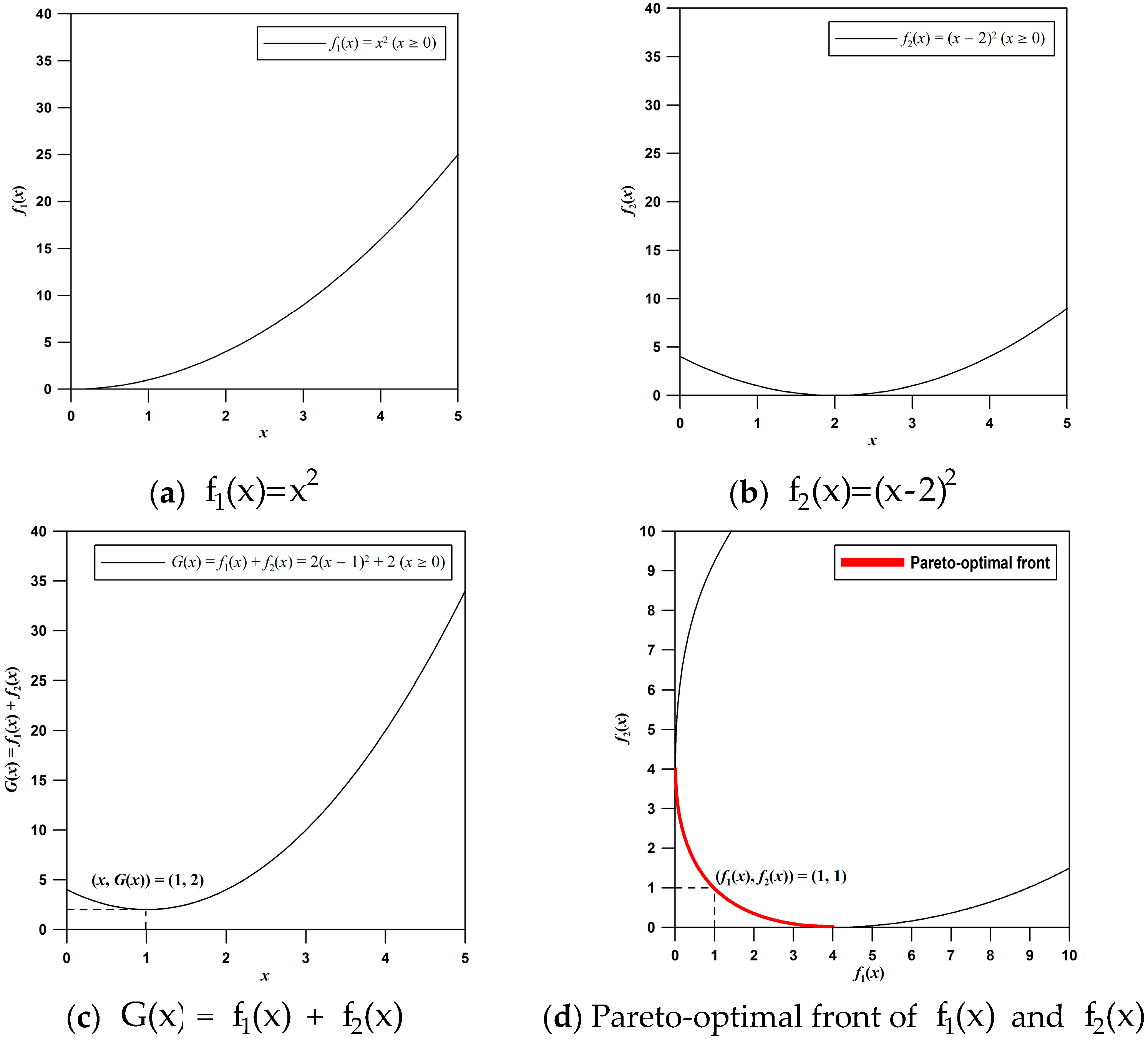
Energies 10 00966 g001
Figure 2. Comparison of global- and multi-objective optimization for a two-objective minimization problem. The global optimum obtained from global-objective optimization is ( x , G ( x ) ) = (1, 2), which is neither the optimum for f 1 ( x ) nor the optimum for f 2 ( x ) . The global optimum is the closest Pareto-optimal solution from the origin under the given weights in objective space. Here, the origin is the ideal but infeasible solution.
Energies 10 00966 g002
Figure 3. Flow chart to design the ES-SAGD process using hybrid NSGA-II algorithm combined with proxy models. The quadratic response surface models are developed from reservoir simulation results of training scenarios of ES-SAGD and then used to evaluate the quality of each ES-SAGD scenario regarding bitumen recovery, cumulative steam–oil ratio, and cumulative solvent–steam ratio. NSGA-II generationally evolves the ES-SAGD scenarios using non-dominated sorting and crowding-distance sorting until the stopping criteria are satisfied.
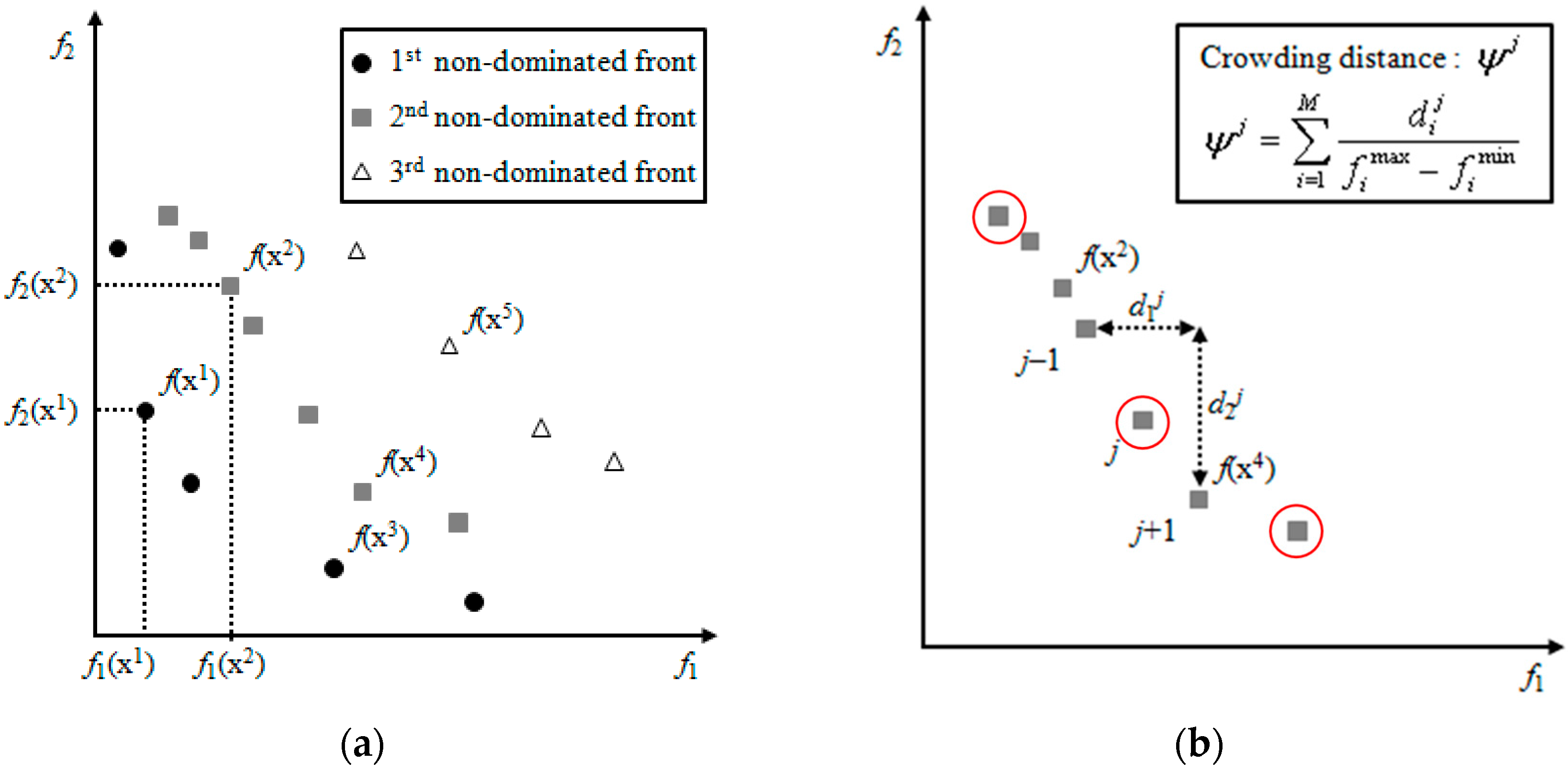
Energies 10 00966 g003
Figure 4. Ranking evaluation using NSGA-II for a bi-objective minimization problem: (a) non-dominated sorting; and (b) crowding-distance sorting.
Energies 10 00966 g004
Figure 5. Configuration of a reservoir model inspired by the McMurray formation in Athabasca oil sands, Canada.
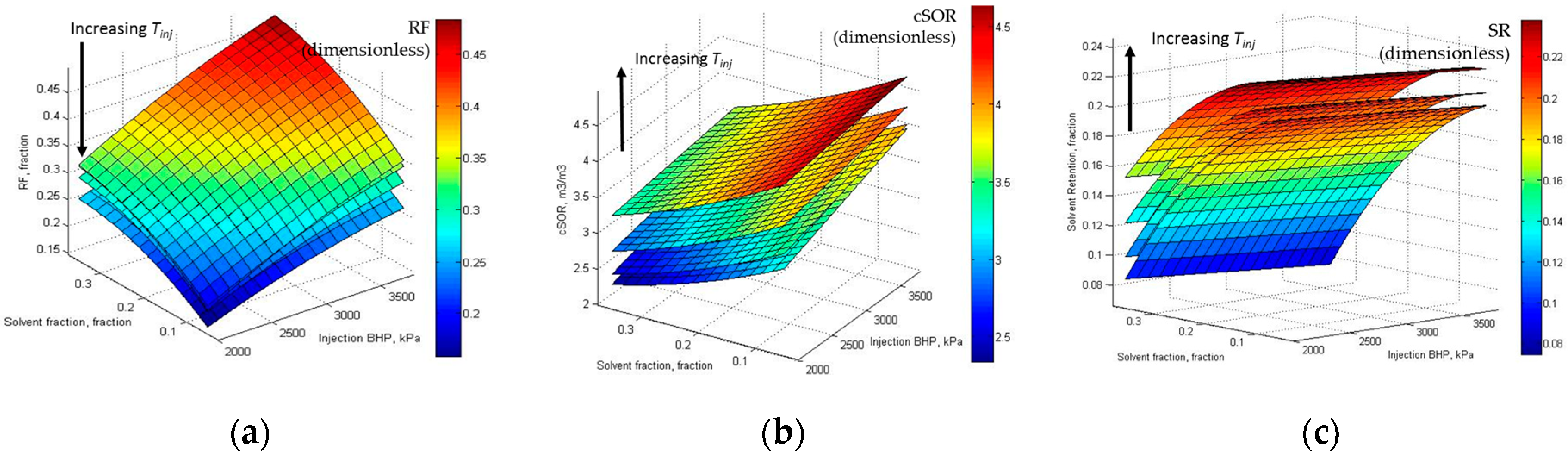
Energies 10 00966 g005
Figure 6. Response surfaces for the three objectives corresponding to four values of pure-steam injection period Tinj (6, 12, 18, and 24 months): (a) recovery factor (RF); (b) cumulative steam–oil ratio (cSOR); and (c) solvent retention (SR).
Energies 10 00966 g006
Figure 7. Surface plots of the three response functions, i.e., RF, cSOR, and SR, in three-dimensional objective space, which corresponds to four values of steam (without solvent) injection period (6, 12, 18, and 24 months).
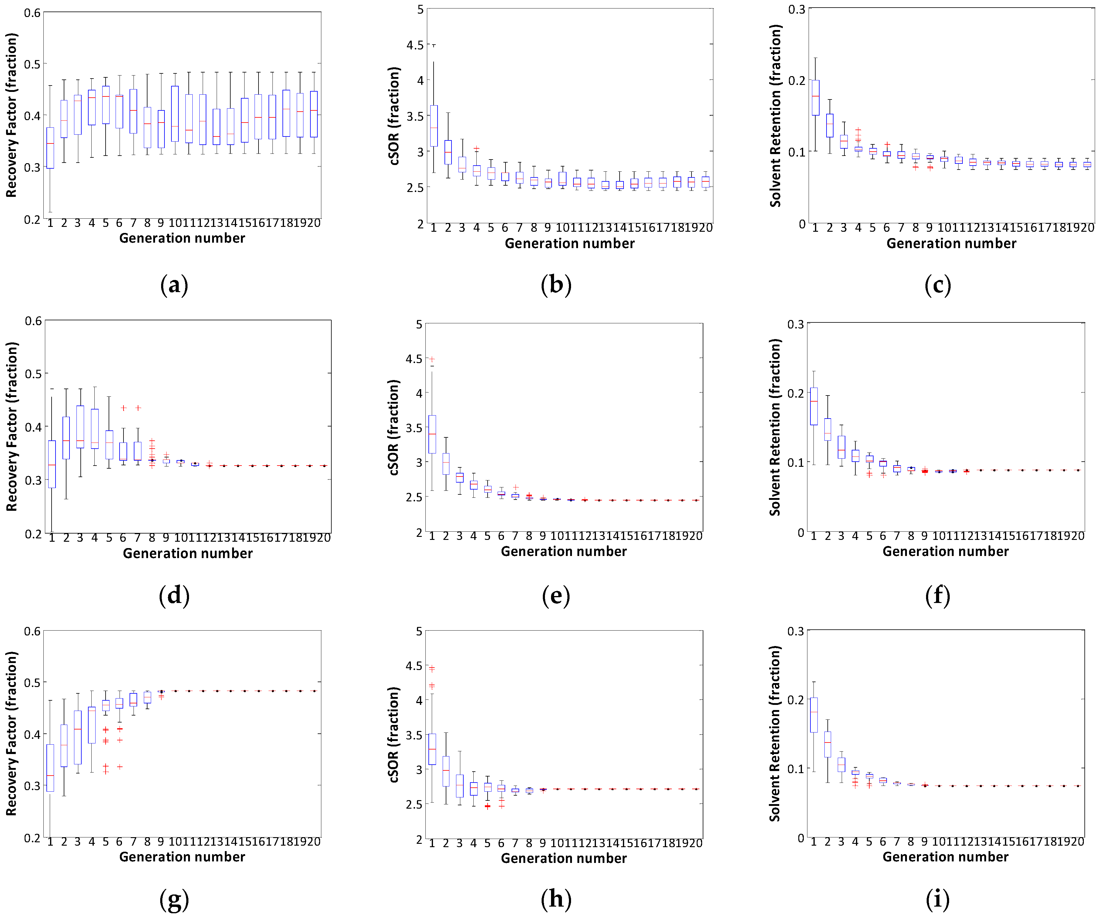
Energies 10 00966 g007
Figure 8. Evolution of performance indicators of the ES-SAGD process obtained by running global- and multi-objective optimization algorithms: (a) Recovery Factor (RF) obtained by invoking NSGA-II; (b) Cumulative Steam–Oil Ratio (cSOR) by invoking NSGA-II; (c) Solvent Retention (SR) by invoking NSGA-II; (d) RF obtained by invoking GA with Equation (12); (e) cSOR obtained by invoking GA with Equation (12); (f) SR obtained by invoking GA with Equation (12); (g) RF obtained by invoking GA with Equation (13); (h) cSOR obtained by invoking GA with Equation (13); and (i) SR obtained by invoking GA with Equation (13).
Energies 10 00966 g008
Figure 9. Projection of decision variables in two-dimensional variable space before and after optimization. The evolved solution set obtained from multi-objective optimization includes the optimum solution obtained from global-objective optimization: (a) Pinj vs. Tinj; (b) Pinj vs. Sfrac; and (c) Tinj vs. Sfrac.
Energies 10 00966 g009
Figure 10. 
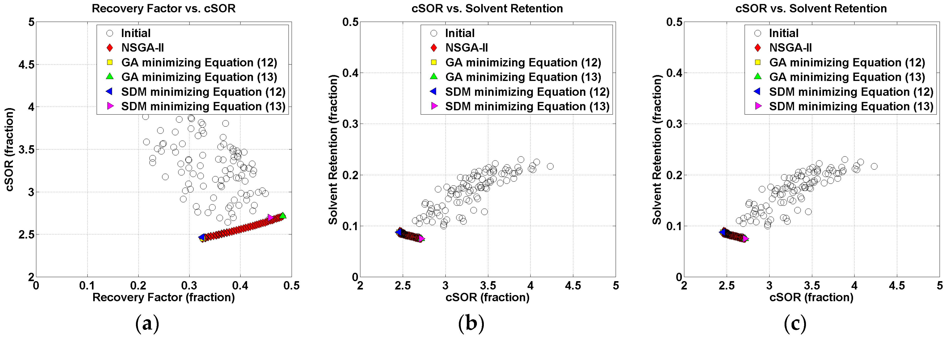
Projection of objective function values in two-dimensional objective space before and after optimization. The evolved solution set obtained from multi-objective optimization includes the optimum solution obtained from global-objective optimization. Positive or negative correlations among the performance indicators of the ES-SAGD process are clearly revealed from the evolved non-dominated solution set: (a) RF vs. cSOR; (b) RF vs. SR; (c) cSOR vs. SR.
Energies 10 00966 g010
Table 1. Reservoir properties used for optimizing the ES-SAGD process.
ParameterUnitsValue
Number of gridblocks (I × J × K)Dimensionless250 × 1 × 100
Size of gridblock (I × J × K)m × m × m1 × 500 × 0.48
PorosityDimensionless0.33
Effective permeabilityDarcy4.2
Initial reservoir temperatureK283.15
Initial bitumen saturationDimensionless0.85
Residual bitumen saturationDimensionless0.1
Specific gravity of bitumen°API8
Molecular weight of bitumenkg/kmole581
Molecular weight of waterkg/kmole18
Thermal conductivity of bitumenW/m/K0.1
Thermal conductivity of rockW/m/K2.85
Thermal conductivity of waterW/m/K0.6
Table 2. Experimental setting of decision variables for proxy modeling and optimization of the ES-SAGD process.
VariableUnitLower LimitUpper LimitStep Size for Proxy ModelingStep Size for Optimization
PinjkPa2000380045050
Tinjmonths62461
Sfracdimensionless0.050.350.0750.01
Table 3. Maximum and minimum values obtained from 100 simulation results used for training proxy models.
Performance IndicatorMinimumMaximum
Recovery factor (RF)0.1580.483
Cumulative steam–oil ratio (cSOR)2.334.64
Solvent retention (SR)0.010.36
Table 4. Regression coefficient vector c and its p-values for each response surface model.
RFcSORSR
ci = 1p-value of cii = 2p-value of cii = 3p-value of ci
ci00.3521.2 × 10−923.2661.7 × 10−920.1782.0 × 10−62
ci10.0641.5 × 10−470.2427.8 × 10−20−0.0062.5 × 10−2
ci2−0.0386.5 × 10−320.4242.1 × 10−370.0233.6 × 10−16
ci30.0609.1 × 10−45−0.4882.1 × 10−40−0.0538.9 × 10−37
ci11−0.0145.6 × 10−60.1121.1 × 10−4−0.0033.7 × 10−1
ci12−0.0026.3 × 10−10.0322.7 × 10−10.0005.5 × 10−1
ci13−0.0088.9 × 10−30.0526.4 × 10−20.0114.4 × 10−1
ci22−0.0114.4 × 10−3−0.0117.6 × 10−10.0050.3 × 10−1
ci23−0.0216.1 × 10−80.2002.6 × 10−80.0093.0 × 10−1
ci33−0.0228.4 × 10−80.0812.3 × 10−2−0.0209.8 × 10−2
Table 5. Coefficients of determination for the three response surface models.
ParameterRFcSORSR
R20.960.930.86
Mean square error3.0 × 10−42.1 × 10−23.0 × 10−3
Table 6. Experimental setting used for multi-objective genetic algorithm.
ParameterValue
Number of generations20
Population size100
Probability of crossover0.9
Probability of mutation0.1
Table 7. Decision variables and performance indicators obtained by running the hybrid multi-objective optimization approach.
Non-Dominated SolutionsRFcSORSRPinjTinjSfrac
Solution 1: with the greatest RF,0.4832.7140.075380060.35
    the greatest cSOR,
    and the lowest SR
Solution 2: with the lowest RF0.3252.4530.086200060.35
Solution 3: with the lowest cSOR0.3262.4510.088200070.35
Solution 4: with the greatest SR0.3322.4630.090205080.35
Table 8. Correlation coefficients between performance indicators obtained from the initial and final solutions of the hybrid multi-objective optimization approach.
Initial Solution Set Final Solution Set
RFcSORSR RFcSORSR
RF1.000−0.494−0.771RF1.0000.997−0.979
cSOR−0.4941.0000.825cSOR0.9971.000−0.973
SR−0.7710.8251.000SR−0.979−0.9731.000

