Study of a High-Pressure External Gear Pump with a Computational Fluid Dynamic Modeling Approach


1
Department of Industrial Engineering, University of Naples Federico II, Via Claudio, 21-80125 Naples, Italy
2
Casappa S.p.A., Via Balestrieri 1, Lemignano di Collecchio, 43044 Parma, Italy
*
Author to whom correspondence should be addressed.
Energies 2017, 10(8), 1113; https://doi.org/10.3390/en10081113
Submission received: 30 May 2017
/
Revised: 26 July 2017
/
Accepted: 27 July 2017
/
Published: 31 July 2017
(This article belongs to the Special Issue Engineering Fluid Dynamics)
Abstract
:A study on the internal fluid dynamic of a high-pressure external gear pump is described in this paper. The pump has been analyzed with both numerical and experimental techniques. Starting from a geometry of the pump, a three-dimensional computational fluid dynamics (CFD) model has been built up using the commercial code PumpLinx®. All leakages have been taken into account in order to estimate the volumetric efficiency of the pump. Then the pump has been tested on a test bench of Casappa S.p.A. Model results like the volumetric efficiency, absorbed torque, and outlet pressure ripple have been compared with the experimental data. The model has demonstrated the ability to predict with good accuracy the performance of the real pump. The CFD model has been also used to evaluate the effect on the pump performance of clearances in the meshing area. With the validated model the pressure inside the chambers of both driving and driven gears have been studied underlining cavitation in meshing fluid volume of the pump. For this reason, the model has been implemented in order to predict the cavitation phenomena. The analysis has allowed the detection of cavitating areas, especially at high rotation speeds and delivery pressure. Isosurfaces of the fluid volume have been colored as a function of the total gas fraction to underline where the cavitation occurs.
1. Introduction
As is well known, external gear pumps are widely used in the fluid power field. These pumps are used in both mobile and fixed applications such as in agriculture, construction machines and hydraulic presses. These machines have many advantages like their compactness and low cost, combined with relatively high efficiency and remarkable reliability, a wide range of operating conditions and structural simplicity. Usually, these pumps are designed to work over a wide range of speeds and high delivery pressures as positive displacement units in hydraulic systems.
The working principle of external gear pumps is very simple. The pump consists of two gears. One is connected to the shaft and is called driving gear; the other one is free and is called the driven gear. These gears are meshed with each other. Chambers are created by coupling the gears with sliding bushing blocks, one for each gear. Two plates connect the gears with the pump housing where, usually, ports are located.
Even if the geometry of these pumps is relatively simple, they are object of many studies addressing the improvement of their performance. This research is mainly focused on the study of all the causes of losses inside the components, through internal fluid-dynamics investigations. Several numerical models are available in literature. These studies (analytical, experimental and modeling) are focused on the prediction of the performance of this pump typology.
Thiagarajan et al. [1] demonstrated improvements of the lubrication ability of external gear machines by designing a micro-surface linear wedge added to the lateral surfaces of the gear teeth. The author showed the reduction of torque loss by adopting a computational fluid dynamics (CFD) numerical approach. The results were confirmed by experimentation.
Vacca et al. [2] studied the operation of spur external gear units with a numerical approach. Then, Pellegri et al. [3] applied the new numerical approach described in [2] with a CFD model, whereby CFD solved the film flow and the lumped parameter model evaluated the overall operation of an external gear pump.
Borghi et al. [4,5], predicted the volumetric efficiency of gear pumps using a mathematical model. The model has been validated with experimental data. Mancò at al. [6] have studied an external gear pump using a lumped parameter approach. Also for this research, model results have been compared with experimental data validating the model.
The improvement of the pump performance can be achieved only by correctly designing the internal fluid dynamic of both lateral plates. These grooves designed in the plates can have several functions such as reducing the noise inside the pump, however grooves connecting volumes at different pressures, can significantly affect the volumetric efficiency of gear pumps if not well designed [5]. The effects of grooves inside plates have also been widely studied by Koc at al. [7]. Borghi at al. [8] also did an interesting analysis on the transient pressure in the meshing volume of external gear pumps.
Many literature studies propose examining gear pumps using 2D modeling approaches with deforming mesh and volume remeshing. However, for the study of pumps like external gear ones, even if the 2D modeling approaches give interesting results, they cannot predict the internal flow behavior like 3D models [9,10]. This depends on the fact that during the operation of an external gear pump, the flow is really complex because of the rotation speeds (typically in the range 500–3000 rpm) and high pressure.
These conditions can cause turbulent flows and sometimes phenomena like cavitation. Yoon at al. [10] did an interesting study on external gear pumps using a three-dimensional approach (with an immersed solid method). The model included the decompression slots that cannot be simulated with a 2D approximation. The model has been used to make interesting considerations on the internal pressure peak, local cavitation, and delivery pressure ripple [11]. They have verified the influence of the gear tip and lateral clearances on the pump performance. Those gaps become crucial in the study of these pumps that, as said, work at a very low speed (500 rpm). Castilla et al. [12], have also built up a complete 3D model of an external gear pump developed with an OPENFOAM Toolbox. No simulation models have been found for the study of cavitation.
In this paper, the authors have studied principally the flow behavior in the chambers and in the meshing zone. The implementation in the numerical model of all the groove and leakages is important to achieve the best accuracy in the prediction of working conditions. The present study is focused on the analysis of the internal fluid-dynamic of an external gear pump using a tridimensional numerical approach. As said, in the literature there are few studies done with three-dimensional simulation tools, and as far as we know, no study has been carried out to fully describe an external gear pump under all operating conditions, even cavitation. The purpose of this research is finding an extremely efficient and fast computational methodology able to predict the overall performance of the components and to allow, by means of monitoring certain points, detecting parameters otherwise difficult to experimentally measure. In addition, this analysis describes a methodology that could be widely used to predict when cavitation occurs inside an external gear pump. This point is of extreme interest for engineers involved in the pump design and optimization phases.
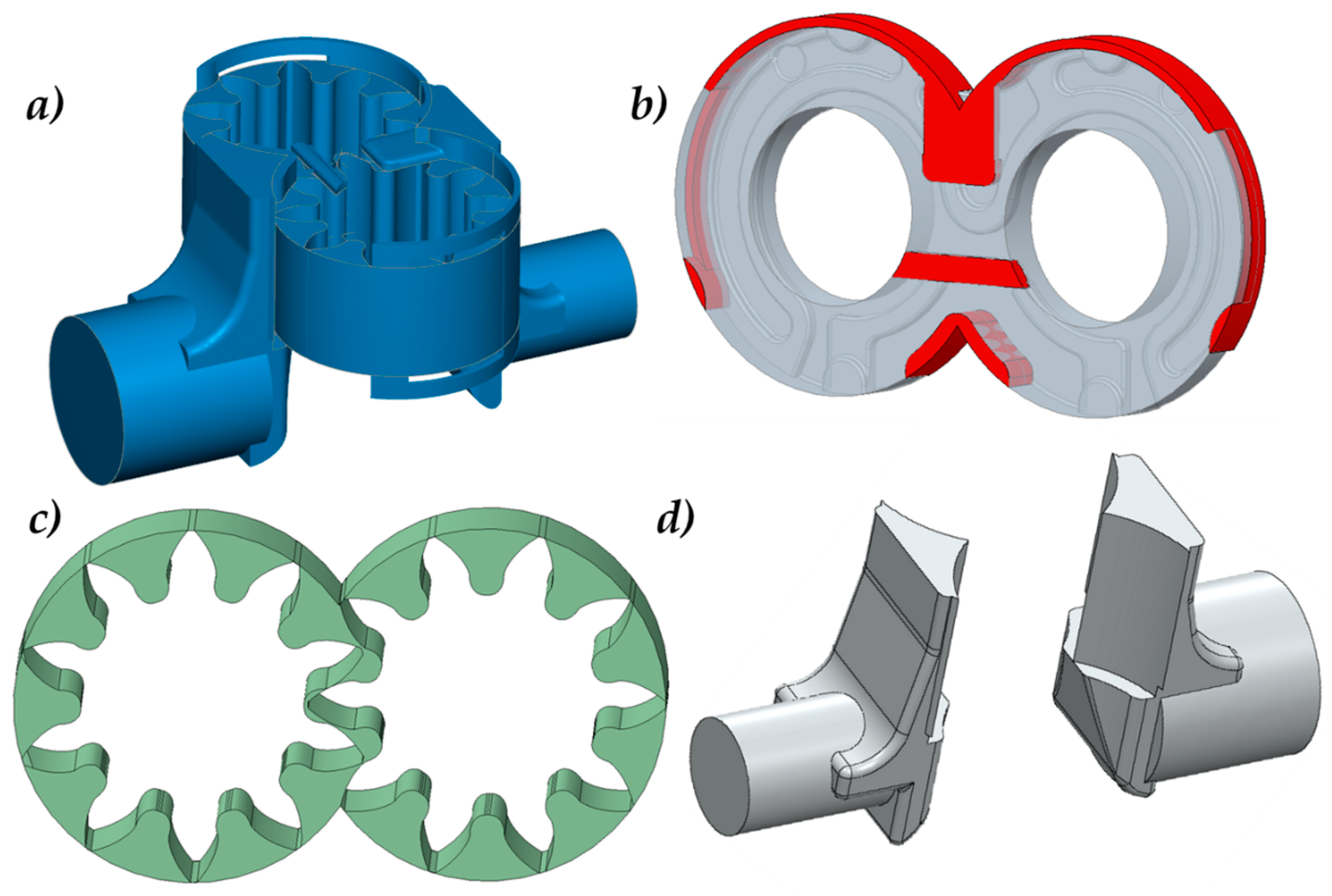
The pump under investigation is the Casappa KP30 (Casappa S.p.A., Parma, Italy), shown in Figure 1a. The pump geometry is shown in the exploded vision in Figure 1b. The pump main features are listed in Table 1. An accurate CFD model has been built up using the commercial code PumpLinx® (Simerics Inc., Bellevue, WA, USA). The entire model of the pump has been created and then validated with experimental data collected by the pump manufacturer.
Flow-rate comparisons have been done at three different delivery pressures and oil temperatures while varying the pump speeds. The model demonstrates an accuracy below 2% for all the analyzed working conditions. The validation of the model has been also done on the pressure ripples. Monitoring points have been located in one chamber of each gear. The post-processing of the pressure inside the chambers underlined the areas under low pressure, especially at high pump speeds.
An analysis on the total volume gas fraction has been performed in order to verify if in the chambers of both gears the pressure goes below the saturation value causing cavitation. For this reason, the model has been implemented with an accurate submodel for the prediction of cavitating conditions.
Particular attention has been paid to the connection plates interposed between the ports and gears. In Figure 2, the geometry of one of them is shown. As said, in the grooves drawn inside plates, during the gear rotation, the pressure reduction can cause cavitation. For this reason, the design phase of plates is important and a CFD modeling approach can help optimize those geometries achieving the best solution. The groove created at the delivery side (underlined with the green rectangle in Figure 2, allows the trapping of the fluid in the high-pressure volume, reducing, as a consequence, the pressure spike in the meshing area. On the other hand, the groove instead allows the filling of the chambers from the suction port. In this way, the pressure drop is reduced, limiting the occurrence of cavitation. Those grooves have also the function to reduce the noisiness of the pump during the operation.
The design of grooves is important because they also cause a loss of flow-rate and, as a consequence, of the pump efficiency. Other grooves have been designed on the plates. These volumes are called high velocity grooves (underlined with the ellipse in blue in Figure 2) and connect a defined number of chambers with the high pressure side. This solution affects the forces acting on the gears. In Figure 2 there is also a rectangular vacancy (underlined with the ellipse in black) that allows the connection to the section port of the pump. This fluid volume will be shown better in Figure 3b. In the second section of the paper, the numerical model of the pump is described.
2. Numerical Model Description
In this section, a numerical model of the studied external gear pump is described. The model has been built up using the commercial code PumpLinx®. Starting from the real CAD geometry of the pump already shown in Figure 1, the fluid volume has been extracted and then meshed. The extracted fluid volume of the entire pump is presented in Figure 3.
The fluid volume has been meshed using a body-fitted binary tree approach. The grid generated with a body-fitted binary tree approach is accurate and efficient because the parent-child tree architecture allows for an expandable data structure with reduced memory storage.
In this architecture of the grid, the binary refinement is optimal for transitioning between different length scales and resolutions within the model. The majority of cells are cubes, which is the optimum cell type in terms of orthogonally, aspect ratio, and skewness, thereby reducing the influence of numerical errors and improving the speed and accuracy. The grid can also tolerate inaccurate CAD surfaces with small gaps and overlaps. Therefore, a body-fitted binary tree approach has demonstrate to be the best methodology to mesh the complex geometry of the pump under analysis. Thanks to the approach adopted, it is possible to create a grid able to take into account the complexity of the geometry, especially in the boundary layer. In fact, also on the surfaces the grid density has been increased without excessively increasing the total cell count. This has been realized using cubic cells, which, as said, are the optimum cell type in terms of orthogonally and improve speed and accuracy. For this reason, in the regions of high curvature and small details the mesh been subdivided and cut to conform it to the surface. From the volume in Figure 3 the mesh has been generated and is shown in Figure 4.
A maximum cell size has been chosen for the grid. This parameter defines the maximum cell size in all the fluid volume. In the same way, a minimum cell size has been fixed to limit the minimum dimensions of all cells. Fixing this parameter means that no cell side can be smaller than the minimum cell size. Another important parameter must to be set, which defines the size of cells on surfaces.
Different techniques are available for the treatment of a moving mesh. For positive displacement pumps, it is necessary to use a moving/sliding methodology whereby the stationary and moving volumes are meshed separately. The code, therefore, allows for the simultaneous treatment of moving (gear chambers) and stationary (like suction and delivery ports and grooves in the plate geometry) fluid volumes. Each volume has been connected to the others via an implicit interface called mismatched grid interface (MGI). Each MGI, due to deformations and motion, is updated at each time-step.
2.1. Study of the Gap between Teeth
Before describing the model results obtained it is important to proceed with an analysis on the sizing of the gaps between teeth. This study becomes crucial to correctly predict the performance of an external gear pump. Therefore, in the following a preliminary study done choosing the clearances between teeth of gears is presented.
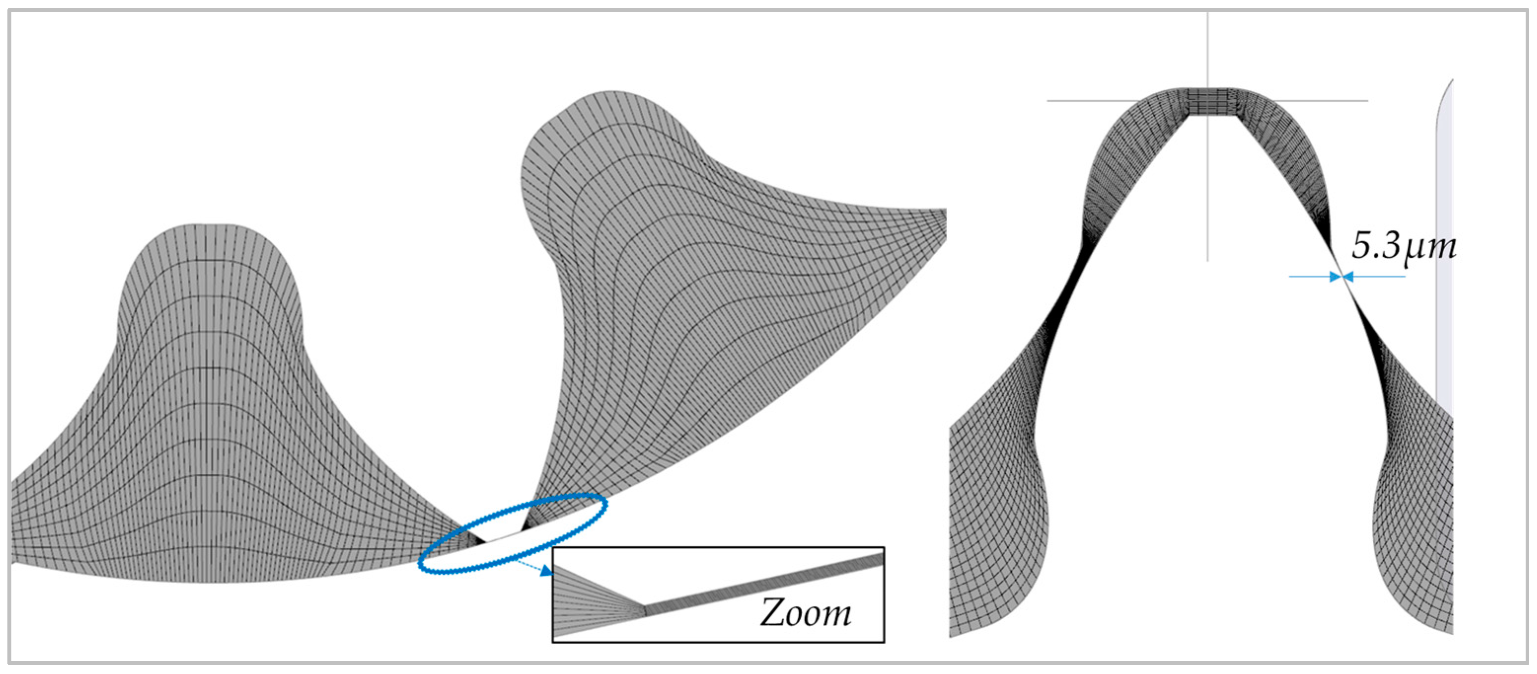
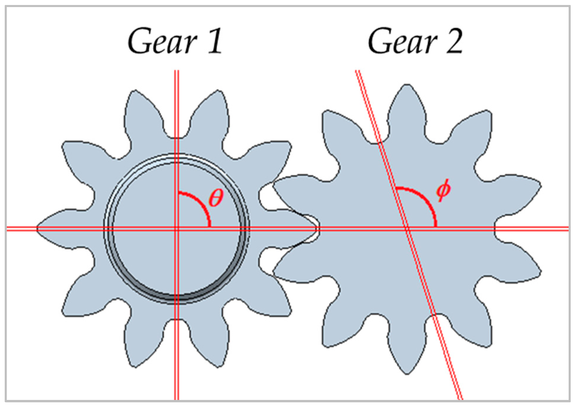
As shown in Figure 5, the minimum gap between teeth is 5.3 μm. This gap value has been defined after a analyzing the pump geometry and the angles θ and φ in Figure 6). The angle θ defines the “driving gear” (Gear 1 in Figure 6) position while the angle φ is referred to the “driven gear” (Gear 2 in Figure 6). The angle φ is defined as function of the angle θ and the number of teeth z of each gears. This angle ideally is calculated as follows:
Looking at Figure 6, in this configuration gears are perfectly meshing but not in contact. However this meshing is not real, because, as well know, there is no gap between gears in a real working pump. Therefore, in order to correctly reproduce real working conditions, where contact occurs, Equation (1) must be implemented including the shift angle φ. Equation (1) becomes:
2.2. Mesh Sensitivity Analysis
A mesh sensitivity analysis has been done on the model by changing the size of the grid. This analysis should be always done in a CFD study to define the best grid for each application and to correctly predict the real working conditions of the pump. Therefore, in this section a mesh sensitivity showing the effects on the model results of variation for example of the clearances between teeth and sliding bushing blocks is presented.
Fluid volumes have been slit in six parts: inlet port, outlet port, outlet high speed grooves, inlet low noise grooves, outlet low noise grooves e rotor. Each volume has been connected to others, as said, via the “MGI” interface (see Figure 4b). Table 2 clarifies the importance of the mesh sensitivity analysis in a CFD study.
A first step has been done analyzing the influence of the grid on the boundary layers. Two different meshes have been created by changing the grid parameters in the boundary layers. These models are called “Mesh 1” and “Mesh 2” where the second one has a finer grid size.
In Table 2, the percentages of error between the suction and delivery flow evaluated by the model are reported. The simulations in Table 2 have been run at 1500 rpm and for two delivery pressures: 50 and 200 bar. As shown in the Table 2, the ΔQ% of both models “Mesh 1” and “Mesh 2”, as expected, increases with the delivery pressure.
As shown in the table, improving the quality of the mesh in the boundary layers, the ΔQ% between suction and delivery ports becomes closer to each other. In fact, the reductions from simulations “1” and “2”, for both pressure levels, are significant.
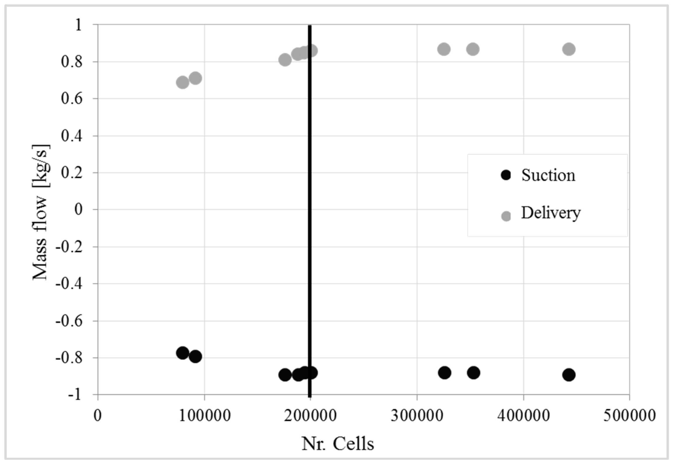
After the analysis on the boundary layers, the mesh has been studied improving the quality. Nine models have been created increasing the number of cells. In Figure 8, a comparison of the suction and delivery mass flows is shown. Looking at the graph, it is clear that only with a grid above 200,000 cells does the solution become stable. Each point in Figure 8 corresponds to a model built up with a different grid size.
Simulations have been run, as already said, has been run on an Intel® Xeon® X5472 CPU @ 3.00 GHz (two processors) with 24 GB RAM. As we know, upon increasing the number of cells the simulation time increases as well. From the analyzed case, the time goes from half an hour for the first point in Figure 8 to 10 h of the last model of almost 500,000 cells. Therefore, in order to achieve the best compromise between accuracy and computational time, the final model consisted of 200,000 cells which is the point underlined in Figure 8.
2.3. Model Setup
The standard 𝑘-𝜀 turbulence model has been adopted because for this specific problem it has proven to be accurate. The 𝑘-𝜀 model is a robust method demonstrated to provide good engineering results. As well known, in the literature there are other resolution methods more accurate than the 𝑘-𝜀 model and RNG 𝑘-model (RNG, LES, or DES, etc.). However since the losses due to the viscous stresses are negligible compared to pressure forces the 𝑘-𝜀 model can be chosen because it is numerically robust, computationally efficient and it provides good accuracy. In fact, in this application, where the computational time is close to 10 hours per revolution, the adoption of a higher order turbulence model would have increased the computational time with no relevant improvement of the results. The authors of this paper have already used this strategy for many other similar analyses confirming the accuracy of the solutions obtained [13,14,15,16,17,18,19,20,21].
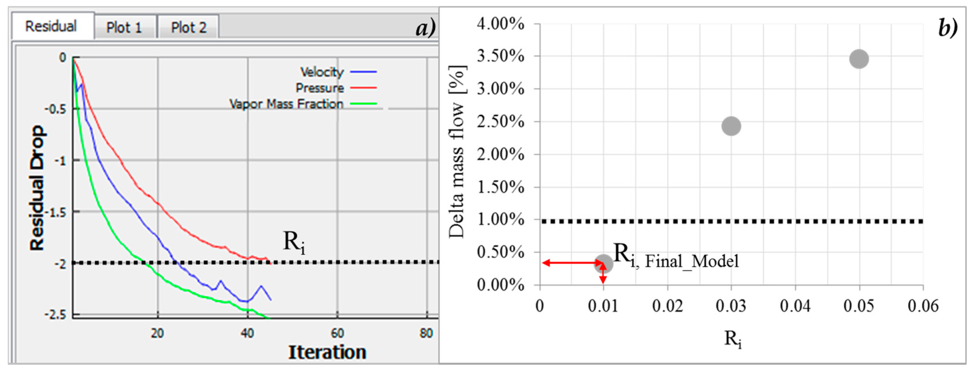
An analysis on the convergence criteria have been done to achieve the best accuracy results. “Ri” is the residual drop referred to the “i-th volume”. It is defined as the difference between the obtained results, for the selected volume, during two subsequent iterations. The correct solution convergence is realized when all the residuals go below the defined Ri.
For all the simulations, the convergence criteria for the pressure, velocity and the vapor mass fraction is 0.01 as shown in Figure 9a. Figure 9a, in fact, presents the trend of the residual drop for each variable in a single time-step. As shown, residuals go below 0.01 (settled Ri.).
These values have been demonstrated to be suitable for this application. However, a study on the convergence criteria has been also performed varying the Ri. As example, in Figure 9b the Ri is shown as function of the delta mass fraction (%) between the pump inlet and outlet mass flows. As shown, the Ri has been varied from 0.01 to 0.05 with steps of 0.02.
The maximum error on the delta mass fraction between the pump inlet and outlet mass flows has been fixed at 1%. It has been demonstrated that the best solution can been achieved with a Ri of 0.01 (Figure 9b). Other analyses have been run reducing the Ri for the to lower value without improving the delta mass flow percentage.
Before running simulations, it is important to underline that in this study the model has been built up including an accurate submodel able to predict cavitation. In the following subsection the study of cavitation inside an external gear pump has been done. In fact, one of the targets of this research was to detect cavitation, in order to predict the worst working conditions for the pump.
Since one of the aims of the research is the investigation on the ability of the pump to avoid cavitation, the model has been equipped with a robust submodel, available in the code, able to predict with high accuracy cavitating conditions. The chosen cavitation module accounts for all three important real liquid properties: cavitation, aeration, and liquid compressibility. This model builds on the work of Singhal et al. [22]. A module is used to predict the aeration and cavitation in a liquid system, therefore allowing for the calculation of cavitation effects, when the pressure in a specified zone of the fluid domain falls below the saturation pressure and vapor bubbles form and then collapse as the pressure rises again [22]. Many physical models for the formation and transport of vapor bubbles in liquids are available in literature, but only few computational codes offer robust cavitation models. This is due to the difficulty on handling gas/liquid mixtures with very different densities. Even small pressure variations may cause numerical instability if they are not optimally treated [22].The original cavitation model proposed by Singhal et al. describes the vapor distribution using the following formulation [13,14,15,16,22]:
where Df is the diffusivity of the vapor mass fraction and σf is the turbulent Schmidt number. In the present study, these two numbers are set equal to the mixture viscosity and unity, respectively. The vapor generation term, Re, and the condensation rate, Rc, are modeled as [13,21]:
in which the model constants are Ce = 0.02 and Cc = 0.01.
The model by Singhal et al. has been extended to include non-condensable gases, finite rate and equilibrium dissolved gas. The fluid model, in addiction, accounts for liquid compressibility. This is critical to accurately model pressure wave propagation in liquids. The liquid compressibility is found to be very important for a high-pressure system and the systems in which water hammer effects are relevant.
3. Model Validation
The pump has been tested on a dedicated test bench at Casappa S.p.A. The test bench is shown in Figure 10. Simulations have been run under the same conditions tested in the lab with pump speeds of 1000, 1500 and 2500 rpm, oil temperatures of 50 and 80 °C and delivery pressures of 50, 150 and 250 bar.
The test bench layout is shown in Figure 10b. There are two strain gauge sensors P1 and P2 (both from WIKA®, Lawrenceville, GA, USA, scale: 0–40 bar and 0.25% FS accuracy) and P2 at the delivery side (by WIKA®, with a scale of 0–400 bar and an accuracy of 0.25% FS). The pressure sensor P4 is piezoelectric (made by KISTLER®, Winterthur, Switzerland, scale: 0–1000 bar, 140 kHz natural frequency, 0.8% FS accuracy) while the traducer P5 is piezoresistive (ENTRAN®, Strainsense Ltd, Milton Keynes, UK, scale: 0–350 bar, 450 kHz natural frequency, compensated temperature, 0.5% FSO accuracy).
The flow-rate mater Q1 is a VSE® VS1 (VSE.flow, Neuenrade, Germany), scale 0.05–80 l/min, 0.3% measured value accuracy. There is an HEIDENHAIN®, ERN120 θ encoder (HEIDENHAIN, Traunreut, Germany), 3600 r/min, a limit velocity 4000 r/min and a period accuracy of 1/20.
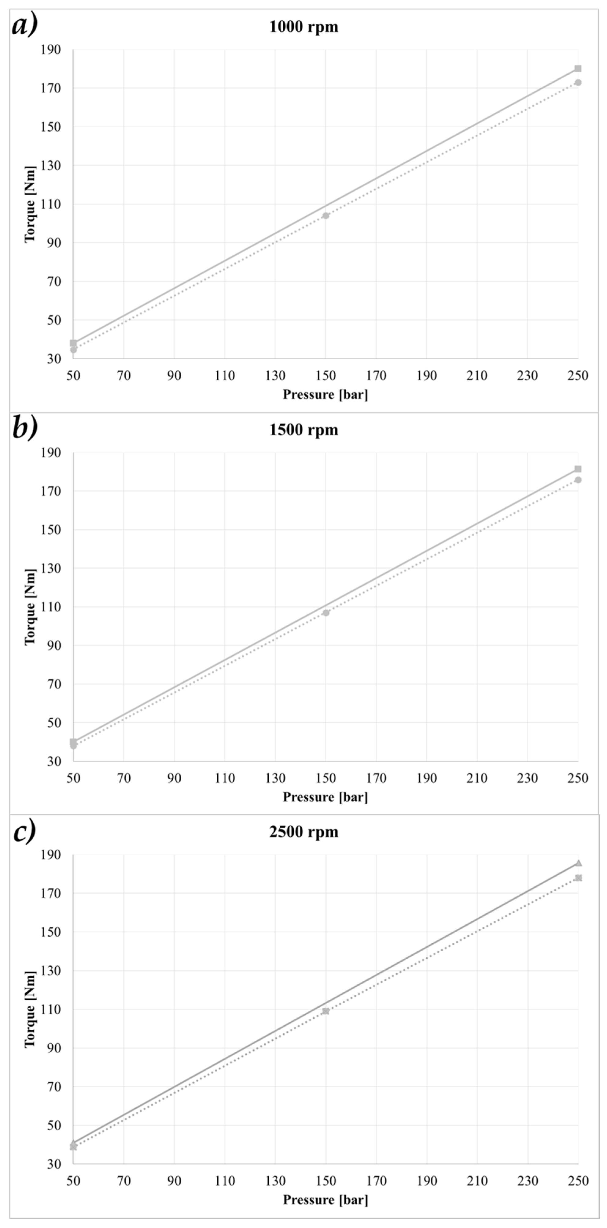
In Figure 11a–c, a first comparison between model and experimental data is shown for three different pump speeds: 1000, 1500 and 2500 rpm. In the graph, the continuous line are the experimental data while the dashed ones are the simulation results.
Simulations and test, as said, have been done for three delivery pressure conditions: 50, 150 and 250 bar. The comparisons have been done on the torque requested on the driving gear (gear 1 in Figure 6).
By analyzing Figure 11, it is possible to appreciate that the model results are really close to the experimental data. However, there is a gap between model and experimental data that depends also on the fact that the model does not consider torque due to mechanical friction.
The experimental data in thick lines represents the absorbed torque by the pump measured by a torque meter. This means that experimental data takes into account, of course, the “hydraulic” component of torque (volumetric efficiency) even of all the friction (mechanical efficiency). This is the reason why the simulation results are lower than the experimental data. In Figure 12 the delta torque between experimental and model results is presented. This ΔC represent the toque lost due to friction.
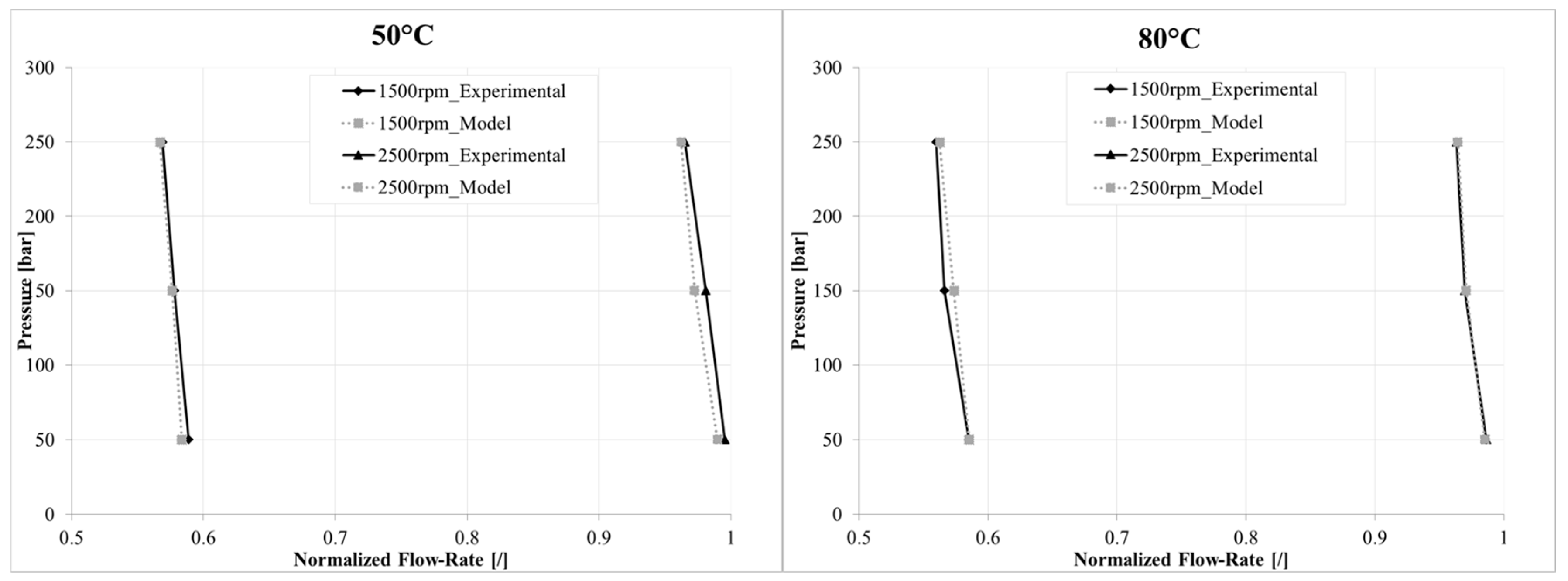
Model validation has been done also comparing at the delivery flow-rate varying the delivery pressure. This comparison is shown in Figure 13 at the oil temperatures of 50 and 80°C and at pump speeds of 1500 and 2500 rpm.
It can be noticed that delivery flow rate decreases by increasing the delivery pressure for both the model and experimental data; the error percentage between model and experimental data is always below 2%.
4. Model Results
The validated model has been analyzed in order to study the pump in depth. A three-dimensional CFD modeling approach, as said, has many advantages. In fact, considering the real geometry of the pump, it is useful to visualize parameters that are impossible or onerous to obtain experimentally such as the velocity magnitude of the fluid in leachates.
Figure 14 shows a first result of the numerical model with the velocity magnitude countering through the leakages between gears and the static body. The area under investigation in the pictures is shown in Figure 14c. In fact, figures refer to the leakages between the first pressurized chamber and the last chamber at low pressure.
Figure 14a,b, in particular, show the results in the gaps by increasing the pressure from 50 to 250 bar for oil temperatures of 50 and 80 °C, respectively, at the same pump speed. The velocity magnitude scale in all figures is always in the 0–13 m/s range.
In Figure 14a, by comparing graphs at the same oil temperature it is possible to distinguish the flow velocity magnitude profile through gaps. In fact, as consequence of the higher pressure drops between the two following chambers (from 50 to 250 bar), the flow velocity through the gap between the tooth and the pump housing increases and, as shown in pictures in Figure 13, flow becomes a jet.
Looking for example at Figure 14a, the flow velocity through the gap with a delta pressure of 50 bar is below 5 m/s. It increases in correspondence of the connection between the gap and the chamber at the lower pressure. This velocity profile is, of course, quite similar with a higher pressure drop, however the values increase. For a Δp of 150 bar the maximum velocity value registered in the analyzed fluid volume is of almost 9 m/s. It becomes 13 m/s for the delta pressure of 250 bar.
It is interesting to underline the effect of the Toil on the flow velocity and as consequence, on the pump volumetric efficiency. For all the analyzed Δp, the velocity at 50 °C is lower than for an oil temperature of 80 °C. This depends by modification of the fluid properties with the temperature.
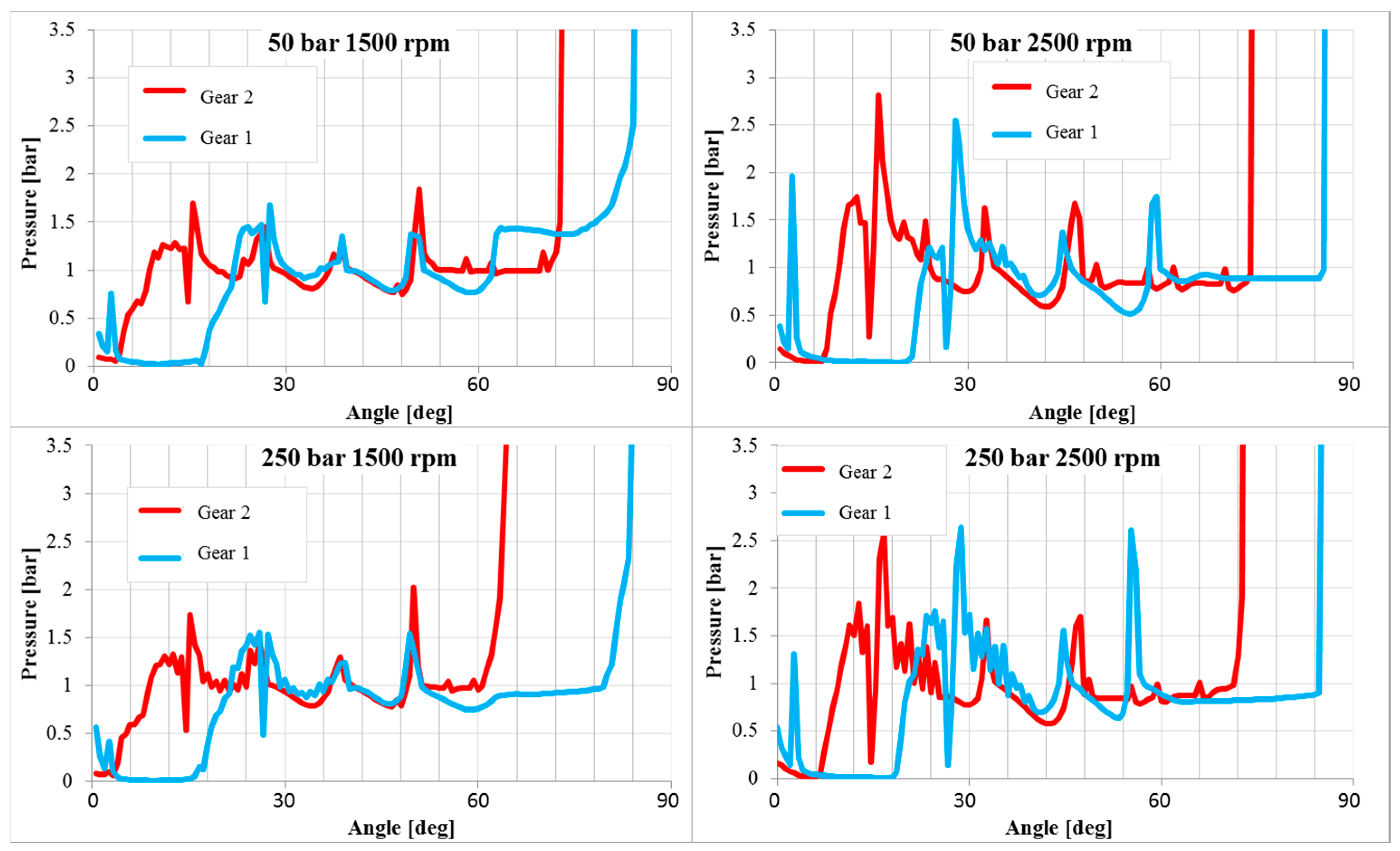
In Figure 15, the pressure evolutions inside the chambers are diagrammed for a shaft revolution at the operating condition listed below:
- Oil temperature of 50 °C
- Pressure drop of 50 and 250 bar
- Pump speed of 1500 and 2500 rpm.
As is well known, it is also possible to obtain experimentally the results in Figure 15, however it is not easy. Therefore, the best solution is to obtain these important data with modeling techniques.
Data shown in graphs of Figure 15 allow evaluating the pressure evolution inside a chamber in rotation for each gear. In particular, the lines in red refer to the chambers of the gear 1, while the blue ones correspond to gear 2.
The graphs can be interpreted as follows. From the suction port the flow fills the generic chamber (obtained by coupling the two gears) and is compressed. Looking at Figure 15, it is clear that each chamber has a pressure evolution during the 360 degrees but the low-pressure zone has a lower angular extension. It is, in fact, more or less 90 degrees and depends by the pump geometry.
As expected, when the chamber is connected to the delivery port, it has an oscillating pressure around the delivery value (in this case 50 and 250 bar). The pressure is smoother around the mean value with a lower pump speed (1500 rpm). At 2500 rpm instead the oscillations around the mean value are high for both delivery pressures. The pressure spikes inside the chambers, at the higher delivery pressure level, are clear for both gears’ fluid volumes. Those investigations, especially the evaluation of the spikes values, are really important for engineers to design or optimize a pump.
The results in Figure 15 are also of extreme interest by visualizing the pressure-axis in the range 0–3.5 bar and reducing the angle-axis to the only the degrees of connection with the pump suction side. In this way, it is possible to appreciate the behavior of the pressure when the chamber is connected to the suction port. These results are shown in Figure 16, providing a preliminary investigation of the cavitation phenomena. Cavitation, however, it analyzed in depth in Section 5.
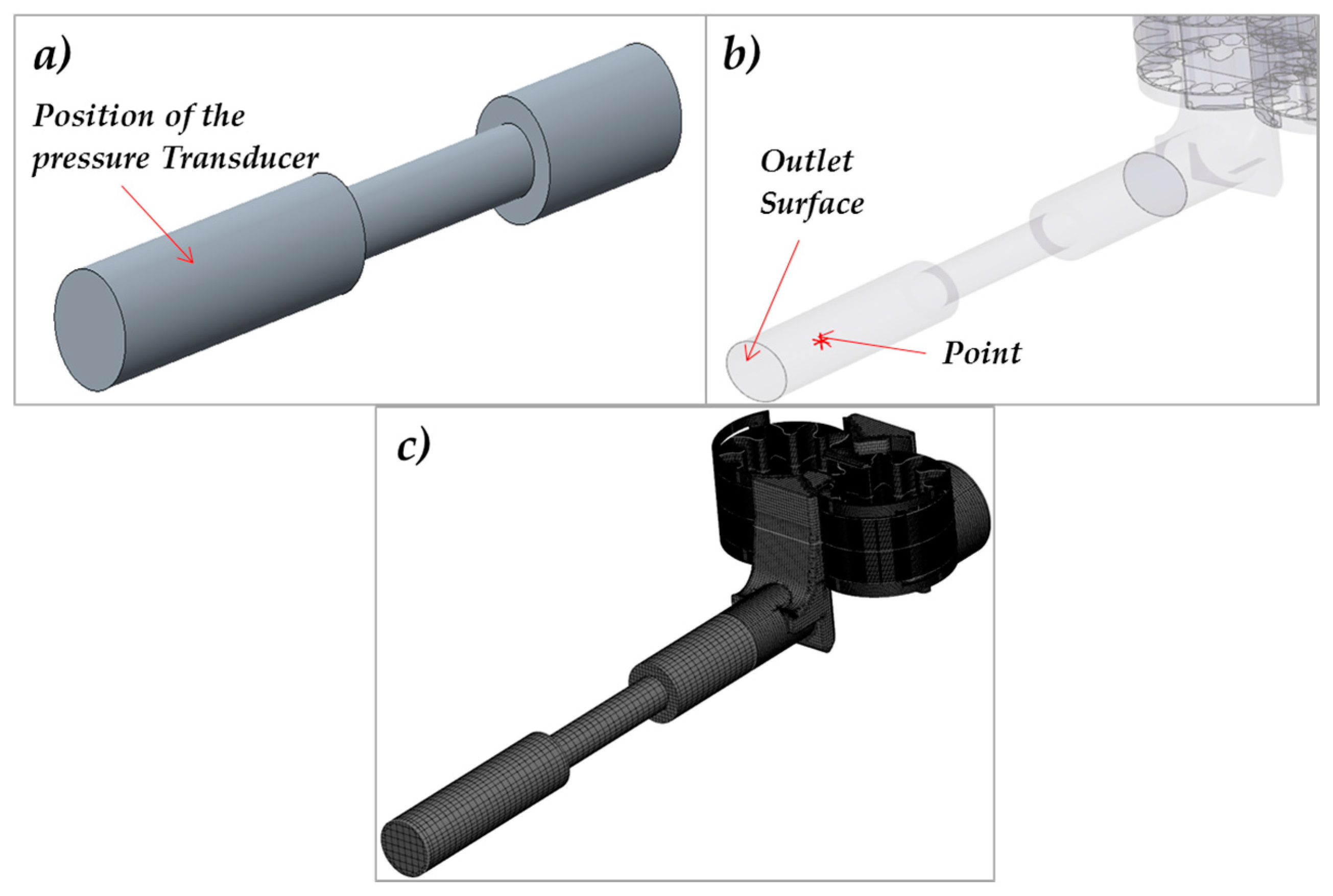
However before studying the cavitation phenomena a study of the pressure ripples at the delivery side of the pump has been performed. For this reason the model has been implemented adding a supplementary volume in accordance with the experimental tests. This duct has the same geometry of the real one, installed on the test bench in order to correctly follow the experimental delivery pressure ripples. The geometry of the duct is shown in Figure 17a while in Figure 17b the final model is presented. In the model a monitoring point located at the same position of the pressure transducer has been added and a section set like the real lamination valve of the test bench has been added too. This section therefore simulates the lamination valve, and for this reason the entire model simulated with high accuracy the pressure waves inside the delivery duct.
During the tests a valve has been located close to the pump delivery in order to amplify the pressure ripples. As consequence, the model has been implemented by adding a calibrated orifice. The additional fluid volume has been inserted to replicate the real experimental setup. In Figure 17, the entire model of the pump is shown, including the fluid volume of the calibrated orifice. Simulations have been run with the model in Figure 17 and the model results have been compared with the experimental data.
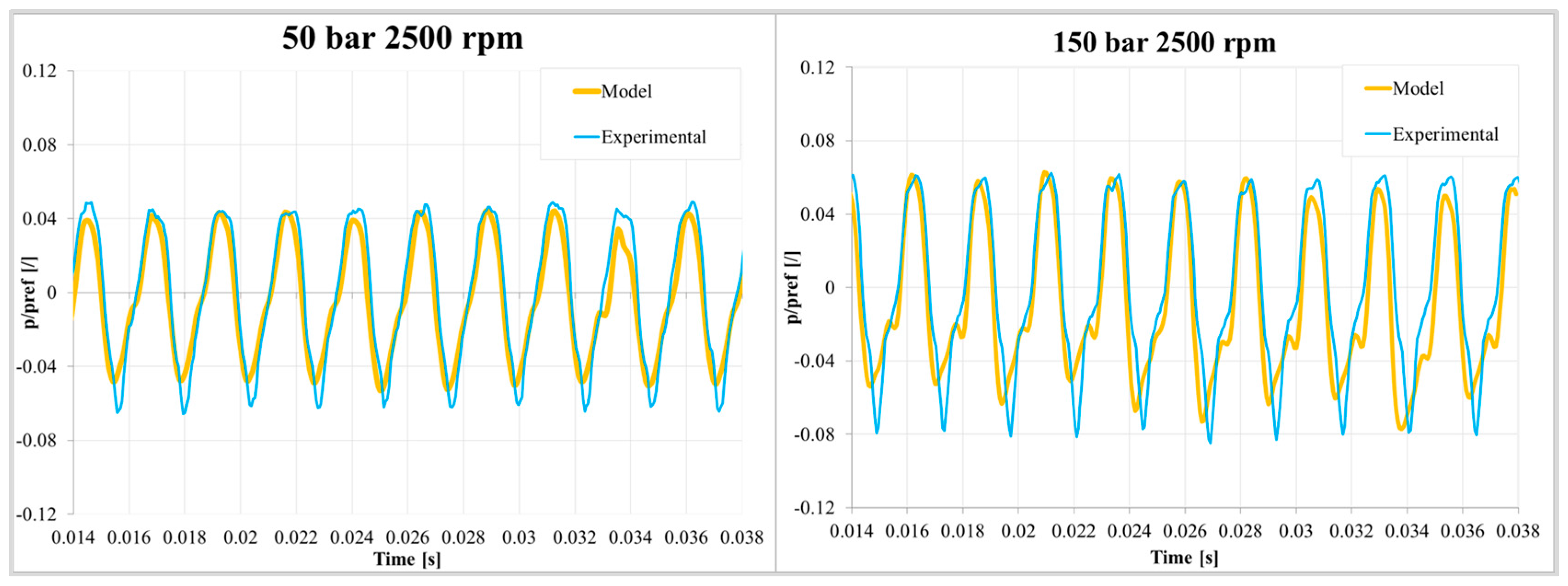
The monitoring point for the simulation has been located in the same position of the pressure transducer installed on the test bench, as shown in Figure 17b; in that point the pressure ripple has been both measured and calculated. Comparisons have been done at two rotational speeds and three pressure levels at 50 °C (see Figure 17). The diagrams in Figure 18 have been normalized to a reference pressure.
As said, the model results in Figure 18 have been obtained changing the delivery pressure at 2500 rpm. Comparison between the model and experimental data shows a good agreement in all the analyzed conditions, confirming the accuracy of the numerical model. The results, in fact, show that the timing and ripples have the same amplitude as the experimental data.
Pressure ripples show that the amplitude of the oscillation increases with the delivery pressure. In the graphs the y-axis has been fixed, therefore, looking at the ripples, it is clear that by increasing the delivery pressure the amplitude increases as well. This happens for both pump speeds.
5. Cavitation
In this section, the model results have been analyzed verifying if cavitation occurs under particular pump-operating conditions. The model, as already said in the corresponding section, includes the capability of prediction of the occurrence of cavitation. Thanks to the three-dimensional visualization of the total gas volume inside the pump, it is possible also to find when the cavitation occurs and where bubbles are located. The study of this phenomenon becomes important for engineers in the pump design and optimization phases.
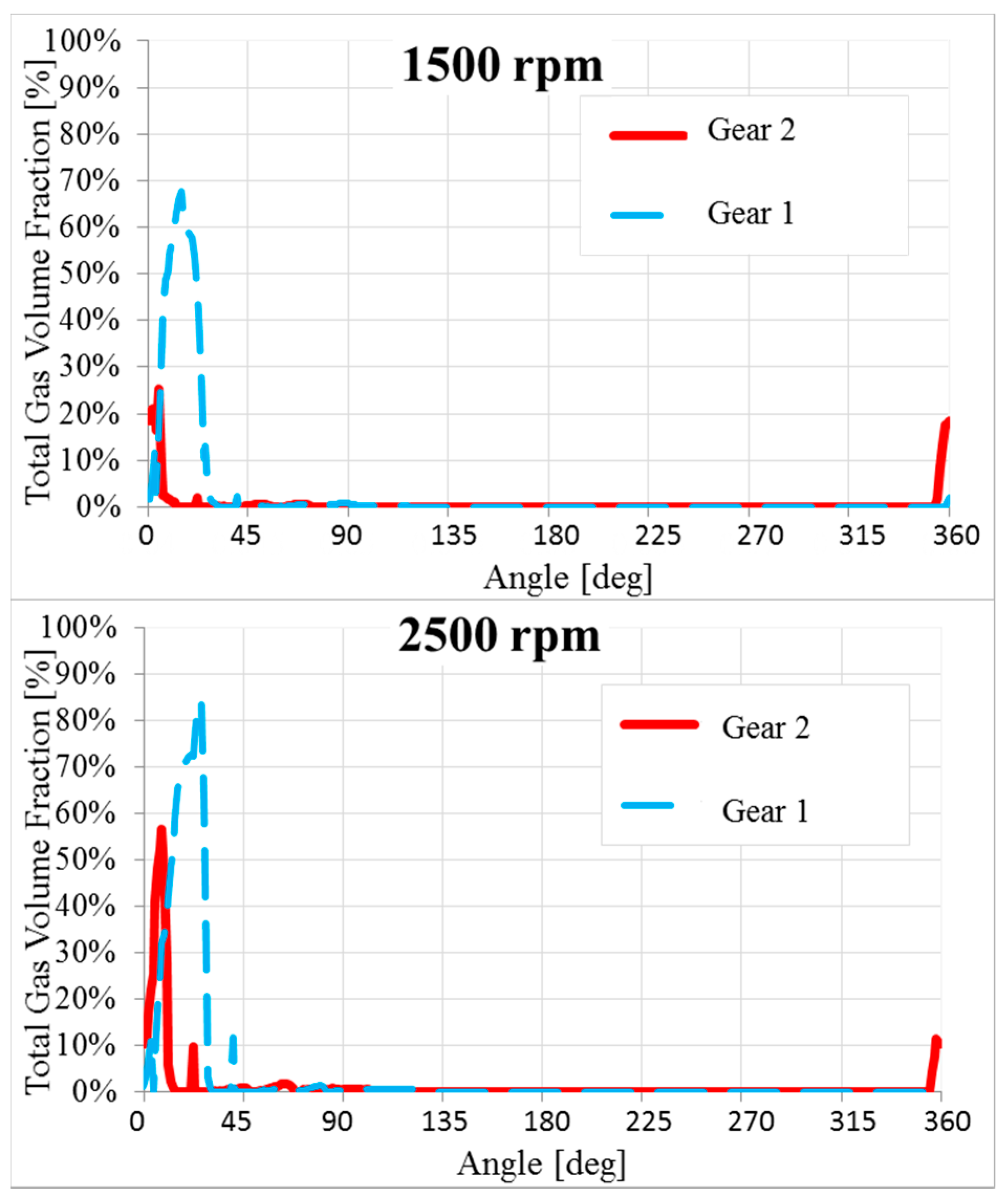
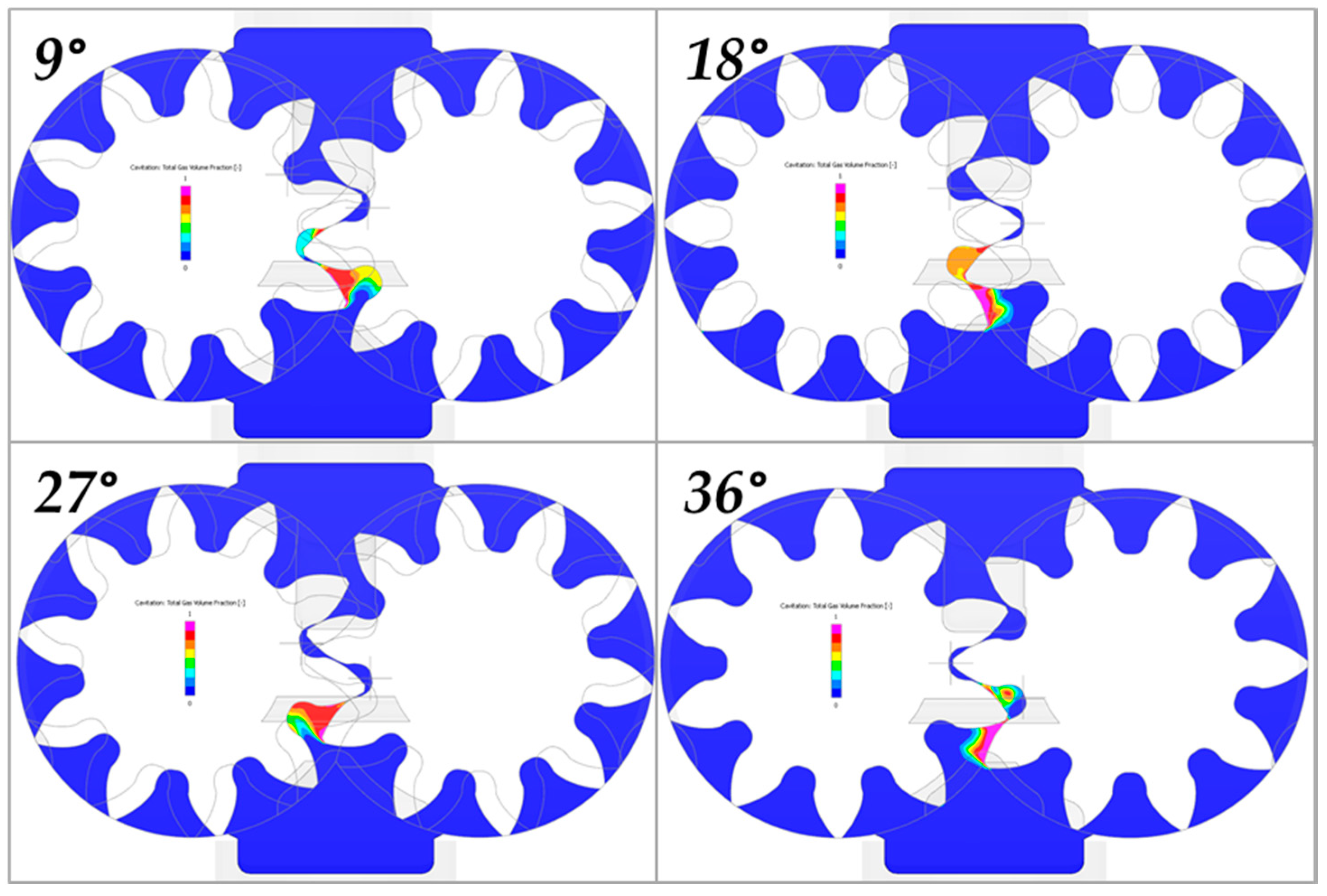
In Figure 19, a front view of the pump is shown. The volume is colored as a function of the total gas fraction that varies in the range 0–1. The gas volume fraction is the volume fraction of the free non-condensable gas (NCG) in a liquid for a selected volume. In Figure 19, there are presented four sections relative to gears rotations of θ = 9°, 18°, 27° and 36°. The simulation has been done under fairly critical conditions for the cavitation: 2500 rpm and 250 bar.
Areas in blue correspond to a concentration of free gas equal to zero while areas colored in magenta are at a percentage of gas of 100%. As shown, the areas in magenta are located in areas where the rotating chamber, from the condition of minimum, starts to increase its volume. Therefore, in correspondence with the meshing area, an intense and sudden cavitation occur. As well known, this phenomenon causes noise and damage to parts and therefore must be avoided. Figure 20 shows two diagrams of the total gas volume fraction inside the chambers of gears. The total gas volume fraction, as said, varies in the range 0–100%.
Signs of cavitation could be appreciable for values higher than 80%. Even if the total gas fraction in the chamber of the driving gear at 2500 rpm has a spike between 0° and 45° this pump demonstrates to not be subject to cavitation, even under critical operating conditions. However, the methodology described in this paper is demonstrated to be suitable because it offers the opportunity to fully study the complex fluid dynamics of external gear pumps. Results showing cavitation are really important for the optimization of a pump. Therefore, a CFD modeling analysis becomes fundamental in the design phase of components to achieve the best performance for all working conditions.
6. Conclusions
A three-dimensional CFD study a high-pressure external gear pump has been descried in this paper. The model has been realized based on a geometry of a pump manufactured by Casappa S.p.A. The model has been built up using a commercial code including accurate tools to predict the flow turbulence and cavitation. Leakages have been taken into account in order to correctly estimate the volumetric efficiency of the pump. The final model has demonstrated to achieve an accuracy close to 1%.
Model results have been compared with experimental data obtained on a dedicated test bench by the pump manufacturer. Thanks to the good agreement of the data the model has been run under some conditions (such as at high pressure value) which are very challenging from a modeling and numerical point of view. Simulations have found that at the higher pressure and speeds the pump has a tendency to cavitate. For this reason, monitoring points have been located inside the chamber volumes of both gears.
The pressure behavior underlined that the pressure, especially inside the driving gear chamber, goes below the oil saturation pressure. This has been confirmed by visualizing the total gas fraction distribution in sequential images in a pump cross-section. This study summarized a methodology able to completely describe the operation of pumps such as external gear pumps. All the working parameters have been analyzed and, where possible, compared with experimental data. Research has confirmed the importance of CFD, which can be a valuable instrument for engineers to study some working anomalies like cavitation.
Acknowledgments
This research is a result of a research collaboration between the Fluid Power Research Group (FPRG) of the Department of Industrial Engineering of the University of Naples “Federico II” and Casappa S.p.A. We appreciate the technical contribution from Federico Monterosso and Micaela Olivetti of OMIQ s.r.l.
Author Contributions
Emma Frosina and Manule Rigosi built up the model. Adolfo Senatore supervised the study. Emma Frosina wrote the paper.
Conflicts of Interest
The authors declare no conflict of interest.
Nomenclature
| ceq,k | Coefficient |
| CFD | Computational fluid dynamic |
| Cc | Cavitation model constant |
| Ce | Cavitation model constant |
| Df | Diffusivity of vapor mass fraction |
| dS | Infinitesimal surface, m2 |
| fv | Vapor mass fraction |
| fg | Non-condensable gas mass fraction |
| Gt | Turbulent generation term |
| MGI | Mismatched grid interface |
| Ndriving | Number of the teeth of the Gear 1 |
| n | Pump velocity rotation, rpm |
| pu,k | k-th inlet pressure, bar |
| pd,k | k-th outlet pressure, bar |
| ps | Oil supply pressure, Pa |
| Qteo | Theoretical flow-rate, l/min |
| Qreal | Real flow-rate, l/min |
| Ri | Residual drop |
| Re | Vapor generation rate |
| Rc | Vapor condensation rate |
| rpm | Pump speed |
| S’ij | Strain tensor |
| Toil | Oil temperature, °C |
| V | Pump displacement, cm3/rev |
| Vi | i-th volume, m3 |
| Greek Letters | |
| β | Bulk modulus, bar |
| Angle step, deg | |
| ε | Turbulence dissipation |
| ηvol | Volumetric efficiency |
| Θ | Angle of rotation driving gear, deg |
| μ | Fluid viscosity, Pa·s |
| μt | Turbulent viscosity, Pa·s |
| v | Velocity, m/s |
| ρ(pk) | Fluid density at pressure k, kg/m3 |
| ρg | Gas density, kg/m3 |
| ρl | Liquid density, kg/m3 |
| ρv | Vapor density, kg/m3 |
| τ | Stress tensor |
| θ | Angle of rotation driven gear, deg |
| φ | Shift angle, deg |
| Volume, m3 |
References
- Thiagarajan, D.; Dhar, S.; Vacca, A. Improvement of lubrication performance in external gear machines through micro-surface wedged gears. Tribol. Trans. 2017, 60, 337–348. [Google Scholar] [CrossRef]
- Vacca, A.; Guidetti, M. Modelling and experimental validation of external spur gear machines for fluid power applications. Simul. Model. Pract. Theory 2011, 19, 2007–2031. [Google Scholar] [CrossRef]
- Pellegri, M.; Vacca, M. A CFD-radial motion coupled model for the evaluation of the features of journal bearing in external gear machines. In Proceedings of the Symposium on Fluid Power and Motion Control FPMC2015, Chicago, IL, USA, 12–14 October 2015. [Google Scholar]
- Borghi, M.; Milani, M.; Paltrinieri, F.; Zardin, B. Studying the axial balance of external gear pumps. In Proceedings of the SAE Commercial Vehicle Engineering Congress, Chicago, IL, USA, 1–3 November 2005. [Google Scholar]
- Borghi, M.; Zardin, B.; Specchia, E. External gear pump volumetric efficiency: Numerical and experimental analysis. In Proceedings of the SAE 2014 World Congress and Exhibition, Detroit, MI, USA, 8–10 April 2009. [Google Scholar]
- Mancò, S.; Nervegna, N. Simulation of an external gear pump and experimental verification. In Proceedings of the JHPS International Symposium on Fluid Power, Tokyo, Japan, 13–16 March 1989. [Google Scholar]
- Koc, E.; Ng, K.; Hooke, C.J. An analysis of the lubrication mechanisms of the bush-type bearings in high pressure pumps. Tribol. Int. 1997, 30, 553–560. [Google Scholar] [CrossRef]
- Borghi, M.; Milani, M.; Paltrinieri, F.; Zardin, B. Pressure transients in external gear pumps and motors meshing volumes. In Proceedings of the SAE Commercial Vehicle Engineering Congress, Chicago, IL, USA, 1–3 November 2005. [Google Scholar]
- Strasser, W. CFD investigation of gear pump mixing using deforming/agglomerating mesh. J. Fluids Eng. 2007, 129, 476–484. [Google Scholar] [CrossRef]
- Castilla, R.; Gamez-Montero, P.J.; Ertuürk, N.; Vernet, A.; Coussirat, M.; Codina, E. Numerical simulation of the turbulent flow in the suction chamber of a gear pump using deforming mesh and mesh replacement. Int. J. Mech. Sci. 2010, 52, 1334–1342. [Google Scholar] [CrossRef]
- Yoon, Y.; Park, B.H.; Shim, J.; Han, Y.O.; Hong, B.J.; Yun, S.H. Numerical simulation of three-dimensional external gear pump using immersed solid method. Appl. Therm. Eng. 2017, 118, 539–550. [Google Scholar] [CrossRef]
- Castilla, R.; Gamez-Montero, P.J.; del Campo, D.; Raush, G.; Garcia-Vilchez, M.; Codina, E. Three-dimensional numerical simulation of an external gear pump with decompression slot and meshing contact point. ASME J. Fluids Eng. 2015, 137, 041105. [Google Scholar] [CrossRef]
- Senatore, A.; Buono, D.; Frosina, E.; Santato, L. Analysis and simulation of an oil lubrication pump for the internal combustion engine. In Proceedings of the ASME International Mechanical Engineering Congress and Exposition, San Diego, CA, USA, 13–21 November 2013. [Google Scholar]
- Frosina, E.; Senatore, A.; Buono, D.; Pavanetto, M.; Olivetti, M.; Costin, I. Improving the performance of a two way flow control valve, using a 3D CFD modeling. In Proceedings of the ASME International Mechanical Engineering Congress and Exposition, Montreal, QC, Canada, 14–20 November 2014. [Google Scholar]
- Frosina, E.; Senatore, A.; Buono, D.; Stelson, K.A.; Wang, F.; Mohanty, B.; Gust, M.J. Vane pump power split transmission: Three dimensional computational fluid dynamic modeling. In Proceedings of the ASME/BATH 2015 Symposium on Fluid Power and Motion Control, Chicago, IL, USA, 12–14 October 2015. [Google Scholar]
- Frosina, E.; Buono, D.; Senatore, A.; Stelson, K.A. A modeling approach to study the fluid dynamic forces acting on the spool of a flow control valve. J. Fluids Eng. 2016, 139, 011103. [Google Scholar] [CrossRef]
- Pellegri, M.; Vacca, A.; Frosina, E.; Senatore, A.; Buono, D. Numerical analysis and experimental validation of gerotor pumps: A comparison between a lumped parameter and a computational fluid dynamics-based approach. Proc. Inst. Mech. Eng. Part C J. Mech. Eng. Sci. 2016, 1989–1996, 203–210. [Google Scholar] [CrossRef]
- Schleihs, C.; Viennet, E.; Deeken, M.; Ding, H.; Xia, X.; Lowry, S.; Murrenhoff, H. 3D-CFD simulation of an axial piston displacement unit. In Proceedings of the 9th International Fluid Power Conference, Aachen, Germany, 24–26 March 2014; pp. 332–343. [Google Scholar]
- Vacca, A.; Franzoni, G.; Casoli, P. On the analysis of experimental data for external gear machines and their comparison with simulation results. In Proceedings of the IMECE2007 ASME International Mechanical Engineering Congress and Exposition, Design, Analysis, Control and Diagnosis of Fluid Power Systems, Seattle, WA, USA, 11–15 November 2007. [Google Scholar]
- Borghi, M.; Zardin, B. Axial balance of external gear pumps and motors: Modelling and discussing the influence of elastohydrodynamic lubrication in the axial gap. In Proceedings of the IMECE2015 ASME International Mechanical Engineering Congress and Exposition, Advances in Multidisciplinary Engineering, Houston, TX, USA, 13–19 November 2015. [Google Scholar]
- Zhou, J.; Vacca, A.; Casoli, P. A novel approach for predicting the operation of external gear pumps under cavitating conditions. Simul. Model. Pract. Theory 2014, 45, 35–49. [Google Scholar] [CrossRef]
- Singhal, A.K.; Athavale, M.M.; Li, H.Y.; Jiang, Y. Mathematical basis and validation of the full cavitation model. J. Fluids Eng. 2002, 124, 617–624. [Google Scholar] [CrossRef]
Figure 1.
(a) Casappa KP30; (b) exploded vision of the pump drawing.
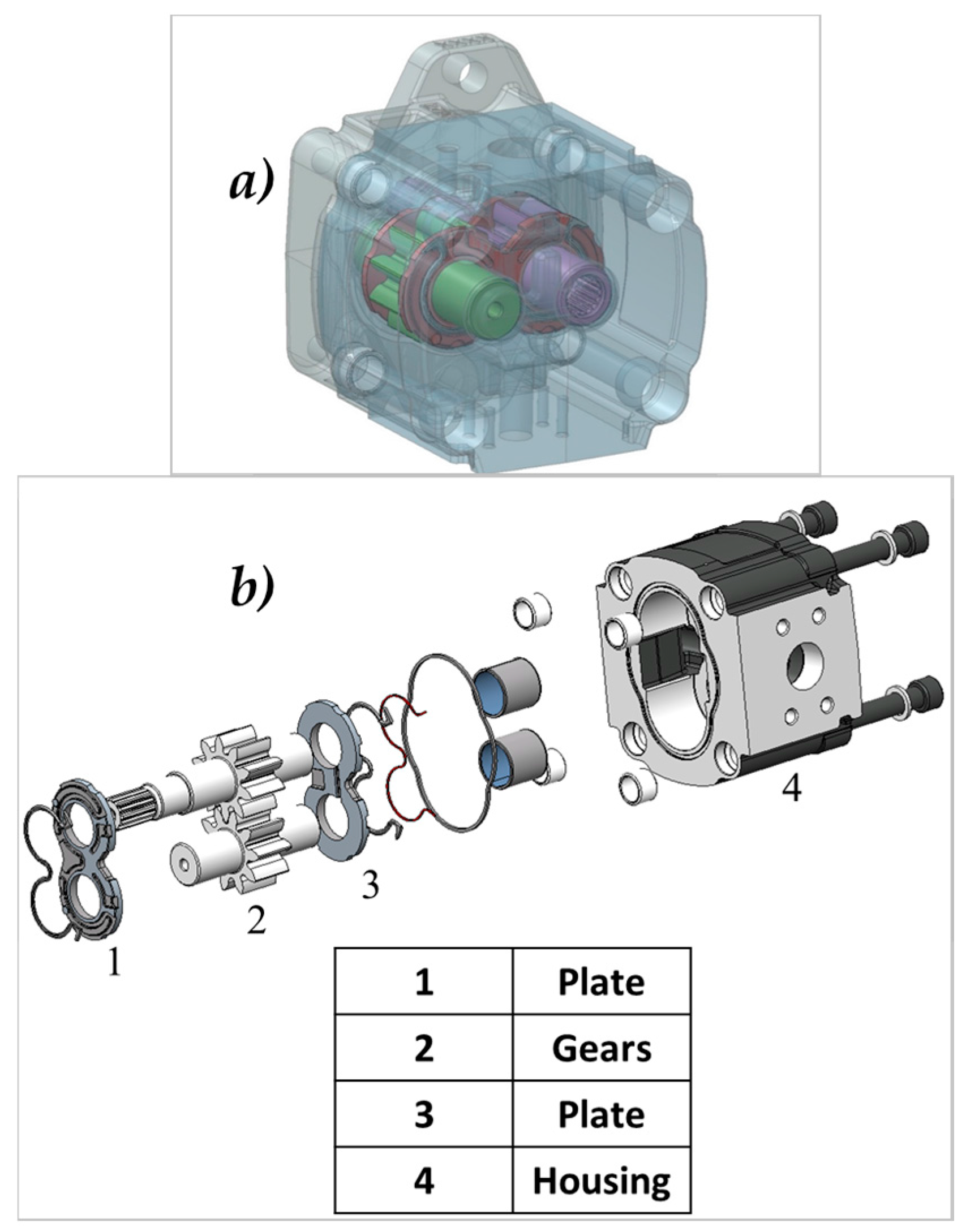
Figure 2.
Grooves inside the lateral plates.
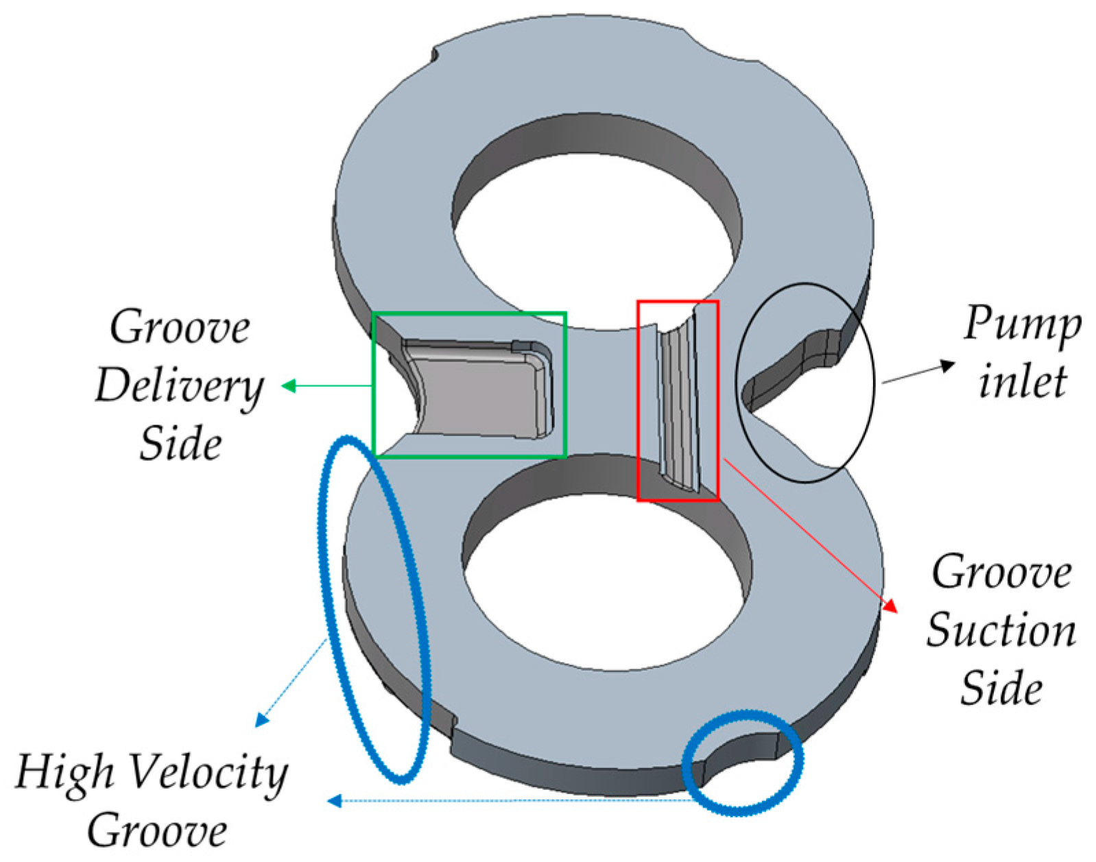
Figure 3.
Extracted fluid volume of the external gear pump, (a) entire fluid volume; (b) fluid volume of the plate; (c) fluid volume in rotation; (d) fluid volume of the ports.
Figure 3.
Extracted fluid volume of the external gear pump, (a) entire fluid volume; (b) fluid volume of the plate; (c) fluid volume in rotation; (d) fluid volume of the ports.

Figure 4.
(a) Binary tree mesh; (b) mismatched grid interface (MGI) between volumes.
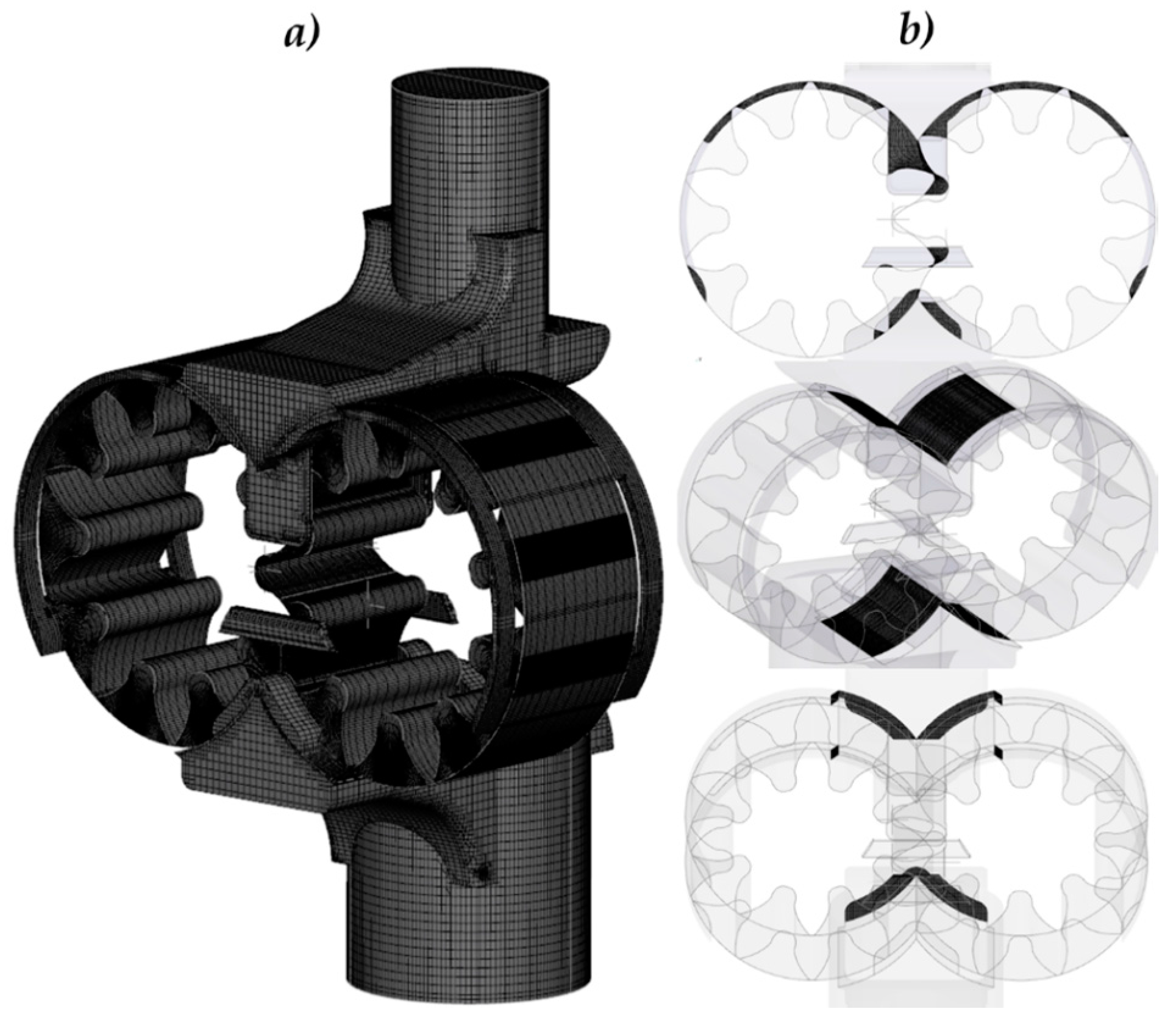
Figure 5.
Mesh of the rotating fluid volume and size of the minimum gaps.

Figure 6.
Front view of the gears; angle θ and φ.

Figure 7.
Three different pump configurations: (a) φ of −0.10° and gap size of 71.8 μm; (b) φ of −0.17° and gap size of 45.9 μm and (c) φ of −0.28° and gap size of 5.3 μm.
Figure 7.
Three different pump configurations: (a) φ of −0.10° and gap size of 71.8 μm; (b) φ of −0.17° and gap size of 45.9 μm and (c) φ of −0.28° and gap size of 5.3 μm.
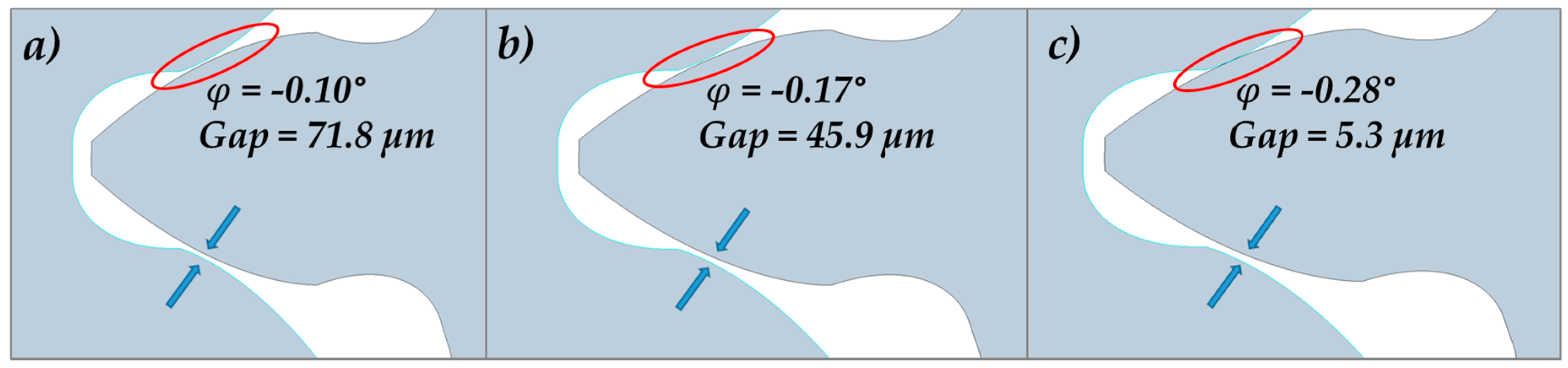
Figure 8.
Mesh sensitivity—flow-rate vs cells number at 1500 rpm and a delivery pressure of 50 bar.

Figure 9.
(a) Pressure, velocity and vapor mass fraction—residual drop analysis Ri; (b) error on the mass flow vs residual drop Ri.
Figure 9.
(a) Pressure, velocity and vapor mass fraction—residual drop analysis Ri; (b) error on the mass flow vs residual drop Ri.

Figure 10.
(a) Test bench of Casappa S.p.A.; (b) test bench layout.
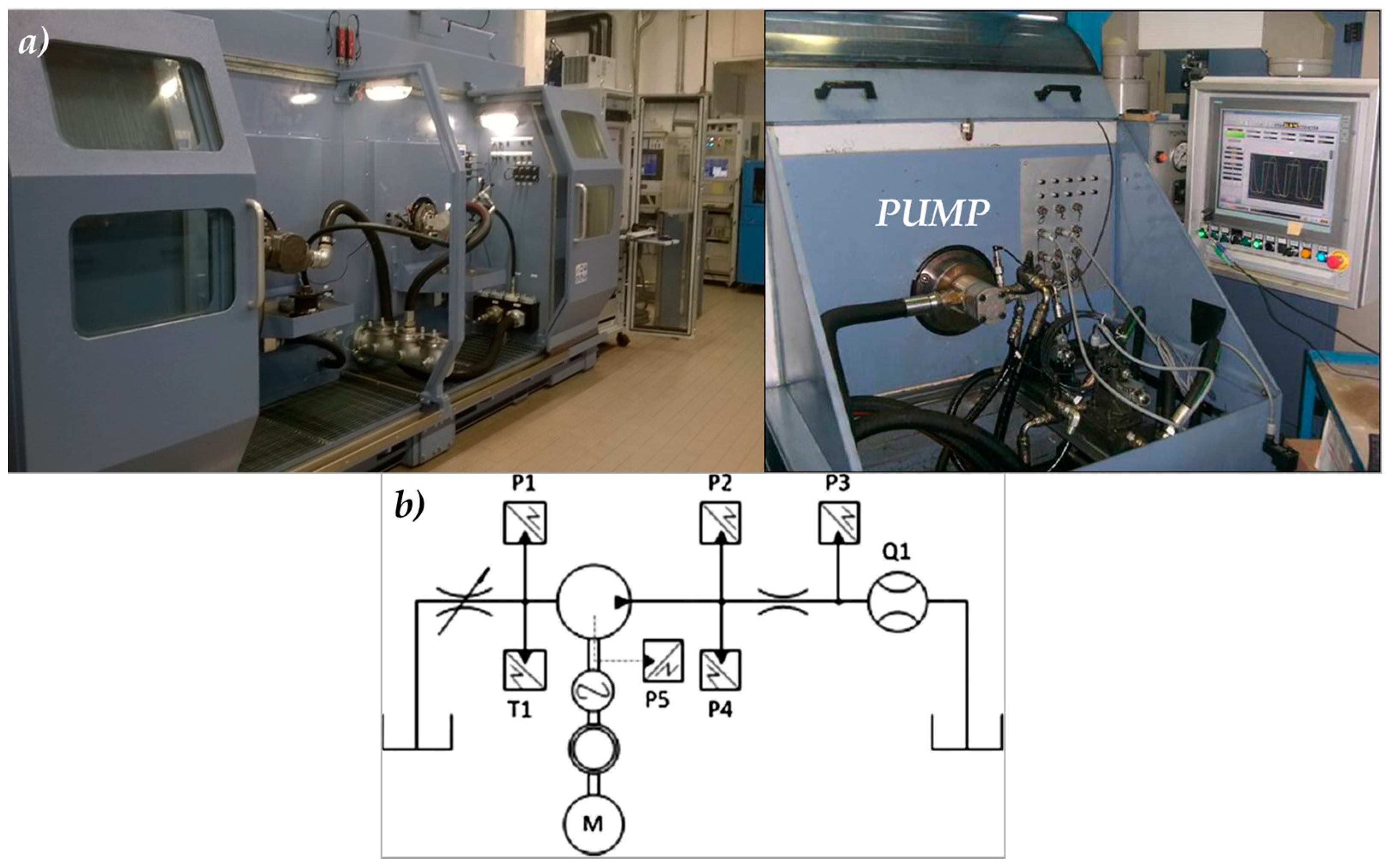
Figure 11.
Absorbed torque—comparison between model and experimental data. (a) 1000 rpm; (b) 1500 rpm and (c) 2500 rpm.
Figure 11.
Absorbed torque—comparison between model and experimental data. (a) 1000 rpm; (b) 1500 rpm and (c) 2500 rpm.

Figure 12.
Delta torque between experimental data and simulation data at 1000, 1500 and 2500 rpm.
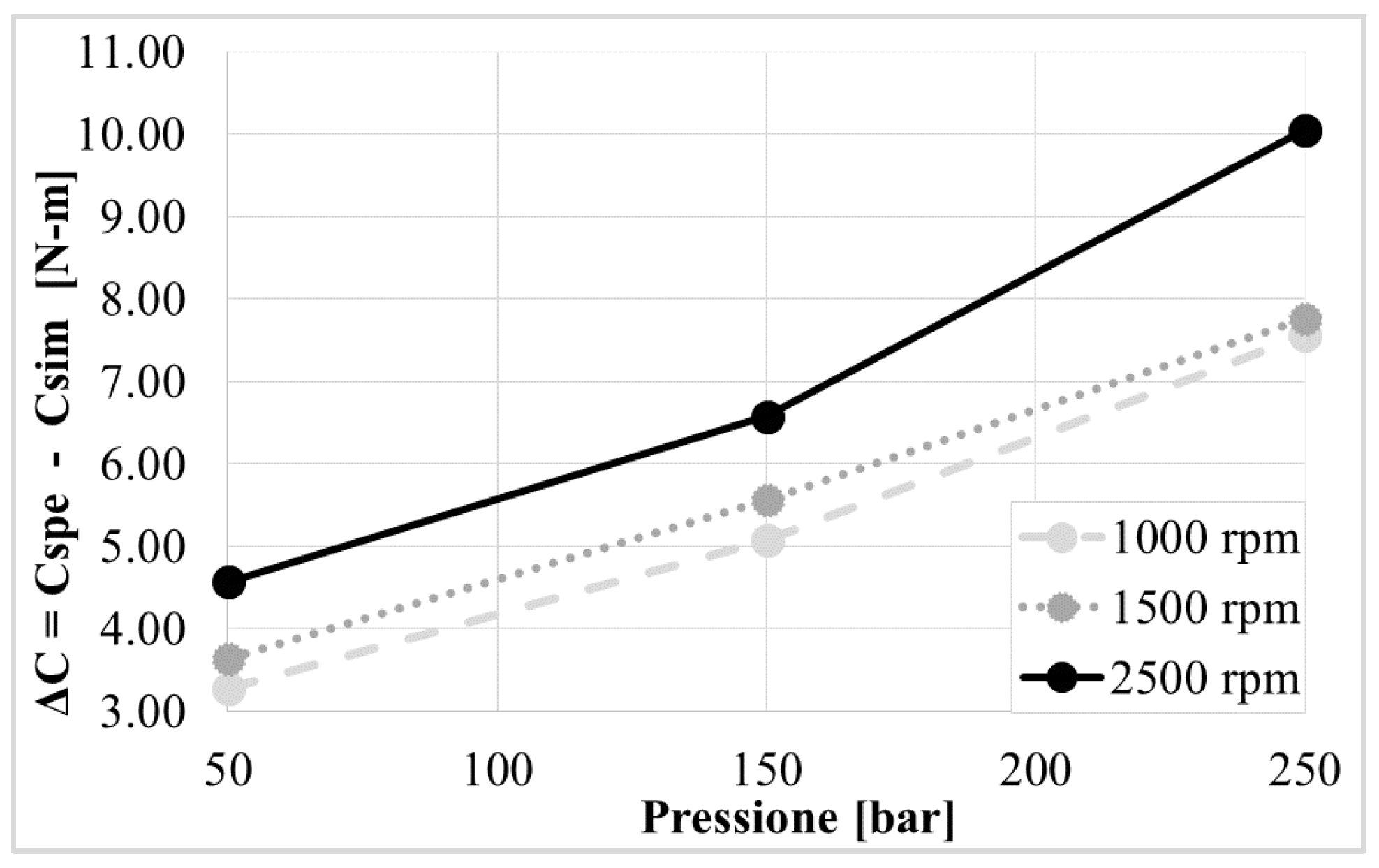
Figure 13.
Pressure vs. delivery flow-rate comparison at 50 and 80 °C.

Figure 14.
Velocity magnitude at (a) 50 °C; (b) 80 °C and (c) zoomed area.
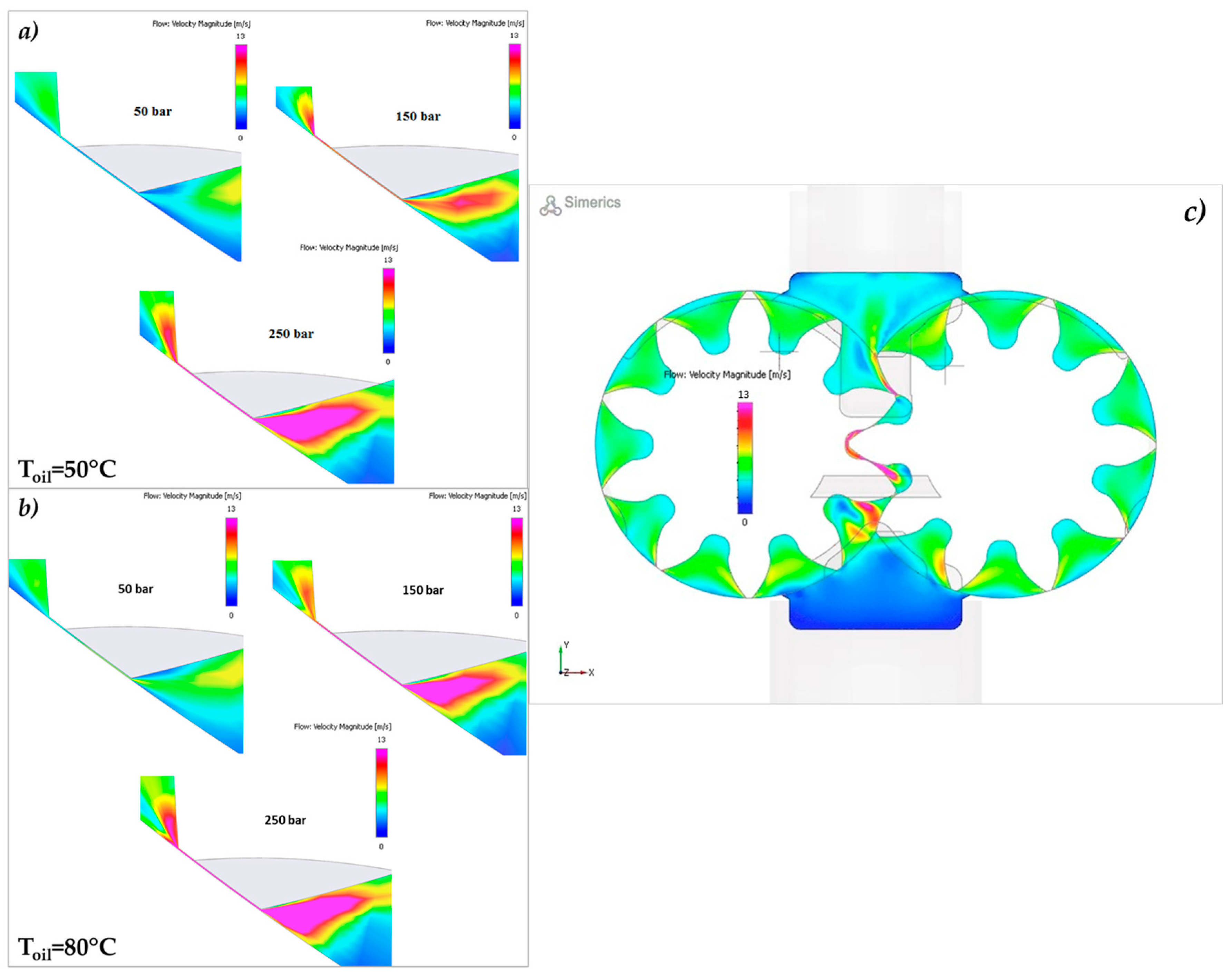
Figure 15.
Pressure evolutions for two pressure levels at Toil of 50 °C.
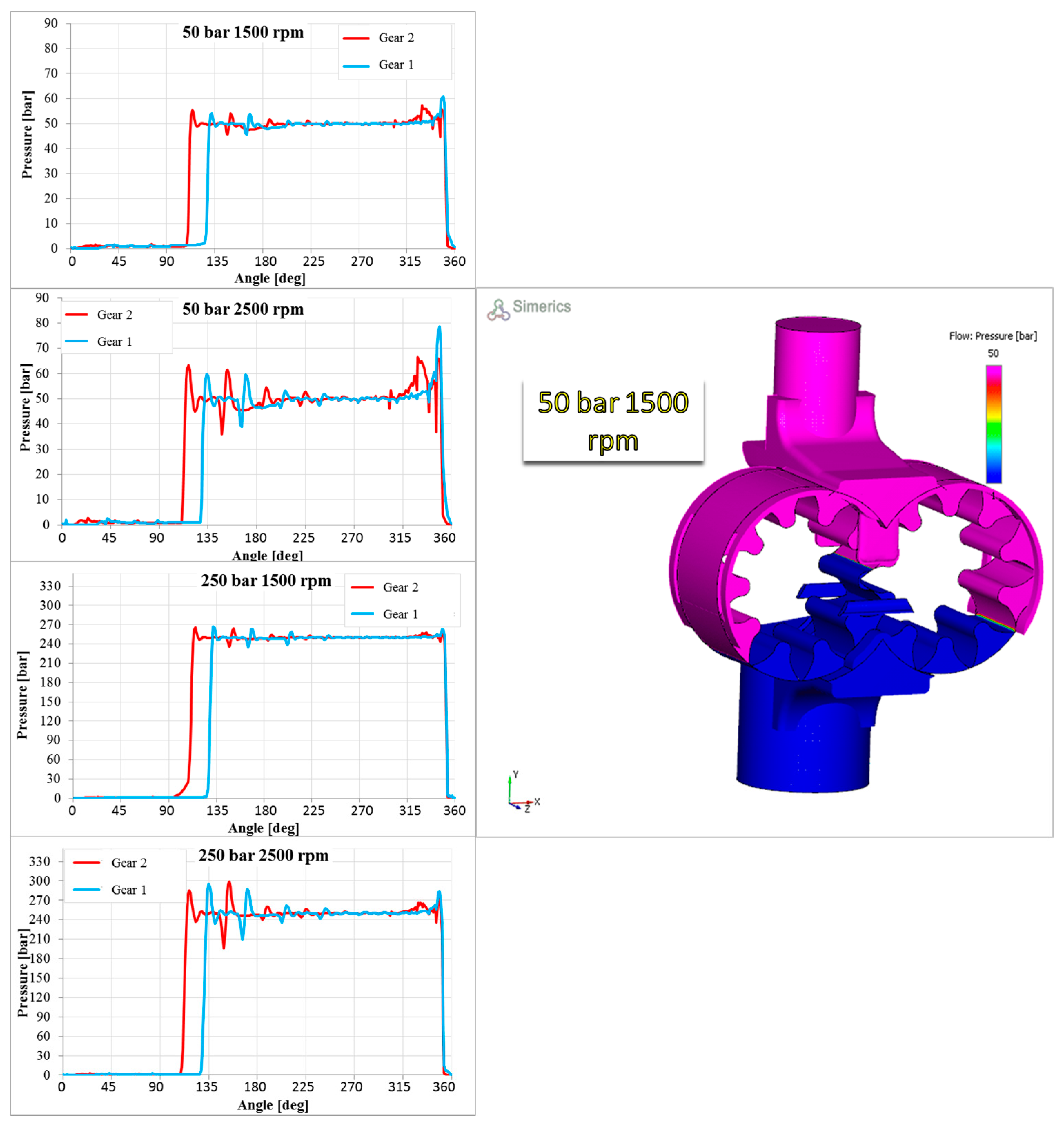
Figure 16.
Pressure evolutions for two pressure levels in the range 0–3.5 bar, at Toil of 50 °C.

Figure 17.
(a) Calibrated orifice geometry, (b) pressure ripples monitoring point; (c) mesh of the entire model.
Figure 17.
(a) Calibrated orifice geometry, (b) pressure ripples monitoring point; (c) mesh of the entire model.

Figure 18.
Pressure ripple comparison at 50 bar and 150 bar, 2500 rpm and 50 °C.

Figure 19.
Distribution of the total gas fraction in a section view of the pump at 250 bar, 2500 rpm and 50 °C for a shaft rotation of θ = 9°, 18°, 27° and 36°.
Figure 19.
Distribution of the total gas fraction in a section view of the pump at 250 bar, 2500 rpm and 50 °C for a shaft rotation of θ = 9°, 18°, 27° and 36°.

Figure 20.
Total gas fraction behaviors at 1500 and 2500 rpm.

Table 1.
Pump main features—Casappa KP30.
| Pump Main Features | Value |
|---|---|
| Nominal displacement | 44 cm3 |
| Inlet pressure range | 0.7–3 bar |
| Max. continuous pressure | P1 = 250 bar |
| Max. intermitted pressure | P2 = 270 bar |
| Max. peak pressure | P3 = 290 bar |
| Rotational speed | Min = 350 min−1 Max = 3000 min−1 |
Table 2.
Mesh sensitivity varying the mesh size in the boundary layers, simulations at 1500 rpm.
| Delivery Pressure | ΔQ% Mesh 1 | ΔQ% Mesh 2 |
|---|---|---|
| pdelivery = 50 bar | 0.72% | 0.24% |
| pdelivery = 200 bar | 1.78% | 1.36% |
© 2017 by the authors. Licensee MDPI, Basel, Switzerland. This article is an open access article distributed under the terms and conditions of the Creative Commons Attribution (CC BY) license (http://creativecommons.org/licenses/by/4.0/).
Share and Cite
MDPI and ACS Style
Frosina, E.; Senatore, A.; Rigosi, M. Study of a High-Pressure External Gear Pump with a Computational Fluid Dynamic Modeling Approach. Energies 2017, 10, 1113. https://doi.org/10.3390/en10081113
AMA Style
Frosina E, Senatore A, Rigosi M. Study of a High-Pressure External Gear Pump with a Computational Fluid Dynamic Modeling Approach. Energies. 2017; 10(8):1113. https://doi.org/10.3390/en10081113
Chicago/Turabian StyleFrosina, Emma, Adolfo Senatore, and Manuel Rigosi. 2017. "Study of a High-Pressure External Gear Pump with a Computational Fluid Dynamic Modeling Approach" Energies 10, no. 8: 1113. https://doi.org/10.3390/en10081113
Note that from the first issue of 2016, this journal uses article numbers instead of page numbers. See further details here.