Wave Energy Resource Assessment off the Coast of China around the Zhoushan Islands
by
Yong Wan
1,2,3,*, 
Chenqing Fan
2,
Jie Zhang
2,
Junmin Meng
2,
Yongshou Dai
1,
Ligang Li
1,
Weifeng Sun
1,
Peng Zhou
1,
Jing Wang
3 and
Xudong Zhang
3 1
College of Information and Control Engineering, China University of Petroleum, No. 66, Changjiangxi Road, Huangdao District, Qingdao 266580, China
2
The First Institute of Oceanography, State Oceanic Administration, No. 6, Xianxialing Road, Laoshan District, Qingdao 266061, China
3
College of Information Science and Engineering, Ocean University of China, No. 238, Songling Road, Laoshan District, Qingdao 266100, China
*
Author to whom correspondence should be addressed.
Energies 2017, 10(9), 1320; https://doi.org/10.3390/en10091320
Submission received: 26 July 2017
/
Revised: 21 August 2017
/
Accepted: 29 August 2017
/
Published: 1 September 2017
(This article belongs to the Section L: Energy Sources)
Abstract
:Based on ERA-Interim reanalysis wave field data for the 36 years from 1979 to 2014, the temporal and spatial distributions and development potential of wave energy are studied in detail in the offshore and relatively nearshore waters adjacent to the Zhoushan Islands. The results show that areas of relatively high wave energy are located in the offshore waters to the east and southeast of the Zhoushan Islands. The potential wave energy in relatively nearshore waters (water depths from 10 m to 65 m) is relatively higher and especially in the nearshore waters to the southeast of the city of Taizhou, Zhejiang Province, which are suitable locations for wave energy development. The conclusions provide scientific guidance for wave energy development in the sea areas adjacent to the Zhoushan Islands.
1. Introduction
Ongoing social and economic development is increasing the demand for energy. The energy supply problems arising from a shortage of conventional fossil energy and the pollution problems resulting from the overuse of conventional fossil energy are intensifying. Wave energy is a type of clean and renewable energy that does not produce carbon dioxide. The development of wave energy can effectively ease the energy crisis and environmental pollution, but before the development of wave energy, the reserves and the temporal and spatial distributions of wave energy in interesting areas must be reliably assessed. Many wave energy assessment studies have been conducted in different countries with respect to global sea areas and large-scale sea areas in different regions. Cornett [1] investigated global wave energy resources based on a third-generation model, Wave Watch III (WAVEWATCH-III). Barstow et al. [2] and Mork et al. [3] assessed the wave energy potential of global oceans from deep waters to relatively nearshore waters based on the global wave dataset Worldwaves. Arinaga and Cheung [4] employed 10 years of wave field data from WAVEWATCH-III to evaluate the global wave energy. Zheng et al. [5] evaluated the wind wave energy and swell energy for global oceans in detail based on global wind wave fields and swell fields from European Centre for Medium-Range Weather Forecasts (ECMWF) ERA-40 reanalysis data over the last 45 years. Pontes et al. [6] and Pontes [7] evaluated the wave energy in Europe’s coastal waters in the Atlantic and Mediterranean by using the wave model Wave Modelling project (WAM). Soares et al. [8] assessed the wave energy in detail along the Atlantic European coast by using WAVEWATCH-III and Simulating Waves Nearshore (SWAN). Henfridsson et al. [9] studied the wave energy potential of the Baltic Sea based on a hindcast dataset. Zheng et al. [10] and Zheng et al. [11] comprehensively and systematically assessed the wave energy resources in the China Sea by using high-resolution wave field data that were simulated by the WAVEWATCH-III wave model and obtained the reserves and distribution of the wave energy in a large-scale area in the China Sea. Zheng et al. [12] and Zheng et al. [13] analyzed the wind energy in the global ocean and the wave energy in the China Sea in detail based on Cross Calibrated Multi-Platform (CCMP) wind data and WAVEWATCH-III wave data. Wave energy and wind energy assessments in large-scale areas are essential to understand the temporal and spatial distributions of wave energy and can provide macroscopic references for decision makers to evaluate wave energy projects. However, for practical engineering applications, wave energy assessments in large-scale areas cannot meet the requirements for the siting of wave farms and the design of wave energy converters (WECs). Some wave energy assessments in relatively nearshore, small-scale sea areas were carried out for siting wave farms. Kim et al. [14] assessed the wave energy in offshore deep waters in the sea areas adjacent to Korea based on a hindcast dataset from 1979 to 2003 and evaluated the wave energy in the relatively nearshore waters of Hongdo by using the SWAN model. From 2009 to 2011, Iglesias et al. [15,16,17,18,19,20] conducted a refined evaluation of several small-scale areas in the sea areas adjacent to Spain based on wave model data. Liang et al. [21] assessed the wave energy for two important areas in the adjacent seas to the east of China based with 22 years of wave data by using the SWAN model. Zheng et al. [22] assessed the wave energy in key locations along the relatively nearshore coastline waters of Taiwan based on buoy data from adjacent sea areas in 12 regions of Taiwan. The above works provide good references for wave energy assessment in relatively nearshore, small-scale sea areas.
The region of interest in this study is the sea area adjacent to the Zhoushan Islands, which is shown in Figure 1 (rectangular region in green). The Zhoushan Islands, located in the East China Sea, are the largest islands in China and constitute 20% of the country’s islands, with 1390 islands and a population of one million. Fish production is important in the sea areas adjacent to the Zhoushan Islands. In this area, the demand for energy is enormous because of the power that is required by residents and for fish production and sea water desalination. Wave energy is exploitable in the sea areas adjacent to the Zhoushan Islands. Reasonable wave energy development could provide a sustainable energy supply for the development of the Zhoushan Islands and its adjacent regions, however, a comprehensive understanding of the development value of wave energy in the sea areas adjacent to the Zhoushan Islands is lacking. Therefore, based on high-resolution and high-accuracy ERA-Interim reanalysis wave field data from the ECMWF from 1979 to 2014, the temporal and spatial distributions and the development potential of wave energy are studied in the sea areas adjacent to the Zhoushan Islands. The conclusions can provide reliable references for practical engineering applications, such as siting wave farms and the design and operation of WECs in the sea areas adjacent to the Zhoushan Islands.
In the remainder of this paper, the data and their verification are described in Section 2. In Section 3, the distributions of the wave energy are analyzed in the offshore, large-scale areas of these sea areas to help readers understand the overall distribution of the wave energy in the sea areas adjacent to the Zhoushan Islands. In Section 4, we establish a novel criterion for the regional division of wave energy that is suitable for local sea areas and identify the best regions for wave energy in the relatively nearshore waters of the Zhoushan Islands with a focus on relatively nearshore applications. In Section 5, key single locations are selected in key regions, for which the wave energy is analyzed in detail, and important reference information for the practical development of wave energy is described. The last section provides the conclusions.
2. Data and Their Verification
The significant wave height (Hs, m) and the energy period (Te, s) are two basic parameters for calculating the characteristic quantity of wave energy. The energy period is a mean wave period that can be calculated by m−1/m0 which are spectral moments of the wave spectrum and is related to energy [23]. The wave data in this paper were ERA-Interim reanalysis wave field data over the last 36 years, which were collected by ECMWF with a spatial resolution of 0.125 × 0.125 and a temporal resolution of 6 h. The ECMWF is one of the main data reanalysis centers in the world. The ERA-Interim reanalysis data and its previous edition, ERA-40, have been widely used [5,24,25]. The accuracy of wave energy assessment is directly related to the accuracy of the wave parameters, so we verified the accuracy of the ERA-Interim wave field data based on data from two buoys located in the area of interest. The buoys were Directional Waverider MkIII buoys from Datawell BV (Haarlem, The Netherlands). Directional Waverider buoys are the most advanced buoys available worldwide and dominate the international market for wave buoys. The wave data that were measured by these buoys were averaged values from 10 min of spectral data and were calculated from the spectral moment.
The locations of the buoys are shown in Figure 2, and the specifications of the buoys are shown in Table 1. The locations and observation times of the buoys were different from the ERA-Interim data, so the ERA-Interim data, which were gridded data, were interpolated in space and time to collocate with the buoy data. The spatial resolution and the temporal resolution of the ERA-Interim data were 0.125 × 0.125 and 6 h, respectively, and the locations and observation times of the buoys were fixed values. First, the 4 gridded ERA-Interim point data closest to the buoy were interpolated according to the longitude and latitude of the buoy by using bilinear interpolation to obtain collocated ERA-Interim data at the buoy location, achieving interpolation in space. Then, the ERA-Interim data at the 2 closest times to the observation time of the buoy were interpolated by using linear interpolation to obtain collocated ERA-Interim data at the observation time of the buoy, achieving interpolation in time. The two parameters Hs and Te, were verified; the results are shown in Figure 3, and the error indices are shown in Table 2. The root mean square error (RMSE) and the correlation coefficient (CC) can be calculated as follows:
where denotes the wave parameters from the buoys; denotes the wave parameters from the ERA-Interim; and denote the mean value of the wave parameters from the buoys and the ERA-Interim respectively; and is the number of samples. The units of measurement of the RMSE were meters and seconds for Hs and Te, respectively. The correlation coefficient is a statistical index to reflect the close degree of correlation between wave parameters from the buoys and those from the ERA-Interim. The RMSE of Hs for buoy 006 was 0.31 m and the CC was 0.90; the RMSE for Te was 0.56 s and the CC was 0.78. The RMSE of Hs for buoy kzszs was 0.36 m and the CC was 0.78; the RMSE for Te was 0.81 s and the CC was 0.70. The results show that the wave field data from the ERA-Interim were accurate in the sea areas adjacent to the Zhoushan Islands and are suitable for wave energy assessment.
3. Wave Energy Analysis in Offshore Waters
Indices such as the distributions of the significant wave height, energy period, wave power density, Pw (kW/m) and stability of the wave energy (ST) were employed to analyze the temporal and spatial distributions of the wave climate and wave energy in the offshore large-scale areas in the sea areas adjacent to the Zhoushan Islands and can provide macroscopic references for wave energy development.
3.1. Temporal and Spatial Distributions of the Wave Climate
Before assessing the wave energy, researchers always analyze the wave climate distribution of the area of interest and to better understand the distribution of the wave energy resources [4,26]. Therefore, we analyze the distributions of the significant wave height and energy period in detail based on the ERA-Interim data from 1979 to 2014.
3.1.1. Temporal and Spatial Distributions of the Significant Wave Height
Figure 4 shows the annual average and seasonal average distributions of Hs in the sea areas adjacent to the Zhoushan Islands, which were calculated based on the ERA-Interim data from 1979 to 2014. The results show that the annual average Hs (approximately 0.7–1.6 m) gradually decreased from the offshore deep water areas to the relatively nearshore shallow water areas, which is the direction in which the waves are travelling. Areas with large annual average Hs values (approximately 1.4–1.6 m) were primarily located in the eastern and southeastern offshore sea waters of the Zhoushan Islands, where the sea-states are higher. Areas with small annual average Hs values (below 0.7 m) were primarily located in the relatively nearshore waters of the Changjiang Estuary and Hangzhou Bay, where the sea-states were lower. In this area, the seasons are influenced by the East Asian monsoon climate and extreme sea conditions from the ocean. Winter is from December to February; spring is from March to May; summer is from June to August; and autumn is from September to November. The average Hs showed pronounced seasonal variations in the sea areas adjacent to the Zhoushan Islands. Hs was higher during autumn and winter than during spring and summer because of the monsoon. The sea-states were highest during winter, when Hs reached 2 m; this value was slightly lower during autumn. Hs had similar values during spring and summer.
3.1.2. Temporal and Spatial Distributions of the Energy Period
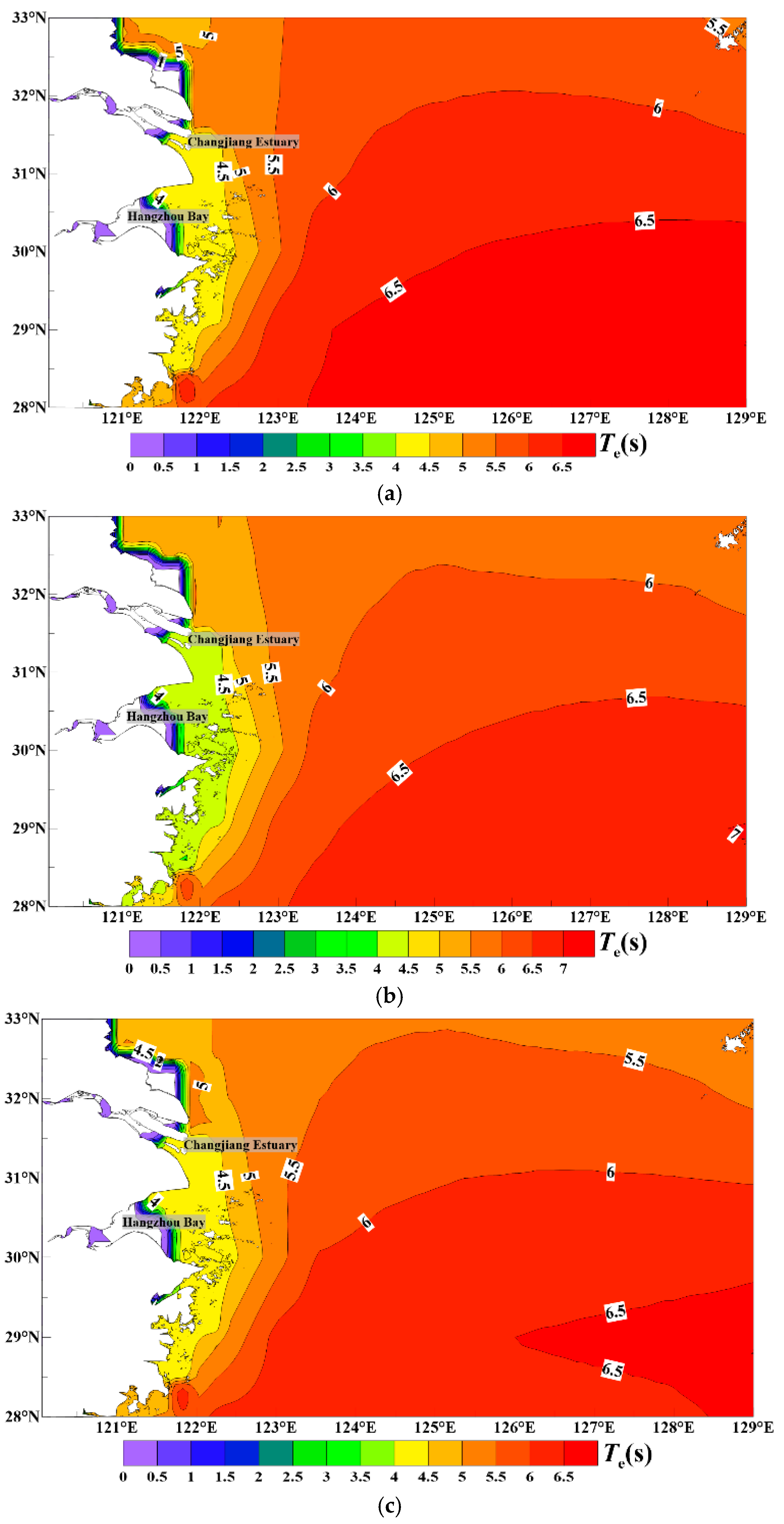
Figure 5 shows the annual average and seasonal average distributions of Te in the sea areas adjacent to the Zhoushan Islands, which were calculated based on the ERA-Interim data from 1979 to 2014. The results show that the annual average Te values were relatively small (approximately 4.0–5.5 s) in the relatively nearshore waters and were relatively large (approximately 5.5–6.5 s) in the offshore waters. Te was steady in most of the sea areas. The results of the seasonal average show that the seasonal variation in Te was not obvious: Te was approximately 5.5–7.0 s in most of the sea areas and was slightly higher during winter and autumn. The seasonal spatial distributions of Te were similar to the annual average distributions. A relatively steady Te is advantageous for wave energy stability.
3.2. Calculation Method for the Wave Power Density
The wave power density (Pw) is the most important index for wave energy assessment and is related to the accuracy of the wave energy assessment. The water depth is shallow in the sea areas adjacent to the Zhoushan Islands. The influence of the water depth must be considered when calculating Pw to improve the accuracy of Pw because of shoaling. In this paper, we considered the influence of the water depth when calculating Pw. The wave power density for all water depths can be calculated as follows [27]:
where is the wave energy density (J/m2), is the density of sea water (kg/m3), g is the acceleration from gravity (m/s2), is the wavenumber (m−1), is the wavelength (m), d is the water depth (m), and .
The bathymetry data were obtained from the University of California San Diego (UCSD) website and had a spatial resolution of 1′ × 1′ [28]. refers to the average wavelength according to the wave number and is estimated by using the mean wave period; to obtain accurate results, was calculated according to a relationship that was presented by Wen et al. [29], which was obtained by experimentation. can be calculated as follows:
In deep water, the wave power density can often be calculated as follows:
3.3. Temporal and Spatial Distributions of the Wave Power Density
The annual average and seasonal average distributions of Pw in the sea areas adjacent to the Zhoushan Islands, which were calculated based on the ERA-Interim data from 1979 to 2014, are shown in Figure 6. According to the results of the annual average, Pw (approximately 2–13 kW/m) gradually decreased from the offshore deep water areas to the relatively nearshore shallow water areas because the wave power declines as the resource moves into shallow water. Areas with relatively large annual average Pw values (approximately 10–13 kW/m) were primarily located in the eastern and southeastern offshore sea waters of the Zhoushan Islands, where wave energy was relatively abundant. Areas with small annual average Pw values (below 2 kW/m) were primarily located in the relatively nearshore waters of the Changjiang Estuary and Hangzhou Bay, where the development value of wave energy was low. It is very important to note that compared with global sea areas [31], the Zhoushan Islands coastal average wave energy resource is weak as it only reaches 10 kW/m nowhere along the coastline, the wave resource investigated here is weak in comparison to the global resource. So we declare the results discussed in this paper only aim at local sea areas around the Zhoushan Islands and want to provide references for wave farm construction and siting in this local areas. All conclusions in the next sections about abundant level of wave energy are relative to local sea areas around the Zhoushan Islands not relative to global scale. Pronounced seasonal variations in the wave energy were present in the sea areas adjacent to the Zhoushan Islands because of the East Asian monsoon climate and extreme sea conditions from the ocean. Pw was higher during autumn and winter than during spring and summer because of this monsoon climate. Wave energy was most abundant in winter, when Pw reached 18 kW/m. Pw was slightly lower during autumn than during winter. Spring and summer had similar Pw values, although Pw was slightly higher during summer, when typhoons from the West Pacific influence this area. Wave energy was usable, and has certain development value in the sea areas adjacent to the Zhoushan Islands, with autumn and winter being the key periods for energy extraction.
3.4. Stability of Wave Energy
Several studies have shown that we also must consider the stability when assessing wave energy resources. The stability of wave energy means that the wave energy is sustainable for a long time and the variation in the wave energy is small. Abundant and stable wave energy is advantageous for exploitation and utilization [1]. Therefore, studying the stability of the wave energy in areas of interest is important. The stability index (ST) can express the stability of wave energy and can be calculated as follows [24]:
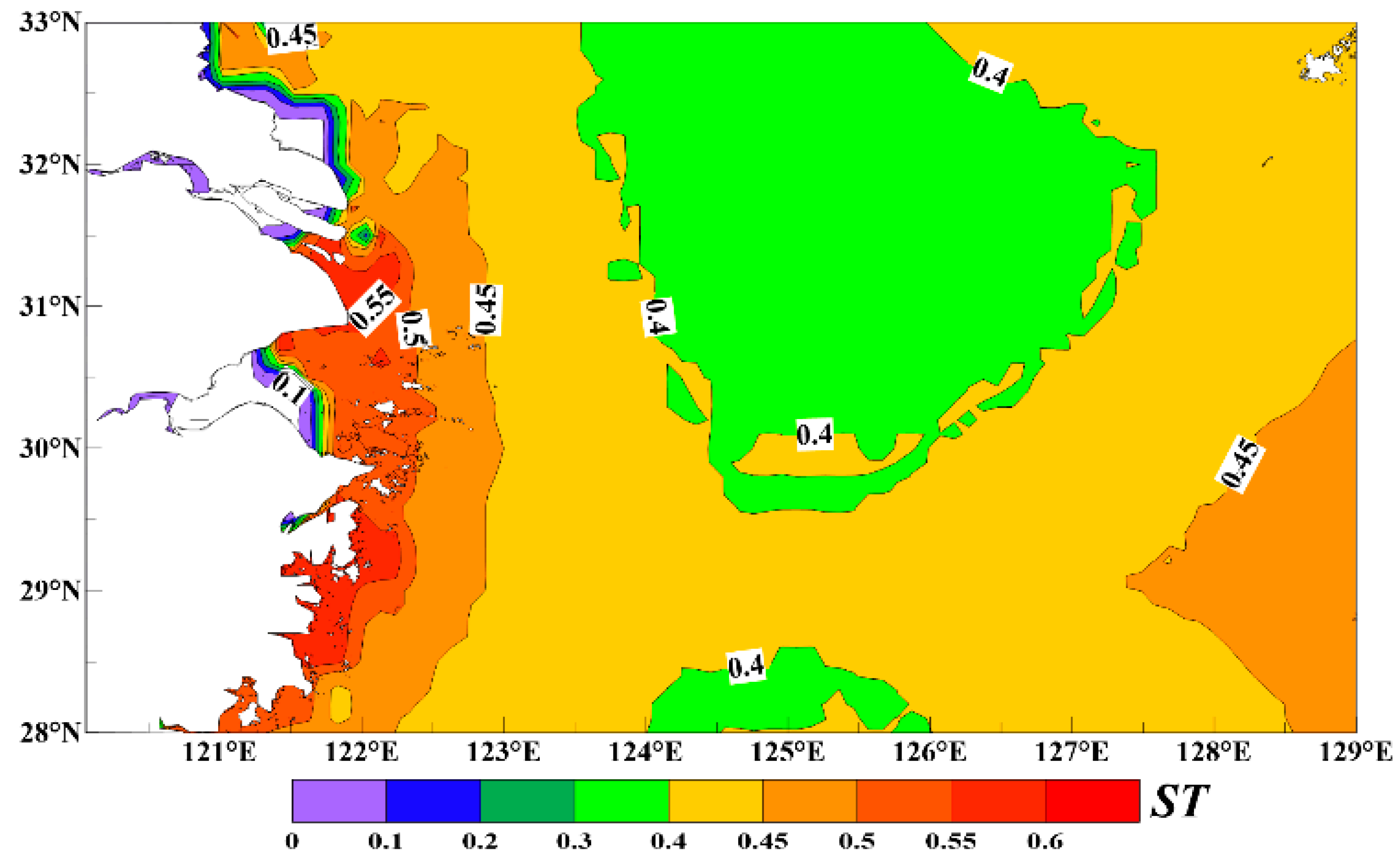
where is the mean wave power density in the minimum energy month (kW/m) and is the annual mean wave power density over the last 36 years (kW/m). Equation (6) shows that the mean wave power density in the minimum energy month is closer to the annual mean wave power density when ST is higher, indicating less variation in the wave power density. Under this circumstance, the wave energy is more stable and sustainable. Figure 7 shows the distributions of ST in the sea areas adjacent to the Zhoushan Islands, which were calculated based on ERA-Interim data over the last 36 years. This figure shows that the stability was relatively higher along relatively nearshore coastline areas, with the ST values all above 0.45; the stability was relatively lower in offshore sea areas, with the ST values are below 0.45. The stability further decreased in the sea areas to the east of the Zhoushan Islands, with the ST values below 0.40 because of the influence of tropical storms from the ocean. A stable area of wave energy that was sheltered from the Ryukyu Islands was present to the northwest of the Ryukyu Islands, with ST values above 0.45. Overall, the stability in relatively nearshore waters that are suitable for wave energy development was relatively good, which is advantageous for wave energy development.
3.5. Discussion on Wave Energy in Offshore Waters
In Section 3, we analyzed the characteristics of the wave energy in the offshore waters in the sea areas adjacent to the Zhoushan Islands in detail. The results showed that wave energy is relatively weak in the sea areas adjacent to the Zhoushan Islands compared with global ocean, for the most part less than 10 kW/m annually. Although the wave energy is not abundant, it is usable and has certain potential for development. In the sea areas around the Zhoushan Islands, the areas with relatively high annual average wave power density (approximately 10–13 kW/m) are primarily located in the eastern and southeastern offshore sea waters of the Zhoushan Islands. The wave power density is higher during autumn and winter than during spring and summer because of the monsoon climate. Autumn and winter are the key periods for energy extraction. In addition, the wave energy is relatively more stable and sustainable in the relatively nearshore waters than in the offshore waters. However, the relatively nearshore waters have less wave energy than the offshore waters. The utilization and development of wave energy are mainly located in relatively nearshore waters because of the current limits of technology and the costs of wave farms. Therefore, the relatively nearshore sea areas to the east of the Zhoushan Islands, which have an annual average wave power density of 5–8 kW/m and a stability index of 0.4–0.45, are the most suitable areas for wave energy development in this areas.
4. Division of Key Wave Energy Regions in Relatively Nearshore Waters
At present, the development of wave energy is mainly located in relatively nearshore local regions because of the technological limits and the cost of development. Accurately evaluating wave energy in relatively nearshore local regions is very important to support practical engineering in the development of wave energy. A single location mode is usually adopted in relatively nearshore wave energy assessment. That is, we can select locations (fixed locations) in relatively nearshore waters and study the distributions of the wave energy in each location. Before selecting key single locations in relatively nearshore waters, we must first carry out a regional division for wave energy in relatively nearshore waters and identify key regions of wave energy. Then, we can select key locations for studies in these regions.
4.1. Division Criterion
A novel criterion for regional division that is suitable for local sea areas was established. This criterion is based on three parameters: the annual average wave power density (Pw, kW/m), annual average effective time (, h) and total wave energy (TWE, J). The annual average effective time is the annual average duration for the wave energy, with 1 m ≤ Hs ≤ 4 m. The reason is wave energy converters will possibly be damaged and have higher cost for maintenance in high sea states, for example Wave Star will operate in storm protection mode and stop generating power when significant wave height is above 3.0 m [32]. At the same time, when significant wave height is less than 1 m, it may not be possible to economically harvest energy with present state WECs. The total wave energy can be calculated by using two main methods: the synoptic method and climatology method [33,34]. The climatology method is the better choice because it uses a long-term average, which can represent a long-term trend. The regional division criterion is established as follows:
- (1)
- Nine small continuous areas that were 0.5 × 0.5 in size were selected in the relatively nearshore waters of the Zhoushan Islands, which are shown in Figure 8. First, the annual average Pw and annual average TE of every grid were calculated for each small area. Then, the results of every grid in each small area were averaged, providing the annual average Pw and the annual average TE of each small area. Finally, the TWE for each small area was calculated.
- (2)
- The comprehensive division coefficient (CDC) was defined as follows:When the CDC is higher, wave energy is abundant and the potential of development is higher.
- (3)
- Five grades were established according to the CDC. The general criterion of the regional division is shown in Table 3. The potential of the wave energy increases from levels 1 to 5, which indicate poor, available, good, better and best potential. The ranges of each index in Table 3 exhibit different value ranges for the different areas. The threshold value a-c can be determined by equal division as follows (with as an example):Then:where is the maximum annual average and is the minimum annual average .The method for determining the other threshold values is similar to that of .
- (4)
- Thresholds were calculated for each index, as shown in Table 4.
- (5)
- The criterion of the regional division was established. This criterion is suitable for the relatively nearshore waters of the Zhoushan Islands. The results are shown in Table 5.
4.2. Division Results
We calculated the CDC and performed a regional division for nine small areas with a size of 0.5 × 0.5 in the relatively nearshore waters of the Zhoushan Islands according to the regional division criterion in Section 4.1; the results are shown in Figure 8. This figure shows that the grade of area A4 was one (CDC of 3518), showing poor development potential. The grades of areas A1 and A8 were two (CDCs of 12,400 and 9901, respectively), showing available development potential. The grades of areas A2, A3 and A7 were three (CDCs of 23,213, 16,324 and 18,697, respectively), showing good development potential. The grades of areas A5, A6 and A9 were five (CDCs of 54,187, 54,342 and 54,084, respectively), showing the best development potential. In this paper, we selected areas A5, A6 and A9 as the key areas for wave energy development in these relatively nearshore waters.
5. Wave Energy Analysis in the Key Locations in the Relatively Nearshore Waters
We selected key locations after determining the key areas. Indices that involved siting wave farms and the design of WECs were analyzed to provide reliable references for engineering in the development of wave energy in relatively nearshore waters.
5.1. Selecting Key Locations in the Relatively Nearshore Waters
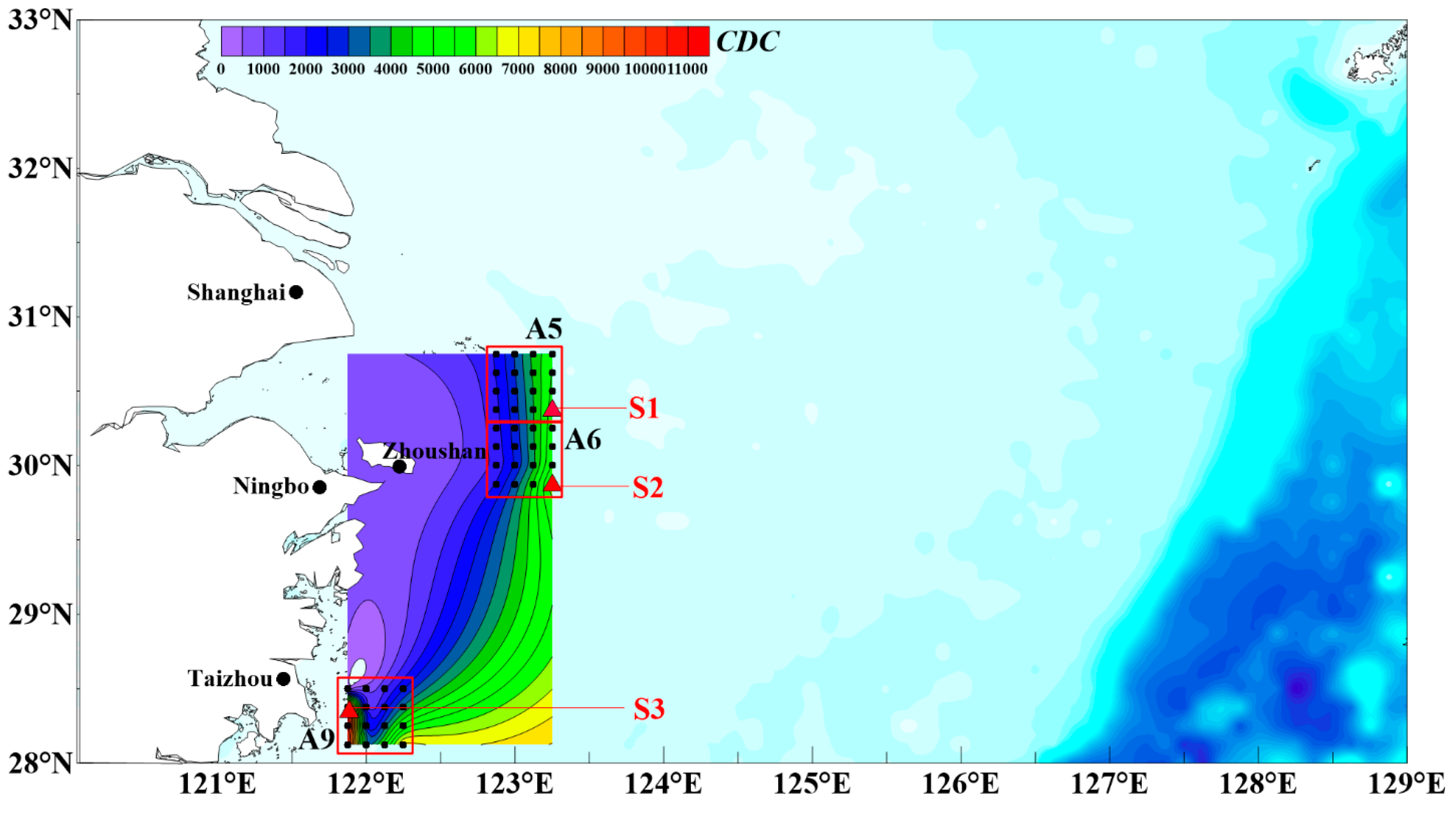
We referred to the CDC in Section 4.1 when selecting key locations in these relatively nearshore waters and calculated the CDC for every grid in three key areas, where the TWE was the total wave energy in the range of 0.125 × 0.125 around each grid. The results are shown in Figure 9 (CDC contour plot). Figure 9 shows that the locations in each key area with the largest CDC, which denotes the highest potential for development, were selected as the key locations. The information of each location is shown in Figure 8 and Figure 9 and Table 6. These three key locations are S1 (123.250 °E, 30.375 °N), S2 (123.250 °E, 29.875 °N), and S3 (121.875 °E, 28.375 °N).
Next, the annual average Pw was calculated for each key location based on the ERA-Interim data from the last 36 years, and the results are shown in Table 6. According to the results, the annual average Pw was 6.53 kW/m or higher in the three key locations and was higher than the criterion of the exploitable wave energy (Pw ≥ 2 kW/m) [35]. The results show that the wave energy has certain potential for development in the relatively nearshore waters around the Zhoushan Islands.
5.2. Directionality of the Wave Energy’s Propagation
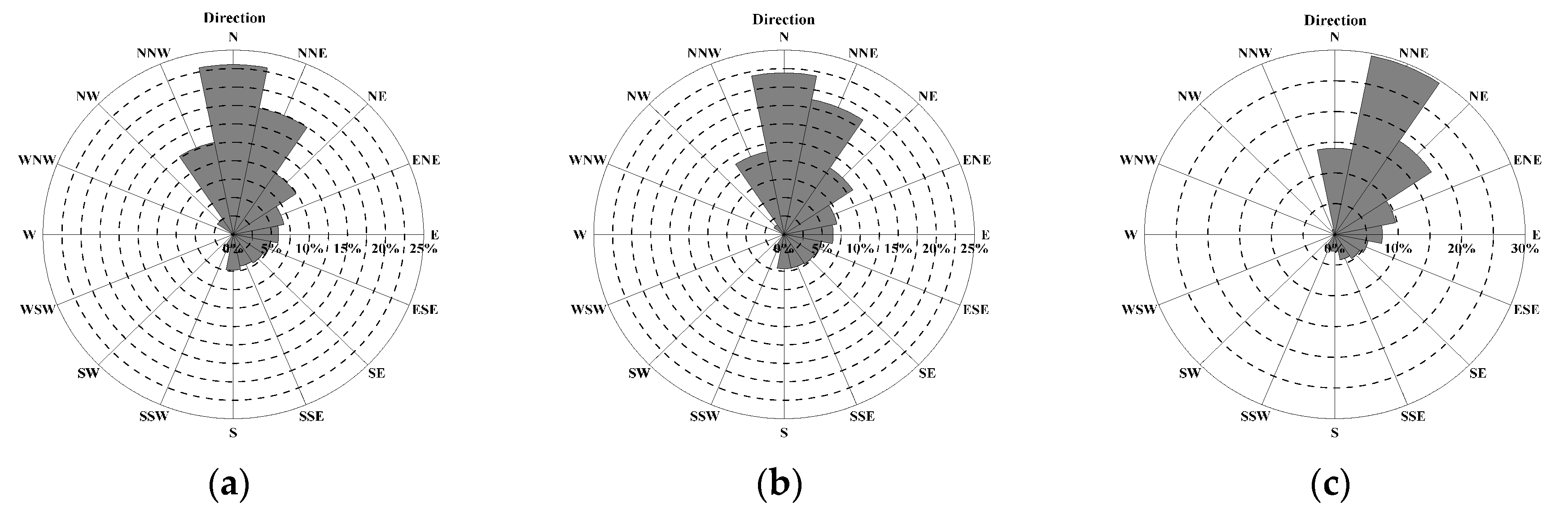
The directionality of the wave energy’s propagation is very meaningful to improve the conversion efficiency of WECs. Generally, the incident wave, which is orthometric with WECs, has the highest absorbance efficiency [27]. The directionality of the wave energy’s propagation is only of interest for certain WECs, such as oscillating wave surge converters (OWSCs), but not for axi-symmetric devices. In addition, the wave energy in extreme sea-states can never be exploited. Therefore, we must consider the influence of extreme sea-states when analyzing the directionality of exploitable wave energy. This study examined the directionality of the wave energy’s propagation under operational and extreme sea-states for key locations in the relatively nearshore waters of the Zhoushan Islands based on ERA-Interim data over the last 36 years for certain WECs. An operational sea-state is the sea-state with Hs < 4 m, indicating that the wave energy is exploitable, and an extreme sea-state is a sea-state with Hs ≥ 4 m, indicating that the wave energy is not exploitable. The percentage of the energy distribution in each direction was calculated separately for operational and extreme sea-states, and the wave power roses are plotted in Figure 10 and Figure 11. The direction of the dominant wave power for the operational sea-states at Location S1 was NNW-NE (clockwise direction), and the wave power accounted for approximately 63.08% of the total exploitable wave energy. At Location S2, the direction of the dominant wave power was NNW-NE, and the wave power accounted for approximately 62.83% of the total exploitable wave energy. At Location S3, the direction of the dominant wave power was N-ENE, and the wave power accounted for approximately 71.67% of the total exploitable wave energy. The directionality of the exploitable wave energy’s propagation was basically consistent in the key locations in the relatively nearshore waters of the Zhoushan Islands. The direction of the dominant wave power was mainly in the N and NNE directions because the influence of the northeastern monsoon is prominent in these areas; the waves are rough in the northeastern direction, and wave energy is relatively abundant. These results can serve as a reference to determine the operational direction of WECs. The direction of extreme waves for extreme sea-states at Location S1 was N-SE, and the wave power accounted for approximately 86.26% of the total extreme wave energy. At Location S2, the direction of extreme wave was N-SE, and the wave power accounted for approximately 87.68% of the total extreme wave energy. At Location S3, the direction of extreme wave was NNE-SSE, and the wave power accounted for approximately 91.80% of the total extreme wave energy. These results show that extreme waves mainly originated from the N-SSE directions because of cold swells from northeastern monsoons during winter and storms from the western Pacific during summer. This finding is of interest to developers.
5.3. Distribution of the Wave Energy Density According to the Wave Condition
When designing WECs, we must consider the range of wave conditions to improve the conversion efficiency. These conditions are the dominant contribution to the total wave energy density (the mean of the sum of Pw multiplied by the number of hours in a year MWh/(m·year)) and can be an important index for the design of WECs [24]. Based on the ERA-Interim data over the last 36 years by using an Hs interval of 0.5 m and a Te interval of 1 s, we calculated the percentage of the total wave energy density under each wave condition to the total wave energy density under all wave conditions; the results are shown in Figure 12. In this figure, the color code denotes the percentage and the number denotes the annual average number of times for each wave condition. At Locations S1, S2 and S3, the dominant wave conditions all had Hs values of 0.5–4.0 m and Te values of 4–9 s (the dominant wave condition is the range of wave conditions in which the wave energy accounts for 85% of the total wave energy density). Within this wave state, the wave energy accounted for 92.58%, 90.73% and 85.96% of the total wave energy density, respectively. The dominant wave conditions in the key relatively nearshore locations were the same and thus can act as a uniform standard for the design of WECs. WECs that are designed according to this standard can achieve higher conversion efficiency. In addition, the number of occurrences of wave condition with an Hs value of 0.5–1.0 m and a Te value of 5–6 s at Locations S1 and S2 was the highest, occurring 289 and 274 times and accounting for 4.95% and 4.50% of the total wave energy density, respectively. At Location S3, the number of occurrences of the wave condition with an Hs value of 1.0–1.5 m and a Te value of 5–6 s was the highest, occurring 211 times and accounting for 6.63% of the total wave energy density. However, the ratio of the wave energy under the most common wave conditions to the total wave energy density was not the highest. At Locations S1, S2 and S3, the wave condition with the highest ratio of the total wave energy density was that with an Hs value of 2.0–2.5 m and a Te value of 6–7 s. At each location, the annual average occurrences of the wave condition with the highest ratio of the total wave energy density were 70, 74 and 88, accounting for 11.84%, 11.67% and 11.37% of the total wave energy density, respectively. These results show that the contribution of the wave conditions to the most frequent ratio was not the most important factor.
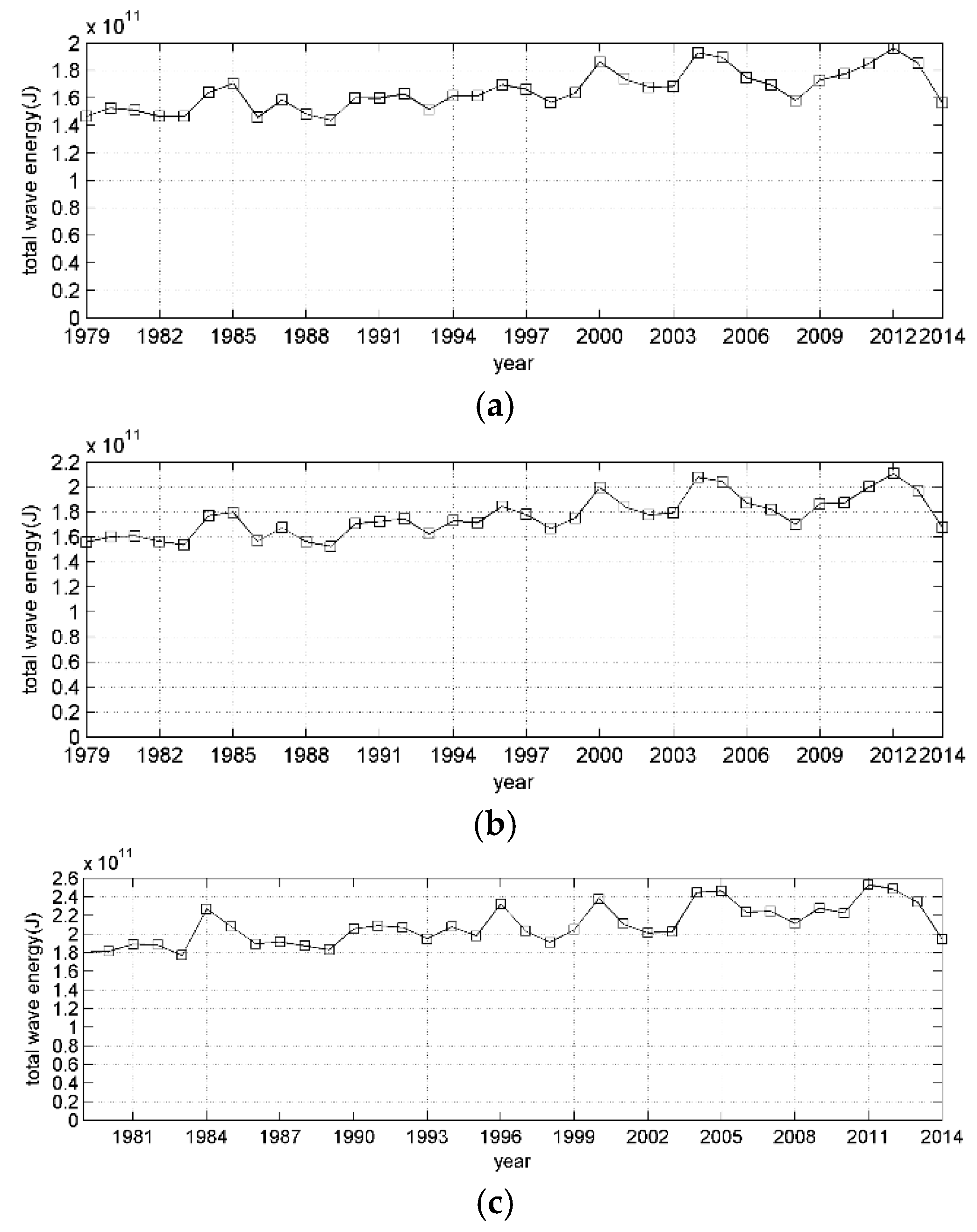
5.4. Inter-Annual Variation in the Total Wave Energy
The inter-annual variation in the total wave energy can effectively express the duration and stability of the wave energy over the long term at each location. This index is important to reasonably position WECs. Based on ERA-Interim data over the last 36 years, the total wave energy in the range of 0.125 × 0.125 was calculated for each year in the relatively nearshore key locations. The inter-annual variation in the total wave energy for each location is shown in Figure 13. This figure shows that the total wave energy of Locations S1, S2 and S3 in each year is higher than 1.4 × 10¹¹, 1.5 × 10¹¹, and 1.7 × 10¹¹, respectively. The wave energy in each location and year was sustainable, and the variation in the wave energy was small, which is advantageous to the development of wave energy projects.
5.5. Survivability and Use Ratio for Wave Energy Development
We must consider the survivability and practical use ratio for wave energy development in addition to the abundance level, the direction distributions, the wave energy distributions according to the wave condition, and the total wave energy.
The survivability refers to the allowable maximum sea state in which a WEC can operate normally. The maximum sea state must be defined by WEC developers so that they can design their machines to withstand, but this has a cost. When the sea state is higher, the cost of designing a WEC for survivability is also higher. The maximum sea state can be expressed by the maximum wave power density (Pmax, kW/m). When Pmax is higher, the cost of designing a WEC for survivability is also higher. Based on ERA-Interim data over the last 36 years, Pmax was calculated in the relatively nearshore key locations. The results are shown in Table 6. At each location, Pmax showed small differences, and the maximum Pmax was 385.30 kW/m, which can be used as a standard for developers to design WECs for survivability. The results in this paper can be a reference for the design of WECs in the relatively nearshore key locations of the Zhoushan Islands.
The practical use ratio is the percentage of the energy of the dominant wave condition that can be effectively converted by the WECs designed according to the standard in Section 5.3. The practical use ratio for the wave energy can be expressed as the ratio of the wave energy in the dominant wave condition to the total wave energy, where the dominant wave condition is defined as in Section 5.3. Based on the ERA-Interim data over the last 36 years, this value was calculated for each location, and the results are shown in Section 5.3. The results show that at each location, the practical use ratios were all greater than 85%. Thus, the practical use ratio for wave energy is high, and the development value of the wave energy is high in the key relatively nearshore locations of the Zhoushan Islands.
5.6. Performance Assessment of Wave Energy Converters
Compared to theoretical wave energy, decision makers that evaluate wave energy projects care more about the conditions of exploitable wave energy, which is more valuable for wave energy development. In this field, Folley and Whittaker [36] indicated that the exploitable wave energy resources in relatively nearshore waters can be defined by the average wave power that propagates in a fixed direction and is limited to a multiple of four times the average wave power. This work can provide reference for exploitable wave energy assessment. In Section 5.2, Section 5.3, Section 5.4 and Section 5.5, we evaluated some characteristics of the theoretical wave energy, which may be useful for the design, placement and operation of WECs in key locations. However Rusu and Soares [37] indicated that the actual wave power yield depends on the particular WEC device as rated by its wave power generation because each technology has different operational ranges and different efficiencies under various sea states. We must estimate the energy production of some proposed state of the art WECs to develop a pilot plant of wave energy in these key locations, which may be more useful for the practical development of wave energy. In this paper, we refer to the work of Vannucchi and Cappietti [38], who evaluated the performances of six different state of the art WECs to find which device was the best suited for Italian areas. This work is meaningful for wave energy development.
In this paper, we selected five different state of the art WECs that were used by Vannucchi and Cappietti [38], including AquaBuoy (>50 m) [39], AWS (>50 m) [40], Pelamis (>50 m) [41], Oyster (≈15 m) [42] and Wave Star (Nearshore) [43], by considering the water depths of S1, S2 and S3 (62 m, 60 m, 16 m, respectively) and the suitable water depths of these WECs. The main features of these WECs are shown in Vannucchi and Cappietti [38]. Then, we employed three indices, including the electricity production (Pe, kW), capacity factor (Cf, %) and capture width (Cw, m), which were indicated by Vannucchi and Cappietti [38] to analyze the energy production and determine the best suited WEC in each key location off the coast of China around the Zhoushan Islands. The formulas of these three indices are shown in Equations (13)–(15) [38]:
where nT is the number of Te classes and nH is the number of Hs classes. Pij is the power output of the device, which originates from the power matrix for the specific WEC. The power matrices of the WECs that were selected in this paper were collected from the open literature [32,44,45]. fij is the occurrence frequency for various sea states, which was collected from scatter diagrams [37]. The rated power (unit: kW) is the rated power of the WEC. The rated power of the WECs in this paper were 250 kW (AcquaBuoy); 2000 kW (AWS); 750 kW (Pelamis); 800 kW (Oyster) and 600 kW (Wave Star). Pw (unit: kW/m) is the annual average flux of energy in each key location. It is very important to note that because different devices have vastly different size, the capture width is not a good measure for comparison. So we employed the relative capture width (Rcw, %) instead of the capture width to compare the performance of WECs. The relative capture width is defined as Equation (16):
where main_dimension is a main dimension of WECs. A main dimension of AcquaBuoy is about 20 m [39]; AWS is 144 m [46]; Pelamis is 180 m [47]; Oyster is 26 m [42]; WS is 70 m [32].
Based on the above methodology and the ERA-Interim reanalysis wave field data from 1979 to 2014, we calculated the mean power output, capacity factor and relative capture width in each key location. The results are shown in Table 7. The highest capacity value was obtained for Pelamis in Location S1, where the capacity factor was 5.09%, the mean power output was 38.16 kW, but the relative capture width was 3.24%. The best relative capture width in Location S1 was obtained for AB with 8.05%. The results in Location S2 were similar to those in Location S1. Locations S1 and S2 were located in the relatively nearshore waters to the east of the Zhoushan Islands, where the water depth are approximately 60 m, so Pelamis looks like the best suited WEC when considering capacity factor and AB looks like the best suited WEC when considering relative capture width for this area. For Location S3, which is located in the nearshore waters to the southeast of the city of Taizhou and where the water depth is approximately 16 m, Wave Star looks like the best suited WEC when considering capacity factor, with a capacity factor of 18.38%, mean power output of 110.31 kW; Oyster looks like the best suited WEC when considering relative capture width, with relative capture width of 21.58%. But unfortunately, the rather poor capacity factors reported in Table 7 for the different WECs support the non-suitability of this wave climate for present state of the art WECs. In order to achieve cost efficient wave energy conversion, we must develop more suitable WECs for this areas. In addition, the wave farms are mainly constructed in nearshore shallow waters because of the limitation of technology and the cost of energy transmission. When comparing the performances of the state of the art WECs in Locations S1, S2 and S3, the mean power output was higher in Location S3 than in S1 and S2, and the capacity factor and relative capture width were higher too for all WECs.
5.7. Discussion for Wave Energy in Key Locations in the Relatively Nearshore Waters
The key locations in the relatively nearshore waters were in areas A5, A6 and A9, which included the relatively nearshore waters to the east of the Zhoushan Islands and to the relatively nearshore waters southeast of the city of Taizhou, Zhejiang Province. The direction of the dominant wave power under operational sea states was mainly in the N and NNE directions, which can serve as a reference to determine the operational direction of certain WECs when acquiring wave energy. Extreme waves mainly originated from the N-SSE directions because of cold swells and storms, which is of interest to developers. The dominant wave conditions all had an Hs value of 0.5–4.0 m and a Te value of 4–9 s, and the wave energy accounted for 85% of the total wave energy density; which can be a uniform standard for the design of new WECs that are suitable for these local areas. The wave energy in these key locations was sustainable for each year, and the variation in the wave energy was small, which is advantageous for the development of wave energy projects. The maximum wave power density was 385.30 kW/m, which can be used as a standard for developers to design WECs for survivability. Additionally, the practical use ratios for the wave energy were all greater than 85%. Furthermore, at present, there is no suitable state of the art WECs for cost efficient wave energy conversion in 3 key locations in the relatively nearshore waters of the Zhoushan Islands.
6. Conclusions
Based on high-resolution and high-accuracy ERA-Interim reanalysis wave field data from 1979 to 2014, the temporal and spatial distributions and the development potential of wave energy were studied in detail in offshore and relatively nearshore (key region) waters of the sea areas adjacent to the Zhoushan Islands. The conclusions are as follows:
- (1)
- The most suitable wave energy development areas in the offshore waters of the Zhoushan Islands are the eastern relatively nearshore sea areas of the Zhoushan Islands. Wave farms are more difficult to construct in offshore deep water areas and the cost of energy transmission is higher. Therefore, the east relatively nearshore sea areas of the Zhoushan Islands are a better choice for wave energy development. Although wave energy is not abundant in this area compared to global wave energy resources. Nonetheless, the wave energy here is still usable and stable and can serve as a suitable ocean renewable energy for the energy supply of the Zhoushan Islands.
- (2)
- The direction of the dominant wave power under operational and extreme sea states obtained in this paper is interesting to the operation of WECs and the developers of wave energy. The dominant wave conditions were all for a significant wave height of 0.5–4.0 m and an energy period of 4–9 s, and the maximum wave power density could reach 385.30 kW/m. These results can provide references for the design of new suitable WECs. Among existing WECs, there is no suitable state of the art WECs for cost efficient wave energy conversion in 3 key locations. The best location for wave energy development is located in the relatively nearshore waters to the southeast of the city of Taizhou (Location S3).
Acknowledgments
The authors would like to acknowledge the ECMWF for providing the ERA-Interim datasets and acknowledge support of the Natural Science Foundation of Shandong Province, China (Grant No. ZR2016DL09), “the Fundamental Research Funds for the Central Universities”, China (Grant No. 16CX02033A), the Fund of Oceanic Telemetry Engineering and Technology Research Center, State Oceanic Administration, China (Grant No. 2016005), the Dragon III Project from the Ministry of Science and Technology of China and the European Space Agency (Grant No. 10412) and the Ocean Renewable Energy Special Fund Project of the State Oceanic Administration of China (Grant No. GHME2011ZC07). The authors would like to express special thanks to the editors and anonymous reviewers for their constructive comments on this manuscript.
Author Contributions
All authors contributed to the research in the paper. Yong Wan searched the literature, designed the study, analyzed the data and wrote the paper; Chenqing Fan designed the study and analyzed the data; Jie Zhang and Junmin Meng designed the study; Yongshou Dai designed the study and analyzed the data; Ligang Li and Weifeng Sun analyzed the data and painted the figures; Peng Zhou performed the data interpretation; Jing Wang performed the data interpretation and designed the study; Xudong Zhang searched the literature and wrote the paper.
Conflicts of Interest
The authors declare no conflict of interest.
References
- Cornett, A.M. (Ed.) A global wave energy resource assessment. In Proceedings of the 18th International Conference on Offshore and Polar Engineering, Vancouver, BC, Canada, 6–11 July 2008. [Google Scholar]
- Barstow, S.; Mork, G.; Lonseth, L.; Petter, M.J. (Eds.) WorldWaves wave energy resource assessments from the deep ocean to the coast. In Proceedings of the 8th European Wave and Tidal Energy Conference; Uppsala Universitet: Uppsala, Sweden, 2009. [Google Scholar]
- Mork, G.; Barstow, S.; Kabuth, A.; Pontes, M.T. (Eds.) Assessing the global wave energy potential. In Proceedings of the ASME 2010 29th International Conference on Ocean, Offshore and Arctic Engineering, Shanghai, China, 6–11 June 2010. [Google Scholar]
- Arinaga, R.A.; Cheung, K.F. Atlas of global wave energy from 10 years of reanalysis and hindcast data. Renew. Energy 2012, 39, 49–64. [Google Scholar] [CrossRef]
- Zheng, C.W.; Shao, L.T.; Shi, W.L.; Su, Q.; Lin, G.; Li, X.Q. An assessment of global ocean wave energy resources over the last 45 a. Acta Oceanol. Sin. 2014, 33, 92–101. [Google Scholar] [CrossRef]
- Pontes, M.T.; Athanassoulis, G.A.; Brastow, S.; Cavaleri, L.; Holmes, B.; Mollison, D.; Oliveira-Pires, H. An atlas of wave energy resource in Europe. J. Offshore Mech. Arct. Eng. 1996, 118, 307–309. [Google Scholar] [CrossRef]
- Pontes, M.T. Assessing the European wave energy resource. J. Offshore Mech. Arct. Eng. 1998, 120, 226–231. [Google Scholar] [CrossRef]
- Soares, C.G.; Bento, A.R.; Goncalves, M.; Silva, D.; Martinho, P. Numerical evaluation of the wave energy resources along the Atlantic European coast. Comput. Geosci. 2014, 71, 37–49. [Google Scholar] [CrossRef]
- Henfridsson, U.; Neimane, V.; Strand, K.; Kapper, R.; Bernhoff, H.; Danielsson, O.; Leijon, M.; Sundberg, J.; Thorburn, K.; Ericsson, E.; et al. Wave energy potential in the Baltic Sea and the Danish part of the North Sea, with reflections on the Skagerrak. Renew. Energy 2007, 32, 2069–2084. [Google Scholar] [CrossRef]
- Zheng, C.W.; Zhuang, H.; Li, X.; Li, X.Q. Wind energy and wave energy resources assessment in the East China Sea and South China Sea. Sci. China Technol. Sci. 2012, 55, 163–173. [Google Scholar] [CrossRef]
- Zheng, C.W.; Pan, J.; Li, J.X. Assessing the China Sea wind energy and wave energy resources from 1988 to 2009. Ocean Eng. 2013, 65, 39–48. [Google Scholar] [CrossRef]
- Zheng, C.W.; Li, C.Y. Variation of the wave energy and significant wave height in the China Sea and adjacent waters. Renew. Sustain. Energy Rev. 2015, 43, 381–387. [Google Scholar] [CrossRef]
- Zheng, C.W.; Li, C.Y.; Pan, J.; Liu, M.Y.; Xia, L.L. An overview of global ocean wind energy resources evaluation. Renew. Sustain. Energy Rev. 2016, 53, 1240–1251. [Google Scholar] [CrossRef]
- Kim, G.; Jeoug, W.M.; Lee, K.S.; Jun, K.; Lee, M.E. Offshore and nearshore wave energy assessment around the Korean Peninsula. Energy 2011, 36, 1460–1469. [Google Scholar] [CrossRef]
- Iglesias, G.; Carballo, R. Wave energy potential along the Death Coast (Spain). Energy 2009, 34, 1963–1975. [Google Scholar] [CrossRef]
- Iglesias, G.; Lopez, M.; Carballo, R.; Castro, A.; Fraguela, J.A.; Frigaard, P. Wave energy potential in Galicia (NW Spain). Renew. Energy 2009, 34, 2323–2333. [Google Scholar] [CrossRef]
- Iglesias, G.; Carballo, R. Offshore and inshore wave energy assessment: Asturias (N Spain). Energy 2010, 35, 1964–1972. [Google Scholar] [CrossRef]
- Iglesias, G.; Carballo, R. Wave energy resource in the Estaca de Bares area (Spain). Renew. Energy 2010, 35, 1574–1584. [Google Scholar] [CrossRef]
- Iglesias, G.; Carballo, R. Wave power for La Isla Bonita. Energy 2011, 35, 5013–5021. [Google Scholar] [CrossRef]
- Iglesias, G.; Carballo, R. Choosing the site for the first wave farm in a region: A case study in the Galician Southwest (Spain). Energy 2011, 36, 5525–5531. [Google Scholar] [CrossRef]
- Liang, B.C.; Fan, F.; Liu, F.S.; Gao, S.H.; Zuo, H.Y. 22-Year wave energy hindcast for the China East Adjacent Seas. Renew. Energy 2014, 71, 200–207. [Google Scholar] [CrossRef]
- Zheng, C.W.; Lin, G.; Shao, L.T. Wave energy resources analysis around Taiwan waters. J. Nat. Resour. 2013, 28, 1179–1186. [Google Scholar]
- Li, R.L. Research on Various Periods of Sea Waves. Master’s Thesis, Ocean University of China, Qingdao, China, 2007. [Google Scholar]
- Wan, Y.; Zhang, J.; Meng, J.M.; Wang, J. Wave energy assessment in the East China Sea and South China Sea based on ERA-Interim high resolution data. Acta Energiae Sol. Sin. 2015, 36, 1259–1267. [Google Scholar]
- Zheng, C.W.; Jia, B.K.; Guo, S.P.; Zhuang, H. Wave energy resource storage assessment in global ocean. Resour. Sci. 2013, 35, 1611–1616. [Google Scholar]
- Stopa, J.E.; Cheung, K.F.; Chen, Y.L. Assessment of wave energy resources in Hawaii. Renew. Energy 2011, 36, 554–567. [Google Scholar] [CrossRef]
- Wang, C.K.; Lu, W. Analysis Methods and Reserves Evaluation of Ocean Energy Resources; Ocean Press: Beijing, China, 2009; pp. 104–129. [Google Scholar]
- Smith, W.H.F.; Sandwell, D.T. Global seafloor topography from satellite altimetry and ship depth soundings. Science 1997, 277, 1957–1962. [Google Scholar] [CrossRef]
- Wen, S.C.; Yu, Z.W. Ocean Wave Theory and Calculation Principle; Science Press: Beijing, China, 1985; pp. 203–204. [Google Scholar]
- Wan, Y.; Zhang, J.; Meng, J.M.; Wang, J. Exploitable wave energy assessment based on ERA-Interim reanalysis data—A case study in the East China Sea and the South China Sea. Acta Oceanol. Sin. 2015, 34, 143–155. [Google Scholar] [CrossRef]
- Cruz, J. Ocean Wave Energy Current Status and Future Prespectives; Springer: Berlin/Heidelberg, Germany, 2008; p. 95. [Google Scholar]
- Marquis, L.; Kramer, M.; Frigaard, P. (Eds.) First power production results from the Wave Star Roshage wave energy converter. In Proceedings of the 3rd International Conference on Ocean Energy, Bilbao, Spain, 6–8 October 2010; Available online: http://wavestarenergy.com/sites/default/files/Wave%20Star%20Energy%20presentation%20ICOE%202010%20UPDATED%20After%20Conference.pdf (accessed on 9 January 2016).
- Ma, H.S.; Yu, Q.W. The preliminary estimate for the potential surface wave energy resources in the adjacent sea areas of China. Mar. Sci. Bull. 1983, 2, 73–81. [Google Scholar]
- Li, L.P.; Tian, S.Z.; Xu, S.L.; Guo, H.M. Power resource estimation of ocean surface waves in the Bohai Sea and Yellow Sea and an evaluation of prospects for converting wave power. J. Oceanogr. Huanghai Bohai Seas 1984, 2, 14–23. [Google Scholar]
- Ren, J.L.; Luo, Y.Y.; Zhong, Y.J.; Xu, Z. The implementation for analysis system of ocean wave resources and the application of wave energy power generation. J. Zhejiang Univ. Technol. 2008, 36, 186–191. [Google Scholar]
- Folley, M.; Whittaker, T.J.T. Analysis of the nearshore wave energy resource. Renew. Energy 2009, 34, 1709–1715. [Google Scholar] [CrossRef]
- Rusu, L.; Soares, C.G. Wave energy assessments in the Azores islands. Renew. Energy 2012, 45, 183–196. [Google Scholar] [CrossRef]
- Vannucchi, V.; Cappietti, L. Wave energy assessment and performance estimation of state of the art wave energy converters in Italian hotspots. Sustainability 2016, 8, 1300. [Google Scholar] [CrossRef]
- Weinstein, A.; Fredrikson, G.; Parks, M.J.; Nielsen, K. (Eds.) AquaBuOY—The offshore wave energy converter numerical modeling and optimization. In Proceedings of the OCEANS’04, Kobe, Japan, 9–12 November 2004. [Google Scholar]
- Valério, D.; Beirão, P.; Sá da Costa, J. Optimisation of wave energy extraction with the Archimedes Wave Swing. Ocean Eng. 2007, 34, 2330–2344. [Google Scholar] [CrossRef]
- Henderson, R. Design, simulation, and testing of a novel hydraulic power take-off system for the Pelamis wave energy converter. Renew. Energy 2006, 31, 271–283. [Google Scholar] [CrossRef]
- Whittaker, T.J.T.; Collier, D.; Folley, M.; Osterreid, M.; Henry, A.; Crowley, M. (Eds.) The development of Oyster—A shallow water surging wave energy converter. In Proceedings of the 7th European Wave & Tidal Energy Conference, Porto, Portugal, 11–13 September 2007; Available online: https://www.researchgate.net/publication/228671649_The_development_of_Oyster-A_shallow_water_surging_wave_energy_converter (accessed on 9 January 2016).
- Kramer, M.; Marquis, L.; Frigaard, P. (Eds.) Performance evaluation of the wavestar prototype. In Proceedings of the 9th European Wave and Tidal Energy Conference, Southampton, UK, 5–9 September 2011; Available online: http://www.energinet.dk/SiteCollectionDocuments/Danske%20dokumenter/Forskning%20-%20PSOprojekter/Bilag%203%20-%20Performance%20Evaluation%20of%20the%20Wavestar%20Prototype%20-%20M.%20M.%20Kramer%20et%20al.pdf (accessed on 9 January 2016).
- Silva, D.; Rusu, E.; Soares, C.G. Evaluation of various technologies for wave energy conversion in the Portuguese Nearshore. Energies 2013, 6, 1344–1364. [Google Scholar] [CrossRef]
- Carbon, T. Variability of UK Marine Resources; Environmental Change Institute: Oxford, UK, 2005. Available online: https://tethys.pnnl.gov/sites/default/files/publications/Carbon_Trust_2005.pdf (accessed on 9 January 2016).
- AWS-III Multi-Cell Wave Power Generator. AWS Ocean Energy Ltd, 2017. Available online: http://www.awsocean.com/ (accessed on 9 January 2016).
- Pelamis Is the Result of over a Decade of Dedicated Testing, Modelling and Development. Pelamis Wave Power Ltd, 2017. Available online: http://www.pelamiswave.com/homepage/search/ (accessed on 9 January 2016).
Figure 1.
Location of the area of interest.

Figure 2.
Locations of the buoys.

Figure 3.
Comparisons of the wave fields from ERA-Interim: (a) buoy 006’s significant wave height; (b) buoy 006’s energy period; (c) buoy kzszs’s significant wave height; and (d) buoy kzszs’s energy period.
Figure 3.
Comparisons of the wave fields from ERA-Interim: (a) buoy 006’s significant wave height; (b) buoy 006’s energy period; (c) buoy kzszs’s significant wave height; and (d) buoy kzszs’s energy period.


Figure 4.
Multi-year annual average of the significant wave height for the sea areas adjacent to the Zhoushan Islands: (a) annual average; (b) winter average; (c) spring average; (d) summer average; and (e) autumn average.
Figure 4.
Multi-year annual average of the significant wave height for the sea areas adjacent to the Zhoushan Islands: (a) annual average; (b) winter average; (c) spring average; (d) summer average; and (e) autumn average.


Figure 5.
Multi-year annual average of the energy period for the sea areas adjacent to the Zhoushan Islands: (a) annual average; (b) winter average; (c) spring average; (d) summer average; and (e) autumn average.
Figure 5.
Multi-year annual average of the energy period for the sea areas adjacent to the Zhoushan Islands: (a) annual average; (b) winter average; (c) spring average; (d) summer average; and (e) autumn average.


Figure 6.
Multi-year annual average of the wave power density for the sea areas adjacent to the Zhoushan Islands: (a) annual average; (b) winter average; (c) spring average; (d) summer average; and (e) autumn average.
Figure 6.
Multi-year annual average of the wave power density for the sea areas adjacent to the Zhoushan Islands: (a) annual average; (b) winter average; (c) spring average; (d) summer average; and (e) autumn average.


Figure 7.
Distribution of the stability index for the sea areas adjacent to the Zhoushan Islands.

Figure 8.
Regional division results and the key locations.

Figure 9.
CDC contour plot for every grid in three key areas.

Figure 10.
Wave power rose for each key location under operational sea-states: (a) S1; (b) S2 and (c) S3.
Figure 10.
Wave power rose for each key location under operational sea-states: (a) S1; (b) S2 and (c) S3.

Figure 11.
Wave power rose for each key location under extreme sea-states: (a) S1; (b) S2 and (c) S3.
Figure 11.
Wave power rose for each key location under extreme sea-states: (a) S1; (b) S2 and (c) S3.

Figure 12.
The distributions of the total wave energy density according to the wave condition for each key location: (a) S1; (b) S2; and (c) S3.
Figure 12.
The distributions of the total wave energy density according to the wave condition for each key location: (a) S1; (b) S2; and (c) S3.

Figure 13.
Distributions of the total wave energy’s inter-annual variation for each key location: (a) S1; (b) S2; and (c) S3.
Figure 13.
Distributions of the total wave energy’s inter-annual variation for each key location: (a) S1; (b) S2; and (c) S3.


Table 1.
Buoy specifications.
| Buoy ID | Location | Water Depth (m) | Data Period | Time Interval |
|---|---|---|---|---|
| buoy_006 | 30.7170 (°N), 123.0700 (°E) | 46 | April 2012–Decmber 2012 | 10 (min) |
| buoy_kzszs | 29.7527 (°N), 122.7500 (°E) | 42 | April 2012–Decmber 2012 | 10 (min) |
Table 2.
Error indices that were used to compare the ERA-Interim and buoys.
| Buoy | RMSE | CC |
|---|---|---|
| Buoy 006 Hs | 0.31 (m) | 0.90 |
| Buoy 006 Te | 0.56 (s) | 0.78 |
| Buoy kzszs Hs | 0.36 (m) | 0.78 |
| Buoy kzszs Te | 0.81 (s) | 0.70 |
Table 3.
Criterion of the regional division (general form).
| Grade | Annual Average Pw (kW/m) | Annual Average TE (h) | TWE (×1012 J) | CDC | Suitability Level |
|---|---|---|---|---|---|
| 1 | <a1 | <b1 | <c1 | <d1 | poor |
| 2 | a1–a2 | b1–b2 | c1–c2 | d1–d2 | available |
| 3 | a2–a3 | b2–b3 | c2–c3 | d2–d3 | good |
| 4 | a3–a4 | b3–b4 | c3–c4 | d3–d4 | better |
| 5 | >a4 | >b4 | >c4 | >d4 | best |
Table 4.
Thresholds for each index.
| Index | Maximum Value | Minimum Value | Interval | a1/b1/c1 | a2/b2/c2 | a3/b3/c3 | a4/b4/c4 |
|---|---|---|---|---|---|---|---|
| Annual average Pw (kW/m) | 5.57 | 2.04 | 0.71 | 2.75 | 3.46 | 4.17 | 4.88 |
| Annual average TE (h) | 4367 | 1812 | 511 | 2323 | 2834 | 3345 | 3856 |
| TWE (×1012 J) | 2.3053 | 0.9516 | 0.2707 | 1.2223 | 1.4930 | 1.7637 | 2.0344 |
Table 5.
Criterion of the regional division for the relatively nearshore waters of the Zhoushan Islands.
Table 5.
Criterion of the regional division for the relatively nearshore waters of the Zhoushan Islands.
| Grade | Pw (kW/m) | TE (h) | TWE (×1012 J) | CDC | Suitability Level |
|---|---|---|---|---|---|
| 1 | <2.75 | <2323 | <1.2223 | <7808 | poor |
| 2 | 2.75–3.46 | 2323–2834 | 1.2223–1.4930 | 7808–14,639 | available |
| 3 | 3.46–4.17 | 2834–3345 | 1.4930–1.7637 | 14,639–24,601 | good |
| 4 | 4.17–4.88 | 3345–3856 | 1.7637–2.0344 | 24,601–38,282 | better |
| 5 | >4.88 | >3856 | >2.0344 | >38,282 | best |
Table 6.
Wave energy indexes results in each key location.
| Location | Longitude (°E) | Latitude (°N) | Water Depth D (m) | Annual Average Pw (kW/m) | Pmax (kW/m) |
|---|---|---|---|---|---|
| S1 | 123.250 | 30.375 | 62 | 6.53 | 290.72 |
| S2 | 123.250 | 29.875 | 60 | 7.01 | 385.30 |
| S3 | 121.875 | 28.375 | 16 | 9.55 | 322.14 |
Table 7.
Mean power output, capacity factor and relative capture width in each key location.
| Location | Mean Power Output “Pe” (kW) | Capacity Factor “Cf” (%) | Relative Capture Width “Rcw” (%) | ||||||||||||
|---|---|---|---|---|---|---|---|---|---|---|---|---|---|---|---|
| AB AWS Pelamis Oyster WS | AB AWS Pelamis Oyster WS | AB AWS Pelamis Oyster WS | |||||||||||||
| S1 | 10.52 | 25.26 | 38.16 | - | - | 4.21 | 1.26 | 5.09 | - | - | 8.05 | 2.69 | 3.24 | - | - |
| S2 | 11.47 | 28.27 | 41.51 | - | - | 4.59 | 1.41 | 5.53 | - | - | 8.20 | 2.80 | 3.29 | - | - |
| S3 | - | - | - | 56.61 | 110.31 | - | - | - | 6.70 | 18.38 | - | - | - | 21.58 | 16.50 |
© 2017 by the authors. Licensee MDPI, Basel, Switzerland. This article is an open access article distributed under the terms and conditions of the Creative Commons Attribution (CC BY) license (http://creativecommons.org/licenses/by/4.0/).
Share and Cite
MDPI and ACS Style
Wan, Y.; Fan, C.; Zhang, J.; Meng, J.; Dai, Y.; Li, L.; Sun, W.; Zhou, P.; Wang, J.; Zhang, X. Wave Energy Resource Assessment off the Coast of China around the Zhoushan Islands. Energies 2017, 10, 1320. https://doi.org/10.3390/en10091320
AMA Style
Wan Y, Fan C, Zhang J, Meng J, Dai Y, Li L, Sun W, Zhou P, Wang J, Zhang X. Wave Energy Resource Assessment off the Coast of China around the Zhoushan Islands. Energies. 2017; 10(9):1320. https://doi.org/10.3390/en10091320
Chicago/Turabian StyleWan, Yong, Chenqing Fan, Jie Zhang, Junmin Meng, Yongshou Dai, Ligang Li, Weifeng Sun, Peng Zhou, Jing Wang, and Xudong Zhang. 2017. "Wave Energy Resource Assessment off the Coast of China around the Zhoushan Islands" Energies 10, no. 9: 1320. https://doi.org/10.3390/en10091320
Note that from the first issue of 2016, this journal uses article numbers instead of page numbers. See further details here.