Article

Energy Flexibility Management Based on Predictive Dispatch Model of Domestic Energy Management System

by
Amin Shokri Gazafroudi
1,*,
Francisco Prieto-Castrillo
1,2,3,
Tiago Pinto
1,
Javier Prieto
1,4,
Juan Manuel Corchado
1,5 and
Javier Bajo
1
1
BISITE Research Group, University of Salamanca, Edificio I+D+i, 37008 Salamanca, Spain
2
MediaLab, Massachusetts Institute of Technology, Cambridge, MA 02139-4307, USA
3
Harvard T.H. Chan School of Public Health, Harvard University, Boston, MA 02115, USA
4
StageMotion, R&D Department, C/Orfebres 10, 34005 Palencia, Spain
5
Osaka Institute of Technology, Asahi-ku Ohmiya, Osaka 535-8585, Japan
*
Author to whom correspondence should be addressed.
Energies 2017, 10(9), 1397; https://doi.org/10.3390/en10091397
Submission received: 3 August 2017 / Revised: 1 September 2017 / Accepted: 5 September 2017 / Published: 13 September 2017
(This article belongs to the Special Issue Distributed Energy Resources Management)

Abstract

:
This paper proposes a predictive dispatch model to manage energy flexibility in the domestic energy system. Electric Vehicles (EV), batteries and shiftable loads are devices that provide energy flexibility in the proposed system. The proposed energy management problem consists of two stages: day-ahead and real time. A hybrid method is defined for the first time in this paper to model the uncertainty of the PV power generation based on its power prediction. In the day-ahead stage, the uncertainty is modeled by interval bands. On the other hand, the uncertainty of PV power generation is modeled through a stochastic scenario-based method in the real-time stage. The performance of the proposed hybrid Interval-Stochastic (InterStoch) method is compared with the Modified Stochastic Predicted Band (MSPB) method. Moreover, the impacts of energy flexibility and the demand response program on the expected profit and transacted electrical energy of the system are assessed in the case study presented in this paper.

1. Introduction

1.1. Aims and Motivation

In the last decade, power systems have faced new challenges due to the increment of the distributed renewable energy resources. Renewable energy resources decrease the greenhouse gas emissions and costs related to electricity production [1]. However, the integration of these intermittent energy resources leads to energy management problems based on the scale of the energy system [2]. At a smaller scale, Domestic Energy Management Systems (DEMSs) enable the residential customers to manage their loads in order to minimize the electricity cost. Generally, there are two approaches for energy management of the DEMSs. These approaches consist of centralized and decentralized systems. Based on the approach of the system, different structures of the controlling and communicating systems are required [3].

1.2. Literature Review

Various research has been presented for optimal energy scheduling at the scale of the smart homes and smart grids that can be classified based on their goals, strategies, utilized technologies and software. In [4,5], the authors discussed the necessities of using computational intelligence in the DEMSs and a review of energy management systems based on multi-agent systems, respectively. On the other hand, in [6], the present and future perspectives regarding EVs and their operation modes in smart grids and smart homes have been discussed. In [7], the authors proposed a method to schedule the local energy resources optimally. Minimizing the loss of energy and purchasing electricity cost were the main goals of the authors. In [8], the authors defined the DEM problem in connection with local energy nodes. Furthermore, in [8], homes have a two-way communication with the market and can manage energy locally. In [9], a domestic demand response has been implemented in a distribution grid. The real-time price is the main goal of the demand response program based on the direct load control in [9]. Furthermore, the uncertainty of the price and load has been considered in [9]. Price prediction has been used instead of communication between homes in the distribution network.
In [10], a DEMS has been developed for day-ahead energy scheduling considering hourly pricing and the peak power constraint based on the demand response programs. The authors of [11] proposed a method to manage the energy of EV and energy storage systems according to the dynamic pricing, peak power limitation and demand response programs. The proposed Domestic Energy Management (DEM) problem has been modeled by mixed-integer linear programming. In [12], the authors propose a decentralize strategy for optimal energy scheduling under the large penetration of EVs. This interaction has been considered between consumers and the aggregator in [12]. This way, end-users send their optimum demand decisions and reschedule their demands based on the signals of the aggregator. In [13], a rescheduling DEMS has been presented to make the optimum decisions through the day and avoid the negative impact of price uncertainty.
The authors of [14] presented a multi-time scale DEM problem that includes EV and different types of electrical loads. Furthermore, the authors introduced the improved optimization algorithm to solve the DEM problem. In [15], a chance constraint model has been presented to optimize the performance of the domestic devices. The improved particle swarm optimization method has been used to optimize the problem based on the proposed demand response program. In [16], the authors introduced the Stackelberg game-based method to maximize the profits of the costumers and retailers simultaneously. In the proposed home model of [16], electrical loads of customers are elastic based on EVs. Furthermore, the price-based DR has been implemented in [16]. In [17], the DEM problem has been solved by stochastic dynamic programming considering EV. The authors proved that the EV is one source of uncertainty in the system due to the EV’s plug-in time, plug-out time and charge demand for mobility. Hence, the plug-state of the EV has been modeled through a Markov chain in [17]. In [18], a DEMS has been presented as part of an organization-based multi-agent system. Besides, the uncertainty of distributed energy resources has been considered through an Modified Stochastic Predicted Band (MSPB) method used to model the DEM problem.

1.3. Contributions

In the literature, several relevant advances have been accomplished in the DEMS domain. These mostly refer to the study and analysis of the several resources’ impact on the management process, namely flexible loads, EVs, batteries and generation. The interaction with the electricity market and the participation in demand response programs has also been explored, and this research is leading to promising outcomes, but modeling the electricity market at the local level has not been of interest to the authors in the previous works. However, the local electricity market has been introduced in [18], but the impact of the flexibility has not been evaluated in [18]. The research dealing with the uncertainty associated with the several resources is, however, still at an initial stage. Although some relevant works can be found in the literature, there are still many loose ends due to the difficulty in correctly identifying, measuring, modeling and representing the different sources of uncertainty, so that these can be correctly considered by DEMS scheduling, dispatch and management models.
In order to overcome the limitations in the field, this paper proposes a two-stage predictive dispatch model to manage energy flexibility in the domestic energy system. EV, battery and shiftable loads are in charge of providing the energy flexibility. A novel hybrid (InterStoch) method is defined for the first time in this paper to model the uncertainty of the PV power generation. In the first stage, the day-ahead stage, the uncertainty is modeled by interval bands. However, a stochastic scenario-based method is used to consider the uncertainty of PV power generation in the second stage, the real-time stage. Finally, the performance of the proposed hybrid Interval-Stochastic (InterStoch) method is compared with the MSPB method that was introduced in [18,19].
The rest of this paper is organized as follows. Section 2 introduces the proposed hybrid interval-stochastic method. Then, the domestic energy management problem is described in Section 3. Section 4 provides the simulation results. Finally, Section 5 summarizes the conclusions.

2. Interval-Stochastic Method

2.1. Data

In this paper, the predicted data from [18] have been used. For simplicity, only the uncertainty of PV power generation is considered. As shown in Table 1, the predicted data in each time step consist of the central forecasting and up/down deviation. Hence, the predicted data are limited to the upper/lower band based on the central forecasting and up/down deviation. It is noticeable that this paper concentrates only on modeling the uncertainty due to PV power prediction in the system. Hence, the forecasting system is not explained in this paper. The presented data of Table 1 are the inputs of the energy management system. Therefore, the energy management system makes optimum decisions through the InterStoch method.

2.2. Interval Model

In the day-ahead stage, PV system power generation is limited between bands according to the forecasting deviations. The minimum band represents the deviation below the central forecasting, and the maximum band represents the deviation above the central forecasting. P p v t d a intends to converge to the maximum/minimum band in the best/worst case. Therefore, Equation (1) can be divided into Equations (2) and (3) in the best and worst cases, respectively. This way, an auxiliary parameter is added in these equations as a slack parameter for the decision-maker. This parameter is denoted as the Optimistic Coefficient (OC), α , which is between zero and one, and had been defined for the first time in [19]. Hence, P p v t d a converges to the best/worst case when the decision-maker has the pessimistic/conservative perspective by adding α to Equations (2) and (3) and summing over them, as seen in Equation (4). Then, Equations (4) and (5) are obtained through simplification of Equations (1)–(3).
[ H ] P p v t p r e d σ p v t d o w n P p v t d a P p v t p r e d + σ p v t u p
P p v t p r e d P p v t d a P p v t d a + σ p v t u p : O C = 1
P p v t p r e d σ p v t d o w n P p v t d a P p v t p r e d : O C = 0
P p v t p r e d α p v ( P p v t p r e d σ p v t d o w n ) ( 1 α p v ) P p v t d a ( P p v t p r e d + σ p v t u p ) α p v + P p v t p r e d ( 1 α p v )
P p v t p r e d σ p v t d o w n ( 1 α p v ) P p v t d a P p v t p r e d + σ p v t u p α p v

2.3. Stochastic Model

In the real-time stage, stochastic programming is used to model the uncertainty of the PV power. Therefore, scenarios with their corresponding probabilities are defined in this section. This way, the prediction mean and deviation are defined as metric parameters by Equations (6) and (7), respectively. These are used to generate the scenarios of the PV power in the real-time stage. In this step, three scenarios are defined to model the uncertainty of the PV system’s power generation. The first scenario, the up scenario, describes data that have a deviation above the central forecasting. The second scenario, the down scenario, represents data that have a deviation below the central forecasting. Then, the third scenario describes the central forecasting data. The amounts of these scenarios are determined through Equations (8)–(10). Moreover, the corresponding probabilities are obtained according to Equations (11)–(13).
(6) P p v t m e a n = P p v t p r e d + σ p v t u p σ p v t d o w n 2 (7) Δ p v t = σ p v t u p + σ p v t d o w n 2 (8) P p v t r t ( ω = ω 1 ) = P p v t p r e d + σ p v t u p (9) P p v t r t ( ω = ω 2 ) = P p v t p r e d σ p v t d o w n (10) P p v t r t ( ω = ω 3 ) = P p v t p r e d (11) π ( ω = ω 1 ) = P r o b ( P p v t p r e d + σ p v t u p > P p v t m e a n + Δ p v t ) (12) π ( ω = ω 2 ) = P r o b ( P p v t p r e d σ p v t d o w n < P p v t m e a n Δ p v t ) (13) π ( ω = ω 3 ) = 1 π ( ω = ω 1 ) π ( ω = ω 2 )

3. Domestic Energy Management Problem

We consider that each smart home can participate in two different types of Local Electricity Market (LEM), not the wholesale market [18]. These LEMs are called day-ahead and real-time markets. In practice, the proposed LEMs can be operated by distribution system operator or retailers. Hence, the distribution system operator or retailers are responsible for providing the local electricity market framework for their agents that are in their region or have contracts to transact energy with them. Besides, it is considered that smart homes are price-takers in the LEM, and they can buy electricity from the local electricity market based on the Time of Use (ToU) tariff. Furthermore, it is assumed that the sold/bought electricity prices to/from the local electricity market are different. The domestic energy management problem is modeled as a two-stage problem. The first stage is called the day-ahead stage, and the second stage is called the real-time stage. Here, the Expected Profit (EP) is defined by an Objective Function (OF) to maximize the profit of energy services. In Equation (14), E P is the sum of the day-ahead EP, E P d a , and the real-time EP, E P r t , which are OFs of the day-ahead and real-time stages, respectively.
E P = E P d a + E P r t

3.1. Day-Ahead Stage

The objective function of the domestic energy management system in the day-ahead local electricity market is defined in the Day-Ahead (DA) stage. The purpose is to make the best decisions in each of the time periods during the day d. However, the DA stage obtains optimum decisions for the system in day d-1. Hence, the objective function for the DA stage is represented in (15):
E P d a = t = 1 N t ( λ t P p v , o u t t d a + k γ k λ t P d i s , o u t t d a ( k ) λ t P n e t t d a )
E P d a consists of three parts. The first and second parts represent the revenue of selling the electrical energy produced by PV and Energy Storage Systems (ESSs) to the local market. The third part states the costs of buying the electrical energy from the local market. It should be mentioned that participation factor, γ k , is a binary parameter that is defined for the first time in this paper in order to consider the participation of the ESSs in the DA stage. If the participation factor is equal to zero, ESSs are used to trade energy only in the real-time LEM. In other words, homes can utilize the full capacity of the ESSs in the day-ahead market if the participation factor equals one. The constraints of the DA stage are:
P n e t t d a + P p v , i n t d a + k γ k P d i s , i n t d a ( k ) = j = 1 N j L j t d a + γ k P c h t d a ( k )
S m a x P n e t t d a P p v , o u t t d a k γ k P d i s , o u t t d a ( k ) S m a x
Equation (16) establishes the power balance equation due to the power outputs of the PV, P p v , i n t d a , and ESSs, P d i s , i n t d a ( k ) , injected into the home, the grid power input, P n e t t d a , electrical loads, L j t d a , and the charged power of ESSs, P c h t d a ( k ) . In this paper, power loss is not considered for simplicity. Equation (17) represents the power flow limitation through the distribution line, which ends at the building. S m a x expresses the maximum power capacity of the distribution line that links the smart home with the distribution power network. Besides, there are some limitations corresponding to all appliances. Only the maximum and minimum limitations of the energy produced/consumed are defined in each device at this stage because the uncertainty is not considered in the DA stage.
(18) P p v t d a = P p v , i n t d a + P p v , o u t t d a (19) P p v t p r e d σ p v t d o w n ( 1 α p v ) P p v t d a P p v t p r e d + σ p v t u p α p v (20) L j t d a = L j t p r e d (21) j = 1 N j L j t d a = L s h t d a + L s w h t d a + L p p t d a + L m r s t d a
The total power generation of the PV is stated in (18). Equation (19) represents the power output limitations of the PV system. Besides, Equation (20) represents the total electrical power consumed.

Energy Storage Systems

ESSs can be utilized economically based on the charge and discharge strategies in the DEM problem. Mobility patterns and storage characteristics of the ESSs are different factors that should be considered in modeling the ESSs. However, the mobility pattern is only related to the EVs.
(22) C t d a ( k ) = C t 1 d a ( k ) + P c h t d a ( k ) η B 2 V P d i s t d a ( ω ) / η V 2 B ,   t 2 C t d a ( ω ) = C i ,   t = 1 (23) P e v m i n C t d a ( k ) P e v m a x (24) w m i n C t d a ( k ) C t 1 d a ( k ) w m a x ,   t 2 w m i n C t d a ( k ) C i ( k ) w m a x ,   t = 1 (25) 0 P d i s t d a ( k ) w m a x u t d a (26) 0 P c h t d a ( k ) w m i n ( 1 u t d a ) (27) P d i s t d a ( k ) = P d i s , i n t d a ( k ) + P d i s , o u t t d a ( k )

3.2. Real-Time Stage

In this stage, the objective function of the home due to participating in the RTLEM is defined. In addition, the uncertainties of decision-making variables are considered through a stochastic scenario-based method. These variables are determined based on the outputs of the first stage and the prediction engine. It is noticeable that the traded energy of the homes in the real-time market is different from their traded energy in the day-ahead market because of the PV power generation uncertainty. In other words, the traded energy of smart homes in real time can be positive or negative due to the prediction error of the PV power generation. The expected profit of the real-time stage, E P r t , is represented as:
E P r t = t = 1 N t ω = 1 N Ω π ( ω ) ( λ t ( P p v , o u t t r t ( ω ) P p v , o u t t d a ) + k ( λ t ( P d i s , o u t t r t ( k , ω ) γ k P d i s , o u t t d a ( k ) ) λ t ( P c h t r t ( ω ) γ k P c h t d a ( k ) ) ) j = 1 N j V O L L j L j t s h e d ( ω ) V p v s S p v t ( ω ) )
E P r t consisting of five parts. The first part represents the revenue for selling energy produced by PV to the real-time local electricity market. The total cost of electrical energy that is bought from the BLEMis represented in the second part. The third part expresses the profit due to selling the stored electrical energy of ESSs to the local market. The Value of Loss Load (VOLL) cost, V O L L j , is stated in the fourth part. Finally, the spillage cost of the PV system is represented in the last part. As seen in (28), it is proposed that if the PV power generation in the real-time stage, P p v , o u t t r t ( ω ) , is more than the PV power generation in the DA stage, the DEMS can only sell its extra power at the net price, λ , that is less than the price that is established for the purchase of the power generated by the PV on the day-ahead local market, λ . Hence, the DEMS can increase its expected revenue if it has better day-ahead prediction accuracy of its PV power generation.
P n e t t r t ( ω ) + P p v , i n t r t ( ω ) + k P d i s , i n t r t ( k , ω ) = j = 1 N j ( L j t r t ( ω ) L j t s h e d ( ω ) ) + k P c h t r t ( k , ω )
S m a x P n e t t r t ( ω ) ( P p v , o u t t r t ( ω ) + k P d i s , o u t t r t ( k , ω ) ) S m a x
In the balancing stage, Equation (29) is the power balance equation, and (30) shows the power flow limitation in a distribution line. Besides, there are specific definitions for all appliances in the building energy system whose uncertainties are considered in the balancing stage.

3.2.1. PV System

The power output of PV in the real-time stage, P p v t r t , is obtained based on (31).
(31) P p v t r t ( ω ) = P p v , p t r t ( ω ) S p v t ( ω ) (32) P p v t r t ( ω ) = P p v , i n t r t ( ω ) + P p v , o u t t r t ( ω ) (33) 0 S p v t ( ω ) P p v , p t r t ( ω )
Here, P p v , p t r t ( ω ) is the potential power generation of PV in real time, and S p v t ( ω ) is the spillage power of the PV system. Equation (32) represents that the total power output of PV equals its power output consumed in the home, P p v , i n t r t ( ω ) , and the amount of power generation that is sold to the real-time local market, P p v , o u t t r t ( ω ) . The PV spillage is the amount of power that is spilled in period t. This amount is positive or equal to zero and is limited to the actual power generation of PV as represented in (33).

3.2.2. Energy Storage Systems

ESSs can be utilized economically based on the charge and discharge strategies in the domestic energy management problem.
(34) C t r t ( k , ω ) = C t 1 r t ( k , ω ) + P c h t r t ( k , ω ) η B 2 V P d i s t r t ( k , ω ) / η V 2 B ,   t 2 C t r t ( k , ω ) = C i ,   t = 1 (35) P e v m i n C t r t ( k , ω ) P e v m a x (36) w m i n C t r t ( k , ω ) C t 1 r t ( k , ω ) w m a x ,   t 2 w m i n C t r t ( k , ω ) C i w m a x ,   t = 1 (37) 0 P d i s t r t ( k , ω ) w m a x u t r t (38) 0 P c h t r t ( k , ω ) w m i n ( 1 u t r t ) (39) P d i s t r t ( k , ω ) = P d i s , i n t r t ( k , ω ) + P d i s , o u t t r t ( k , ω )
The power generation of ESSs, P d i s t r t ( ω ) , is expressed in (39). Equation (34) represents the state of charge balance equation in an ESS, where C i is the initial state of charge in the ESS. Maximum and minimum limitations of the ESSs’ state of charge are represented in Equation (35). Ramping constraints of ESSs are represented in Equation (36). Moreover, Equations (37) and (38) express the constraints of ESS in the discharge and charge states, respectively.

3.3. Electrical Loads

Electrical loads include loads that can be controllable and/or shiftable. In this paper, three types of loads are modeled: the space heater, L s h t , which is a controllable load, the storage water heater, L s w h t , which is a shiftable load, and the must-run services, L m r s t , which are non-controllable-shiftable loads. Equations (40) and (41) define total electrical load and total load shedding, respectively. These loads are described in the following.
j = 1 N j L j t r t ( ω ) = L s h t r t ( ω ) + L s w h t r t ( ω ) + L p p t r t ( ω ) + L m r s t r t ( ω )
j = 1 N j L j t s h e d ( ω ) = L s h t s h e d ( ω ) + L s w h t s h e d ( ω ) + L p p t s h e d ( ω ) + L m r s t s h e d ( ω )

3.3.1. Space Heater

The space heater provides the indoor temperature at the desired temperature. Equation (42) represents the relation between the indoor temperature and its power consumption. In Equation (42), θ 0 is the initial indoor temperature, which is assumed to be equal to the desired temperature. Equation (43) expresses that indoor temperature is limited to 1 C more or less than the desired temperature. Furthermore, the maximum and minimum bands of the space heater load are represented in (44). In addition, the load shedding constraint of the space heater is represented in (45).
(42) θ i n t + 1 ( ω ) = θ i n t ( ω ) e 1 / R C + L s h t r t ( ω ) R ( 1 e 1 / R C ) + θ o u t t p r e d ( 1 e 1 / R C ) ,   t 2 θ i n t r t ( ω ) = θ 0 = θ d e s ,   t = 1 (43) 1 θ i n t r t ( ω ) θ d e s 1 (44) L s h m i n L s h t r t ( ω ) L s h m a x (45) 0 L s h t s h e d ( ω ) L s h t r t ( ω )

3.3.2. Storage Water Heater

The storage water heater stores the heat in the water tank. The maximum and minimum limitations of the storage water heater’s load and energy consumption are represented in (46) and (47), respectively. The load shedding constraint of the storage water heater is expressed in (48).
(46) L s w h m i n L s w h t r t ( ω ) L s w h m a x (47) t = 1 N t L s w h t r t ( ω ) = U s w h (48) 0 L s w h t s h e d ( ω ) L s w h t r t ( ω )

3.3.3. Pool Pump

The maximum running hours of the pool pump equal T o n hours per day. Equation (49) represents the limitations of the pool pump power consumption in each hour. Equation (50) represents the maximum hour constraint that that pool pump can be turned on. Moreover, the load-shedding constraint related to the pool pump is represented in (51).
(49) L p p m i n z t ( ω ) L p p r t ( ω ) L p p t m a x z t ( ω ) (50) t = 1 N t z t ( ω ) T o n (51) 0 L p p t s h e d ( ω ) L p p t r t ( ω )

3.3.4. Must-Run Services

Must-run services are defined as loads that should be provided quickly. In this paper, it is assumed that there is no uncertainty due to the prediction of must-run services as represented in Equation (52). Furthermore, the load shedding constraint is represented by (53).
(52) L m r s t r t ( ω ) = L m r s t p r e d (53) 0 L m r s t s h e d ( ω ) L m r s t r t ( ω )

4. Simulation Results

4.1. Case Study

To evaluate the performance of the proposed DEMS, the modified test system from [19] is used for which the wind micro-turbine has been omitted from the test system in this paper. The maximum power produced by the PV system is 2 kW. The battery can store between 0.48 and 2.4 kWh, and the maximum charging/discharging rates are 400 W. Besides, the charging and discharging efficiencies are 90%. The maximum heating power of the Space Heater (SH) equals 2 kW to maintain the temperature of the house within ± 1 of the desired temperature (23 C). The thermal resistance of the building shell equals 18 C/kW, and Cequals 0.525 kWh/ C . The energy capacity of the Storage Water Heater (SWH) is 10.46 kWh, which has a 2-kW heating element. The rated power of the Pool Pump (PP) is 1.1 kW, and it can run for a maximum of 6 h during the day. The program implemented is solved in GAMS 23.7 [20]. Table 2 gives the price data of the system. Moreover, VOLL and the spillage costs of PV-battery power generation are shown in Table 3.

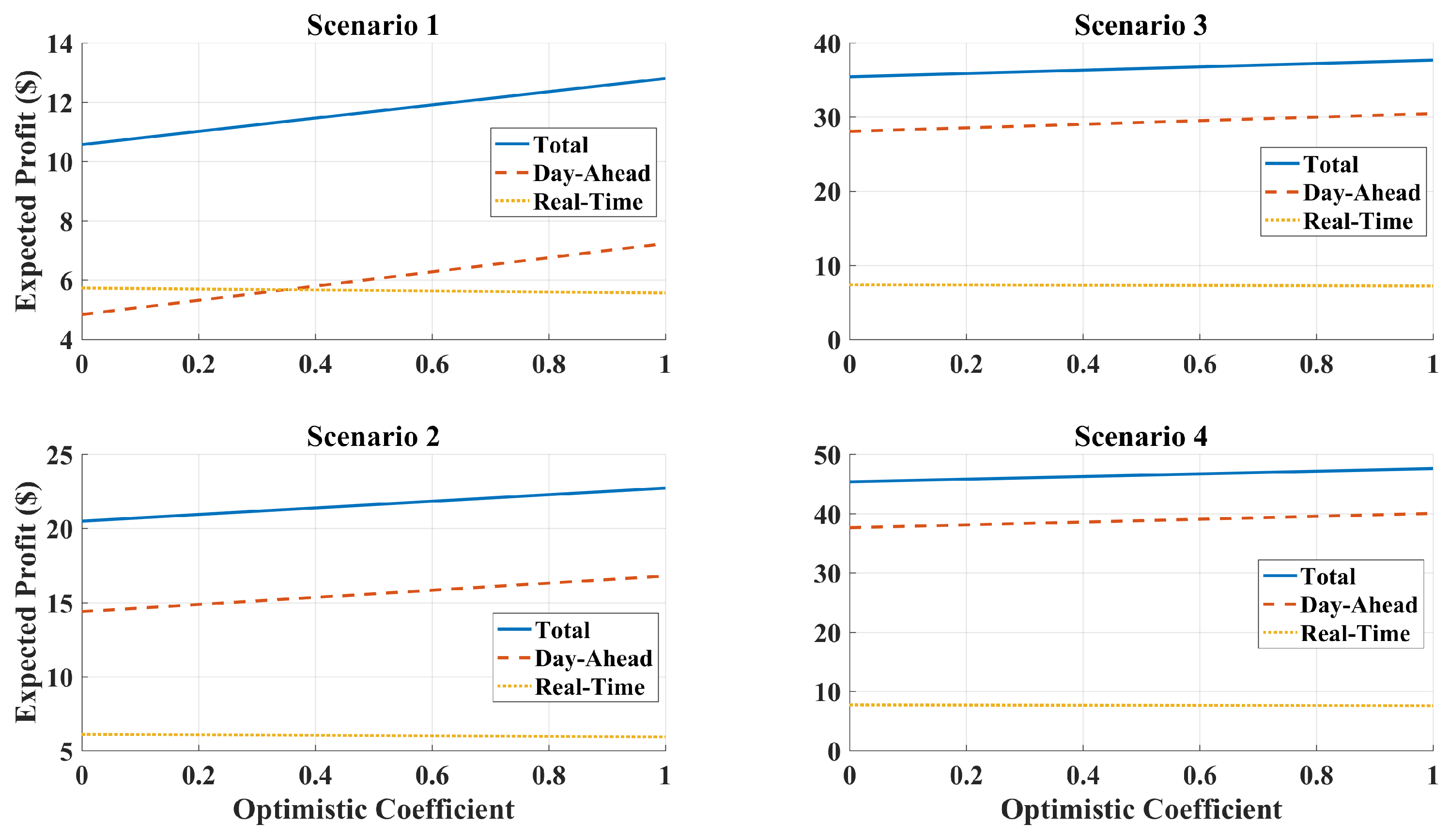
4.2. Impact of Energy Flexibility

In this section, the energy flexibility of the proposed DEMS is assessed. Hence, four scenarios are defined to analyze the performance of the system. In Scenario 1, neither the battery nor the EV are defined in the day-ahead stage of the energy management problem ( γ b a t t e r y = γ E V = 0 ). In Scenario 2, only the battery is considered in the day-ahead stage ( γ b a t t e r y = 1 , γ E V = 0 ). However, only the EV is considered in the day-ahead stage in Scenario 3 ( γ b a t t e r y = 0 , γ E V = 1 ). In Scenario 4, both (battery and EV) are modeled in the day-ahead stage ( γ b a t t e r y = γ E V = 1 ).
The impact of ESSs on the total, day-ahead and real-time expected profits of the system is shown in Figure 1. Furthermore, the influence of the optimistic coefficient, α , is evaluated in Figure 1. From this figure, it is clear that an increment of α increases the total and day-ahead expected profits because α can directly affect the power produced by the PV system through interval bands in the day-ahead stage. Hence, α increases the power generated from the PV panels in the day-ahead stage and the day-ahead expected profit. However, α has a negative impact on the amounts of the real-time expected profit. Moreover, the expected profit of the system is maximum in Scenario 4. In other words, increasing the energy flexibility of the system increases the total, day-ahead and real-time expected profits of the system. Hence, the maximum and minimum amounts of the expected profit are in Scenarios 4 and 1, respectively. Furthermore, the expected profit in Scenario 3 is more than Scenario 2 because the ramping rate of the EV is more than the battery. Therefore, the EV can provide more energy flexibility than the battery in this proposed system.

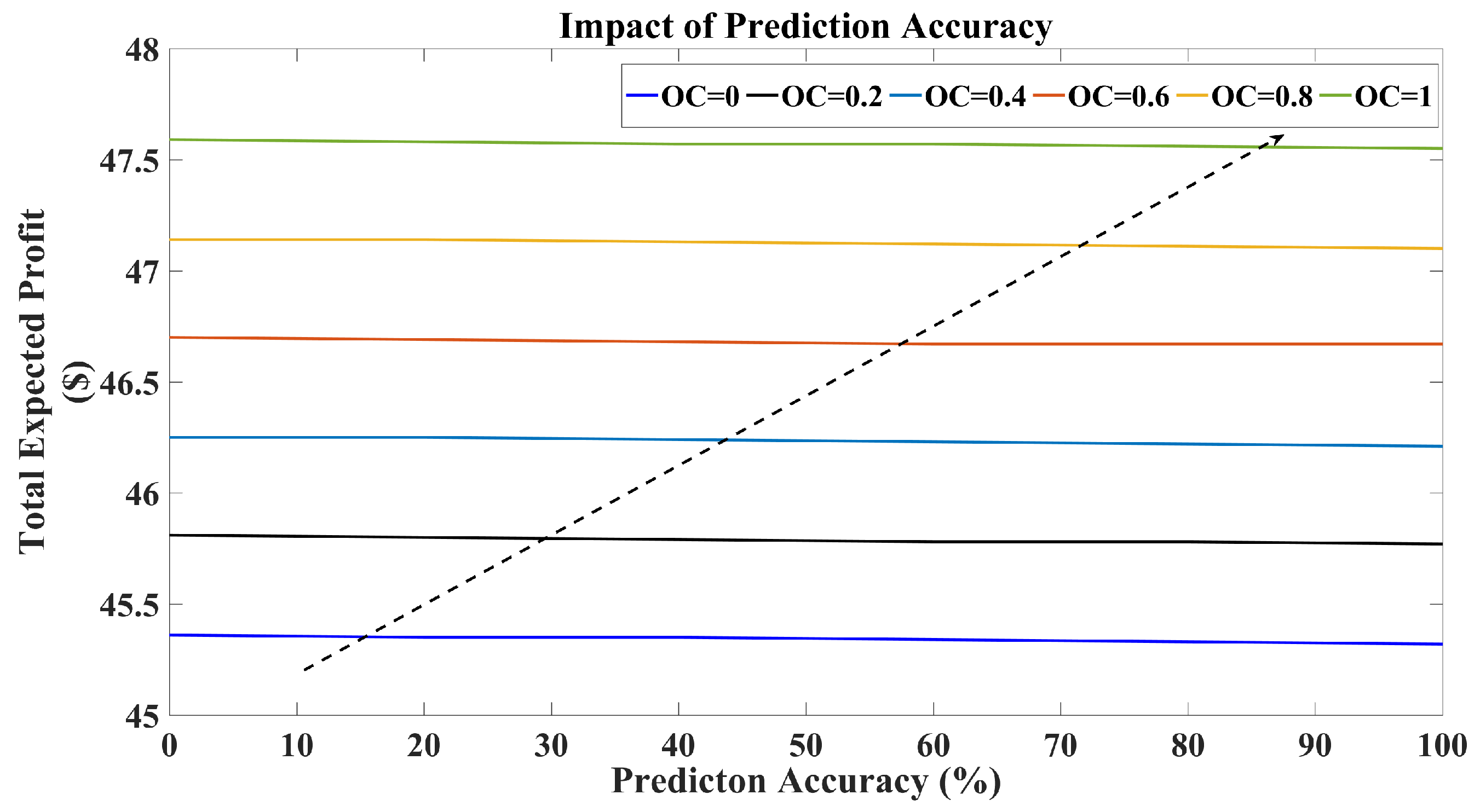
4.3. Impact of Prediction Accuracy

The prediction accuracy due to the PV power generation and its influence on the total expected profit is analyzed in this section. It is noticeable that the prediction accuracy of the outdoor temperature of the home and must-run services is considered to be 100% in this paper in order to simplify the model. Besides, it is considered that the battery and EV are modeled in the day-ahead stage in this case. As mentioned before, α increases the amount of total expected profit of the system.
According to Figure 2, the impact of the prediction accuracy on the total expected profit is evaluated based on the optimistic coefficient. Furthermore, an increase in the prediction accuracy has a smooth negative effect on the expected profit. In other words, an increment in the prediction accuracy causes a decrease of the managed power of the PV in the proposed DEMS. Hence, this decreases the expected profit of the system. According to this assessment, the maximum amount of the total expected profit of the system is where α and the prediction accuracy equal one and zero, respectively.

4.4. Impact of Demand Response

In this section, the effect of the Demand Response Program (DRP) on the EPs and the home’s electrical energy that is sold/bought to/from the local electricity market is assessed in four scenarios: with DRP, with only flexible VOLL, with only the ToU price and without DRP. Here, DRP consists of the flexible VOLL and ToU price.
As seen in Table 4, DRP causes a positive effect on the amount of total expected profit of the DEMS. In other words, while E P d a is increased when DRP is not considered in the system, E P r t is decreased because electrical loads are not flexible when DRP is not considered in the DEMS. Furthermore, The sold/bought electrical energy of the DEMS considering DRP is more/less than without considering DRP because it makes DEMS able to shift the electrical load in the time horizon of the energy management problem and reduce the loads under some conditions. However, the impact of the flexible VOLL and ToU price are not the same. Although both of them increase the sold electrical energy, the total expected profit considering only flexible VOLL is more than considering only the ToU price. This is because of the positive effect of the flexible VOLL program in the real-time stage of the DEM problem.

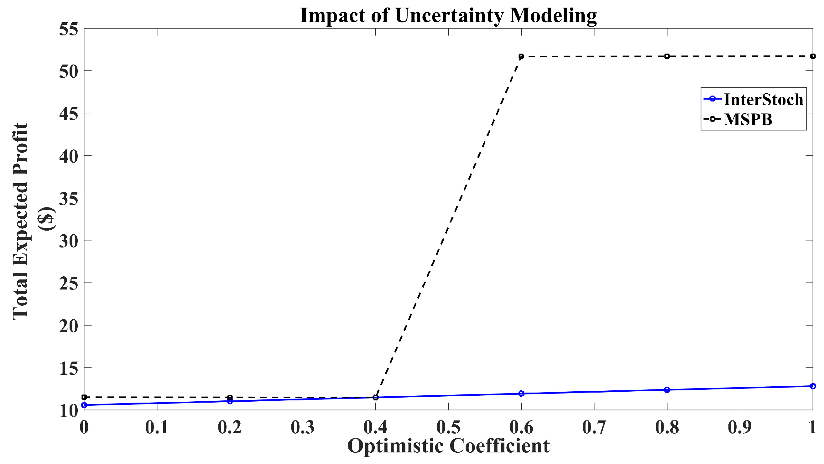
4.5. Impact of Uncertainty Modeling

In this section, the modeling of uncertainty is evaluated through a comparison of the InterStoch method and MSPB. Although the InterStoch method has been defined in this paper, MSPB has been defined in [18,19]. For simplicity, only the battery has been considered, and γ b a t t e r y is equal to zero in this section. The amounts of total, day-ahead and real-time expected profits are compared in optimistic and conservative cases based on the InterStoch and MSPB methods. As seen in Table 5, the optimistic case of both methods is where α equals one. However, the pessimistic case based on the InterStoch and MSPB methods is where α equals zero and 0.4, respectively, as seen in Table 6. Table 5 and Table 6 show that the difference between the amounts of the expected profits in the optimistic and conservative cases based on the InterStoch method is less than the MSPB method. Besides, Figure 3 shows the impact of α on the total expected profit in both methods. Figure 3 also illustrates that the worst case of the DEMS based on the InterStoch method is where α equals zero, and there is a linear pattern between the increment of the optimistic coefficient and the total expected profit when uncertainty is modeled by the InterStoch method. This point makes the system easier to analyze and more reliable, as it is able to further mitigate the uncertainty, dealing with it in away that its impact on the expected results is highly reduced. Moreover, the amount of the total expected profit in the worst case of the InterStoch is less than its amount in the worst case of the MSPB method. Hence, the InterStoch method is more robust than the MSPB method to model uncertainty in the proposed domestic energy management problem.

5. Conclusions

In this paper, the energy flexibility management of the home electricity system based on the predictive dispatch model has been introduced. Furthermore, the InterStoch hybrid method to model the uncertainty of the PV power generation has been defined for the first time in this paper. The proposed method consists of two stages. In the first stage, the day-ahead domestic energy management problem has been modeled by an interval method to consider the uncertainty due to the prediction error of PV power generation. However, a real-time problem has been represented based on the stochastic method to consider the uncertainty. The performance of the proposed domestic energy management problem has been evaluated based on a comparison between the proposed hybrid (InterStoch) and MSPB methods. Furthermore, the impact of the proposed energy flexibility model, prediction accuracy and demand response program on the expected profit and transacted electrical energy of the system and the reliability of the results has been assessed. From the simulation, it is concluded that:
  • Increasing the energy flexibility increases the total, day-ahead and real-time expected profits of the system.
  • The EV can provide more energy flexibility than the battery in the proposed system.
  • The increment of α increases the PV power produced in the day-ahead stage and day-ahead expected profit. However, α has a negative impact on the amounts of the real-time expected profit.
  • The increment of the prediction accuracy has a smooth negative impact on the expected profit.
  • For the considered case study, the demand response program has a positive effect on the amount of the DEMS’s total expected profit. Furthermore, the demand response program decreases the domestic electrical energy load.
  • The amount of the total expected profit in the worst case of InterStoch is less than its amount in the worst case of the MSPB method. Hence, the InterStoch method is more robust than the MSPB method to model uncertainty in the proposed domestic energy management problem.
Finally, it should be mentioned that the uncertainty of electrical load, the EV mobility pattern and market prices have not been modeled in our proposed DEMS. Our future work will consist of modeling the uncertainty related to the EV and must-run services and to evaluate their impacts on the transacted energy of the homes for the local electricity market.

Acknowledgments

This work has been supported by the European Commission H2020 MSCA-RISE-2014: Marie Sklodowska-Curie project DREAM-GO Enabling Demand Response for short and real-time Efficient And Market Based Smart Grid Operation—An intelligent and real-time simulation approach Ref. 641794, Grant Agreement No. 703689 (Project ADAPT) and Project SURF: Intelligent System for integrated and sustainable management of urban fleets TIN2015-65515-C4-3-R that has been supported by the Spanish Ministry, Ministerio de Economía y Competitividad and FEDER funds. Moreover, Amin Shokri Gazafroudi acknowledge the support by the Ministry of Education of the Junta de Castilla y León and the European Social Fund through a grant from predoctoral recruitment of research personnel associated with the research project "Arquitectura multiagente para la gestión eficaz de redes de energía a través del uso de técnicas de intelligencia artificial" of the University of Salamanca.

Author Contributions

Amin Shokri Gazafroudi developed the hybrid interval-stochastic method and model the residential energy management problem. Francisco Prieto-Castrillo developed the mathematical model to realize the stochastic scenarios of the system. Tiago Pinto implemented the energy management system in the test system. The remaining co-authors addressed key ideas for the project development.

Conflicts of Interest

The authors declare no conflict of interest regarding the publication of this paper.

Nomenclature

Indices
tIndex of time periods
jIndex of electrical loads
kIndex of energy storage systems
ω Index of PV power scenarios
Variables
E P Expected profit
E P d a Day-ahead expected profit
E P r t Real-time expected profit
P p v t d a Day-ahead total power generation for the PV system in period t
P p v , o u t t d a Day-ahead power generation for the PV system that is injected to the power grid in period t
P p v , i n t d a Day-ahead power generation for the PV system that is injected to the home in period t
P d i s t d a ( k ) Day-ahead total discharged power for energy storage system k in period t
P d i s , o u t t d a ( k ) Day-ahead discharged power for energy storage system k that is injected to the power grid in period t
P d i s , i n t d a ( k ) Day-ahead discharged power for energy storage system k that is injected to the home in period t
P c h t d a ( k ) Day-ahead charged power for energy storage system k that is injected to the home in period t
P n e t t d a Day-ahead power generation that is bought from the local electricity market in period t
L j t d a Day-ahead electrical load j in period t
L s h t d a Day-ahead electrical load of the space heater in period t
L s w h t d a Day-ahead electrical load of the storage water heater in period t
L p p t d a Day-ahead electrical load of the pool pump in period t
L m r s t d a Day-ahead electrical load of the must-run services in period t
C t d a ( k ) Day-ahead state of charge for energy storage system k in period t
u t d a Day-ahead discharging commitment binary variable for energy storage system k in period t
P p v t r t ( ω ) Real-time total power generation for the PV system in period t and in scenario ω
P p v , o u t t r t ( ω ) Real-time power generation for the PV system that is injected to the power grid in period t and in scenario ω
P p v , i n t r t ( ω ) Real-time power generation for the PV system that is injected to the home in period t and in scenario ω
P d i s t r t ( k , ω ) Real-time total discharged power for energy storage system k in period t and in scenario ω
P d i s , o u t t r t ( k , ω ) Real-time discharged power for energy storage system k that is injected to the power grid in period t and in scenario ω
P d i s , i n t r t ( k , ω ) Real-time discharged power for energy storage system k that is injected to the home in period t and in scenario ω
P c h t r t ( k , ω ) Real-time charged power for energy storage system k that is injected to the home in period t and in scenario ω
P n e t t r t ( ω ) Real-time power generation that is bought from local electricity market in period t and in scenario ω
L j t r t Real-time electrical load j in period t and in scenario ω
L j t s h e d ( ω ) Load shedding for load j in period t and in scenario ω
S p v t ( ω ) Spillage amount for PV in period t and in scenario ω
P p v , p t r t ( ω ) Potential power generation for PV in real time in period t and in scenario ω
L s h t r t ( ω ) Real-time electrical load of the space heater in period t and in scenario ω
L s w h t r t ( ω ) Real-time electrical load of the storage water heater in period t and in scenario ω
L p p t r t ( ω ) Real-time electrical load of the pool pump in period t and in scenario ω
L m r s t r t ( ω ) Real-time electrical load of the must-run services in period t and in scenario ω
C t r t ( k , ω ) Real-time state of charge for energy storage system k in period t and in scenario ω
u t r t ( ω ) Real-time discharging commitment binary variable for energy storage system k in period t and in scenario ω
L s h t s h e d ( ω ) Load shedding for the space heater in period t and in scenario ω
L s w h t s h e d ( ω ) Load shedding for the storage water heater in period t and in scenario ω
L p p t s h e d ( ω ) Load shedding for the pool pump in period t and in scenario ω
L m r s t s h e d ( ω ) Load shedding for the must-run services in period t and in scenario ω
θ i n t ( ω ) Indoor temperature in period t and in scenario ω
z t ( ω ) Commitment binary variable for the pool pump k in period t and in scenario ω
Parameters
P p v t p r e d Central forecasting of the PV power generation in period t
σ p v t d o w n Down deviation of the PV power prediction in period t
σ p v t u p Up deviation of the PV power prediction in period t
α p v Optimistic coefficient related to the PV power prediction
P p v t m e a n Mean of the PV power prediction in period t
Δ p v t Mean deviation of the PV power prediction in period t
π ( ω ) Probability of the PV power generation in scenario ω
λ t Sold electricity price to the local electricity market in period t
λ n e t t Bought electricity price from the local electricity market in period t
γ k Participation factor for energy storage system k
S m a x Maximum power capacity for the line
L j t p r e d Predicted electrical load j in period t
η B 2 V Charging efficiency for energy storage systems j
η V 2 B Discharging efficiency for energy storage systems j
C i Initial state of charge for energy storage systems
w m a x Maximum charging/discharging for energy storage systems
w m i n Minimum charging/discharging for energy storage systems
V O L L j Value of loss load for electrical load j
V p v s Spillage cost for the PV system
θ 0 Initial indoor temperature
θ d e s Desired indoor temperature
θ o u t t p r e d Predicted outdoor temperature
L s h m a x Maximum electrical consumption for the space heater
L s h m i n Minimum electrical consumption for the space heater
RThermal resistance of the building shell
L s w h m a x Maximum electrical consumption for the storage water heater
L s w h m i n Minimum electrical consumption for the storage water heater
U s w h Energy consumption for the storage water heater
L p p m a x Maximum electrical consumption for the pool pump
L p p m i n Minimum electrical consumption for the pool pump
T o n Maximum running hours for the pool pump
L m r s t p r e d Predicted electrical load of the must-run services in period t

References

  1. Abrishambaf, O.; Gomes, L.; Faria, P.; Afonso, J.L.; Vale, Z. Real-time simulation of renewable energy transactions in microgrid context using real hardware resources. In Proceedings of the 2016 IEEE/PES Transmission and Distribution Conference and Exposition (T&D), Dallas, TX, USA, 3–5 May 2016; pp. 1–5. [Google Scholar]
  2. Vale, Z.; Morais, H.; Faria, P.; Ramos, C. Distribution system operation supported by contextual energy resource management based on intelligent SCADA. Renew. Energy 2013, 52, 143–153. [Google Scholar] [CrossRef]
  3. Abrishambaf, O.; Ghazvini, M.A.F.; Gomes, L.; Faria, P.; Vale, Z.; Corchado, J.M. Application of a Home Energy Management System for Incentive-Based Demand Response Program Implementation. In Proceedings of the 2016 27th International Workshop on Database and Expert Systems Applications (DEXA), Porto, Portugal, 5–8 September 2016; pp. 153–157. [Google Scholar]
  4. Manic, M.; Wijayasekara, D.; Amarasinghe, K.; Rodriguez-Andina, J.J. Building Energy Management Systems The Age of Intelligent and Adaptive Buildings. IEEE Ind. Electron. Mag. 2016, 10, 25–39. [Google Scholar] [CrossRef]
  5. Shokri Gazafroudi, A.; de Paz, J.F.; Prieto-Castrillo, F.; Villarrubia, G.; Talari, S.; Shafie-khah, M.; Catalão, J.P.S. A Review of Multi-agent Based Energy Management Systems. In Proceedings of the ISAmI 2017: Ambient Intelligence—Software and Applications—8th International Symposium on Ambient Intelligence (ISAmI 2017), Porto, Portugal, 21–23 June 2017; pp. 203–209. [Google Scholar]
  6. Monteiro, V.; Pinto, J.G.; Afonso, J.L. Operation Modes for the Electric Vehicle in Smart Grids and Smart Homes: Present and Proposed Modes. IEEE Trans. Veh. Technol. 2016, 65, 1007–1020. [Google Scholar] [CrossRef] [Green Version]
  7. Zhao, C.; Dong, S.; Li, F.; Song, Y. Optimal Home Energy Management System with Mixed Types of Loads. CSEE J. Power Energy Syst. 2015, 1, 1–11. [Google Scholar] [CrossRef]
  8. Pratt, A.; Krishnamurthy, D.; Ruth, M.; Wu, H.; Lunacek, M.; Vaynshenk, P. Transactive Home Energy Management Systems: The Impact of Their Proliferation on the Electric Grid. IEEE Electrif. Mag. 2016, 4, 8–14. [Google Scholar] [CrossRef]
  9. Wang, Z.; Paranjape, R. Optimal Residential Demand Response for Multiple Heterogeneous Homes with Real-Time Price Prediction in a Multiagent Framework. IEEE Trans. Smart Grid 2017, 8, 1173–1184. [Google Scholar] [CrossRef]
  10. Paterakis, N.G.; Erdinç, O.; Bakirtzis, A.G.; Catalão, J.P.S. Optimal Household Appliances Scheduling under Day-Ahead Pricing and Load-Shaping Demand Response Strategies. IEEE Trans. Ind. Inform. 2015, 11, 1509–1519. [Google Scholar] [CrossRef]
  11. Erdinc, O.; Paterakis, N.G.; Mendes, T.D.P.; Bakirtzis, A.G.; Catalão, J.P.S. Smart Household Operation Considering Bi-Directional EV and ESS Utilization by Real-Time Pricing-Based DR. IEEE Trans. Smart Grid 2015, 6, 1281–1291. [Google Scholar] [CrossRef]
  12. Sarker, M.R.; Ortega-Vazquez, M.A.; Kirschen, D.S. Optimal Coordination and Scheduling of Demand Response via Monetary Incentives. IEEE Trans. Smart Grid 2015, 6, 1341–1352. [Google Scholar] [CrossRef]
  13. Althaher, S.; Mancarella, P.; Mutale, J. Automated Demand Response From Home Energy Management System Under Dynamic Pricing and Power and Comfort Constraints. IEEE Trans. Smart Grid 2015, 6, 1874–1883. [Google Scholar] [CrossRef]
  14. Althaher, S.; Mancarella, P.; Mutale, J. Equivalence of Multi-Time Scale Optimization for Home Energy Management Considering User Discomfort Preference. IEEE Trans. Smart Grid 2017, 8, 1876–1887. [Google Scholar]
  15. Huang, Y.; Wang, L.; Guo, W.; Kang, Q.; Wu, Q. Chance Constrained Optimization in a Home Energy Management System. IEEE Trans. Smart Grid 2016, PP, 1-1. [Google Scholar] [CrossRef]
  16. Yoon, S.; Choi, Y.; Park, J.; Bahk, S. Stackelberg Game based Demand Response for At-Home Electric Vehicle Charging. IEEE Trans. Veh. Technol. 2016, 65, 4172–4184. [Google Scholar] [CrossRef]
  17. Wu, X.; Hu, X.; Yi, X.; Moura, S. Stochastic Optimal Energy Management of Smart Home with PEV Energy Storage. IEEE Trans. Smart Grid 2016, PP, 1-1. [Google Scholar] [CrossRef]
  18. Shokri Gazafroudi, A.; Pinto, T.; Prieto-Castrillo, F.; Prieto, J.; Corchado, J.M.; Jozi, A.; Vale, Z.; Venayagamoorthy, G.K. Organization-based Multi-Agent Structure of the Smart Home Electricity System. In Proceedings of the 2017 IEEE Congress on Evolutionary Computation (CEC), San Sebastian, Spain, 5–8 June 2017. [Google Scholar]
  19. Shokri Gazafroudi, A.; Prieto-Castrillo, F.; Corchado, J.M. Residential Energy Management Using a Novel Interval Optimization Method. In Proceedings of the 4th International Conference on Control, Decision and Information Technology 2017 (CoDIT 2017), Barcelona, Spain, 5–8 April 2017. [Google Scholar]
  20. GAMS Release 2.50. A User’s Guide. GAMS Development Corporation, 1999. Available online: http://www.gams.com (accessed on 2 August 2017).
Figure 1. Impact of energy flexibility on the amounts of total, day-ahead and real-time expected profits.
Energies 10 01397 g001
Figure 2. Impact of prediction accuracy on the total expected profit of the system. OC, Optimistic Coefficient.
Energies 10 01397 g002
Figure 3. Impact of uncertainty modeling on the total expected profit of the system.
Energies 10 01397 g003
Table 1. Predicted data of uncertain variables [18].
t P pv t pred (kW) σ pv down (kW) σ pv up (kW) θ out t pred ( C) L mrs t pred (kW)
100.000.005.50.005
200.000.005.50.005
300.000.005.20.005
400.000.005.20.005
500.000.004.80.005
600.000.005.50.005
70.100.010.026.50.005
80.200.020.047.50.005
90.420.030.079.80.005
100.760.080.26100.005
111.10.120.23110.005
121.320.130.26120.005
131.910.100.19120.005
140.850.020.04120.005
150.290.020.04110.005
160.310.020.03100.005
170.060.010.0190.005
1800.000.008.50.005
1900.000.0080.005
2000.000.007.51.218
2100.000.0070.262
2200.000.006.50.14
2300.000.006.20.127
2400.000.0060.005
Table 2. ToU Price data of the system.
Time (hour)Price ($/MW)
λ i λ net
23–72.20.0814
8–142.20.1408
15–202.20.3564
21–222.20.1408
Table 3. Value of Loss Load (VOLL) and spillage costs. SH, Space Heater; SWH, Storage Water Heater; PP, Pool Pump.
Time (hour)VOLL ($/MW)Spillage Cost ($/MW)
SHSWHPPMRSPV
22–711 0.5 2.24
8–21110.252.24
Table 4. Impact of demand response program on the amount of expected profit of the system and sold/bought electrical energy to/from the local electricity market. DRP, Demand Response Program.
Demand Response Scenarios α = 1
EP total EP da EP rt E sold E bought
With DRP (Flexible VOLL + ToU)47.57140.0037.56818.60543.033
With Only Flexible VOLL47.77542.4095.36514.40637.995
With Only ToU Price42.07140.0032.06815.23649.432
Without DRP42.27540.409 0.135 13.84747.842
Table 5. Impact of uncertainty modeling on day-ahead, real time and total expected profits under the optimistic case. InterStoch, Interval-Stochastic; MSPB, Modified Stochastic Predicted Band.
Expected Profit ($)InterStoch ( α = 1)MSPB ( α = 1)
With UncertaintyWithout UncertaintyWith UncertaintyWithout Uncertainty
E P t o t a l 12.79810.54951.70751.618
E P d a 7.2344.83649.23249.232
E P r t 5.5645.7132.4752.386
Table 6. Impact of uncertainty modeling on day-ahead, real time and total expected profits under the conservative case.
Expected Profit ($)InterStoch ( α = 0)MSPB ( α = 0.4)
With UncertaintyWithout UncertaintyWith UncertaintyWithout Uncertainty
E P t o t a l 10.56910.54911.44951.618
E P d a 4.8364.8364.83649.232
E P r t 5.7335.7136.6132.386

