Stability of DC Distribution Systems: An Algebraic Derivation

Abstract

Instability caused by low inertia and constant power loads is a major challenge of DC distribution grids. Previous research uses oversimplified models or does not provide general rules for stability. Therefore, a comprehensive approach to analyze the stability of DC distribution systems is desired. This paper presents a method to algebraically analyze the stability of any DC distribution system through the eigenvalues of its state-space matrices. Furthermore, using this method, requirements are found for the stability of three example systems. Additionally, a sensitivity analysis is performed, which considers the effect of several system parameters on the stability and disputes some overgeneralized conclusions of previous research. Moreover, various simulations are performed to illustrate the dynamic behavior of a stable and an unstable DC distribution system.

1. Introduction

The adoption of DC distribution systems is growing rapidly. The utilization of DC distribution systems for applications such as high voltage distribution [1,2], data centers [2,3], telecommunications [4], commercial [5,6] and residential buildings [7,8,9], and street lighting [10,11] is ever increasing. Moreover, a variety of novel applications, such as microgrids and device level distribution, have recently been identified [12,13].

A challenge for future distribution grids is instability, which is caused by the (anticipated) low inertia of future grids and the interaction between power electronic converters. Conventional generation provides (virtual) inertia to the grid by naturally governing the kinetic energy of its angular mass or via the control of its power electronic converter. With the increasing share of renewable (distributed) energy sources, this (virtual) inertia of distribution grids is decreased significantly [14]. Moreover, tightly regulated load converters behave as constant power loads (CPLs). Constant power loads exhibit a negative incremental input impedance, which has a destabilizing effect on distribution systems [15].

Two current methods have been identified to counteract instability caused by CPLs in DC distribution systems. First, passive stabilization methods utilize passive elements (e.g., resistance, filters or storage) to dampen the oscillations in the system [16,17]. However, passive stabilization methods increase the cost, complexity and losses of the system. Second, active stabilization methods utilize advanced control methods to improve stability. Examples of different active stabilization techniques can be found in literature [18,19]. However, it is more appealing to ensure inherent stability (if possible).

To analyze the stability of DC distribution systems, several models of the network and converters have been reported in literature. Most methods average and linearize the power electronic converters in the DC distribution grid. Since these small-signal models are valid for frequencies up to half of the switching frequencies, and the bandwidths of practical converters are typically lower than one-tenth of the switching frequency, these models provide reasonable accuracy around the operating point [18].

Four main approaches to the stability analysis of DC distribution grids can be identified. Firstly, the minor loop gain (the relationship between the complex load and source impedance) can be analyzed. Different limits on the minor loop gain have been proposed to ensure stability. However, this approach assumes unidirectional power flow and measurements are essential for accurate impedance estimations [18,20,21,22]. Secondly, a root locus analysis of the system can be performed and the locations of the poles can be analyzed [23,24,25,26,27]. This approach does not provide rules for stability and often provides little (mathematical) insight into the origin of the (in)stability. Thirdly, an analysis based on Lyapunov methods can be conducted [28,29,30,31,32]. However, these are not easily applied and require a suitable construction of the Lyapunov storage function. Lastly, the roots of the system can be derived from the eigenvalues of its state-space matrix [19,33,34,35,36]. This approach, which is also used in this paper, relies on the validity of averaging, linearizing, and simplifying the power electronic converter.

Previous research, however, only analyzes specific systems, uses oversimplified models and/or does not provide general rules for stability. For example, only star type systems with a source at the central node are analyzed [35], the node capacitance is not considered in the equations [37], or no (general) rules for stability are provided [25]. Therefore, any conclusions on the effect of system parameters (e.g., inductance, capacitance and droop coefficients) on the distribution system’s stability can not be generalized.

The contribution of this paper is a generalized method to algebraically analyze the stability of DC distribution systems, regardless of configuration. The method derives necessary and sufficient conditions for the stability by determining the system’s eigenvalues algebraically. Furthermore, the presented model is used to prove and refute some of the common conclusions on the effect of certain system parameters on stability.

The remainder of this paper is organized as follows: in Section 2, the model which is used for each component is described. Section 3 discusses the stability of the simplest DC distribution systems. A method to analyze the stability of any DC distribution grid is presented in Section 4. Subsequently, in Section 5, the presented method is applied to three different examples. Section 6 illustrates the stable and unstable dynamic behavior of DC distribution grids via various simulations. Finally, conclusions are drawn in Section 7.

2. DC Distribution System Model

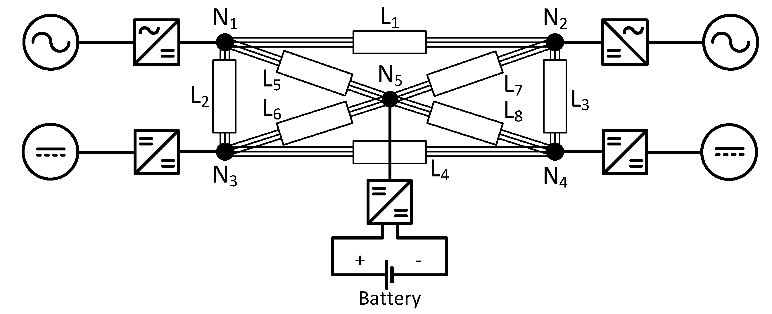
In Figure 1, an example of a DC distribution system is shown. Any DC distribution system consists of n nodes, l distribution lines, o phase conductors, and m sources and loads connected to nodes via power electronic converters. For the sake of simplicity, the DC distribution systems in this paper are assumed to be monopolar (i.e., have a single phase conductor), but the model can be extended. The interconnectivity of the system can then be described by the incidence matrix $\mathbf{\Gamma }$ [38]:

$$\mathbf{\Gamma }(j,i)=\left\{\begin{array}{cc}1,\hfill & \mathrm{if}{I}_j\mathrm{is}\mathrm{flowing}\mathrm{from}\mathrm{node}i,\hfill \\ -1,\hfill & \mathrm{if}{I}_j\mathrm{is}\mathrm{flowing}\mathrm{in}\mathrm{node}i,\hfill \\ 0,\hfill & \mathrm{otherwise},\hfill \end{array}\right.$$

(1)

where j and i are the indices for each distribution line and node, respectively, and $I_j$ is the current flowing in line j. Furthermore, the boldface of a variable indicates that it is a vector or matrix.

2.1. Nodes

The voltages at the system’s nodes are determined by the set of differential equations

$$\begin{array}{cc}\hfill \mathit{C}{\dot{\mathit{U}}}_{\mathit{N}}& ={\mathit{I}}_{\mathit{M}}-{\mathbf{\Gamma }}^{\mathit{T}}{\mathit{I}}_{\mathit{L}},\hfill \end{array}$$

(2)

where $\mathit{C}$ is the (diagonal) capacitance matrix, ${\mathit{U}}_{\mathit{N}}$ are the voltages at each node, ${\mathit{I}}_{\mathit{L}}$ are the currents in each distribution line, and ${\mathit{I}}_{\mathit{M}}$ are the sums of the currents from the converters connected to each node.

2.2. Distribution Lines

The currents in the system’s distribution lines are determined by the set of differential equations

$$\begin{array}{cc}\hfill \mathit{L}{\dot{\mathit{I}}}_{\mathit{L}}& =\mathbf{\Gamma }{\mathit{U}}_{\mathit{N}}-{\mathit{RI}}_{\mathit{L}},\hfill \end{array}$$

(3)

where $\mathit{L}$ and $\mathit{R}$ are the (diagonal) inductance and resistance matrices, respectively.

2.3. Sources

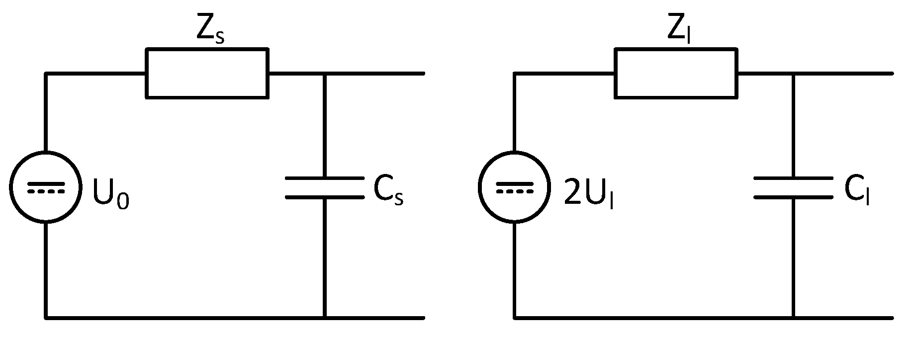
It is assumed that the source and load converters have a large enough bandwidth that they react instantaneously to changes in the system. The equivalent circuits of droop controlled sources and constant power loads are given in Figure 2. The current flowing from a droop controlled source into a node is then

$$\begin{array}{cc}\hfill I_s& =\frac{U_0-U_n}{Z_s},\hfill \end{array}$$

(4)

where $U_0$ is the reference voltage, $U_n$ is the node voltage, and $Z_s$ is the (virtual) impedance of the droop controller.

2.4. Loads

The linearized load current of constant power loads, assuming a large enough bandwidth of the converter, is

$$\begin{array}{c}\hfill I_l=-\frac{2P_l}{U_l}+\frac{P_l}{U_l^2}{U}_n=\frac{2U_l-U_n}{Z_l}=I_0-\frac{U_n}{Z_l},\end{array}$$

(5)

where

$$Z_l=-\frac{U_l^2}{P_l},$$

(6)

$P_l$ is the load’s power, $U_l$ is the voltage at which the load is linearized, and $Z_l$ is the (negative) impedance of the load [26].

3. Stability of Simple DC Distribution Systems

The simplest (potentially unstable) DC distribution grid is a voltage source connected to a constant power load via a distribution line, which is shown in Figure 3. The differential equations of this system are

$$\begin{array}{cc}\hfill C{\dot{U}}_C& =I_L+I_l,\hfill \end{array}$$

(7)

$$\begin{array}{cc}\hfill L{\dot{I}}_L& =U_S-U_C-R{I}_L,\hfill \end{array}$$

(8)

where $U_C$ is the voltage of the capacitor and $I_L$ is the current flowing in the inductor. By substituting Equation (5) into the differential equations, the state-space formulation is derived to be

$$\left[\begin{array}{c}{\dot{U}}_C\\ {\dot{I}}_L\end{array}\right]=\left[\begin{array}{cc}\frac{-1}{Z_{l}C}& \frac{1}{C}\\ -\frac{1}{L}& -\frac{R}{L}\end{array}\right]\left[\begin{array}{c}{U}_C\\ I_L\end{array}\right]+\left[\begin{array}{cc}\frac{1}{C}& 0\\ 0& \frac{1}{L}\end{array}\right]\left[\begin{array}{c}{I}_0\\ U_S\end{array}\right].$$

(9)

The poles of any state-space system can be found by determining the eigenvalues of the “$\mathit{A}$” matrix (the left matrix in Equation (9)). In fact, the eigenvalues of this matrix can be found by solving $|\mathit{A}-\lambda \mathit{I}|=0$. The characteristic equation ($|\mathit{A}-\lambda \mathit{I}|$) of this system is

$${\lambda }^2+\lambda \left(\frac{R}{L}+\frac{1}{C{Z}_l}\right)+\frac{1}{LC}+\frac{R}{LC{Z}_l}.$$

(10)

Therefore, the poles of this system are

$$\begin{array}{cc}\hfill \lambda =& -\frac{R}{2L}-\frac{1}{2C{Z}_l}\pm \sqrt{\frac{1}{4}{\left(\frac{R}{L}+\frac{1}{C{Z}_l}\right)}^2-\left(\frac{1}{LC}+\frac{R}{LC{Z}_l}\right)}.\hfill \end{array}$$

(11)

Any system is considered stable if all poles have negative real parts. Consequently, this system is stable if and only if

$$\begin{array}{cc}\hfill \frac{R}{L}+\frac{1}{C{Z}_l}& >0,\hfill \end{array}$$

(12)

$$\begin{array}{cc}\hfill \frac{1}{R}+\frac{1}{Z_l}& >0.\hfill \end{array}$$

(13)

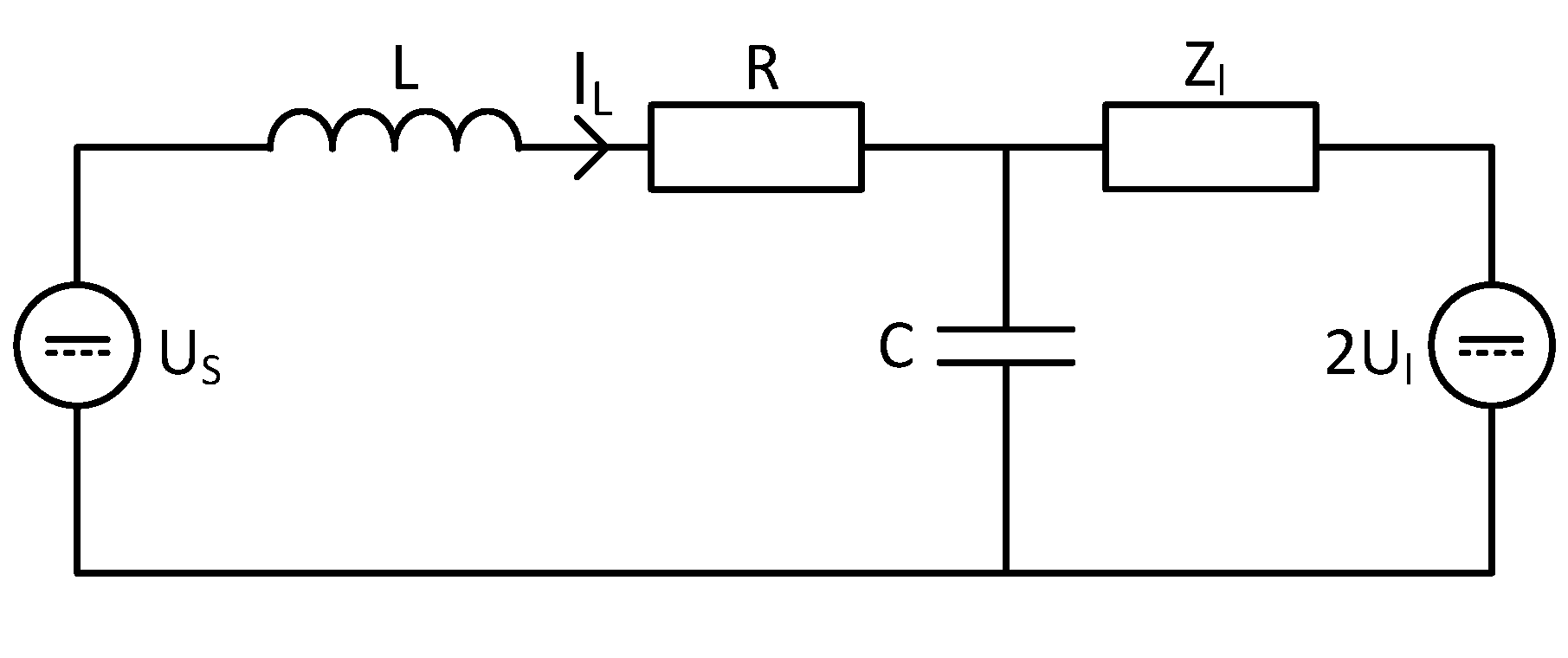
A slightly more complex DC distribution grid is given in Figure 4, where the voltage source of the previous example is replaced by a droop controlled source. To generalize droop controlled sources and constant power loads, the current flowing from any converter into the node it is connected to is given by

$$I_i=I_{i,0}-\frac{1}{Z_i}{U}_C,$$

(14)

where $I_{i,0}$ and $Z_i$ are positive for droop controlled sources, and negative for constant power loads. The state-space formulation of this DC distribution system is then

$$\left[\begin{array}{c}{\dot{U}}_1\\ {\dot{U}}_2\\ {\dot{I}}_L\end{array}\right]=\left[\begin{array}{ccc}\frac{-1}{Z_1{C}_1}& 0& \frac{-1}{C_1}\\ 0& \frac{-1}{Z_2{C}_2}& \frac{1}{C_2}\\ \frac{1}{L}& \frac{-1}{L}& \frac{-R}{L}\end{array}\right]\left[\begin{array}{c}{U}_1\\ U_2\\ I_L\end{array}\right]+\left[\begin{array}{cc}\frac{1}{C_1}& 0\\ 0& \frac{1}{C_2}\\ 0& 0\end{array}\right]\left[\begin{array}{c}{I}_{1,0}\\ I_{2,0}\end{array}\right].$$

(15)

Once again, the characteristic equation is derived by determining $|\mathit{A}-\lambda \mathit{I}|$:

$$\begin{array}{c}{\lambda }^3+{\lambda }^2\left(\frac{R}{L}+\frac{1}{C_1{Z}_1}+\frac{1}{C_2{Z}_2}\right)+\hfill \\ \lambda \frac{1}{L{C}_1{C}_2}\left(\frac{L}{Z_1{Z}_2}+\frac{C_{2}R}{Z_1}+\frac{C_{1}R}{Z_2}+C_2+C_1\right)+\hfill \\ \frac{1}{L{C}_1{C}_2}\left(\frac{R}{Z_1{Z}_2}+\frac{1}{Z_1}+\frac{1}{Z_2}\right).\hfill \end{array}$$

(16)

It is required, but not sufficient, that all coefficients of a polynomial are positive for it to have only poles with negative real parts; therefore,

$$\begin{array}{cc}\hfill \frac{R}{L}+\frac{1}{C_1{Z}_1}+\frac{1}{C_2{Z}_2}& >0,\hfill \end{array}$$

(17)

$$\begin{array}{cc}\hfill \frac{L}{Z_1{Z}_2}+\frac{C_{2}R}{Z_1}+\frac{C_{1}R}{Z_2}+C_2+C_1& >0,\hfill \end{array}$$

(18)

$$\begin{array}{cc}\hfill \frac{R}{Z_1{Z}_2}+\frac{1}{Z_1}+\frac{1}{Z_2}& >0.\hfill \end{array}$$

(19)

To make the conditions sufficient, in this third order case, one additional condition (that the product of the second and third coefficients is greater than the fourth) is required.

If, for the sake of simplicity, the resistance (R) is neglected and the source is located at node 1, the system presented in Figure 4 is stable if and only if

$$\begin{array}{cc}\hfill \left|Z_2\right|& >\left|Z_1\right|,\hfill \end{array}$$

(20)

$$\begin{array}{cc}\hfill C_2\left|Z_2\right|& >C_1\left|Z_1\right|,\hfill \end{array}$$

(21)

$$\begin{array}{cc}\hfill C_2+C_1& >\frac{L}{\left|Z_1{Z}_2\right|},\hfill \end{array}$$

(22)

$$\begin{array}{cc}\hfill \frac{L}{C_2{Z}_1{Z}_2^2}+\frac{C_2}{C_1{Z}_1}& >\frac{L}{C_1{Z}_1^2\left|Z_2\right|}+\frac{C_1}{C_2\left|Z_2\right|}.\hfill \end{array}$$

(23)

4. Stability of Any DC Distribution System

The approach used in the previous section is in this section extended for any DC distribution system. By combining Equations (2), (3) and (14) the state-space formulation for any DC distribution consisting of nodes, distribution lines, droop controlled sources and (constant power) loads is derived to be

$$\begin{array}{c}\hfill \left[\begin{array}{c}\dot{{\mathit{U}}_{\mathit{N}}}\\ \dot{{\mathit{I}}_{\mathit{L}}}\end{array}\right]=\left[\begin{array}{cc}-{\mathit{C}}^{-1}{\mathit{Z}}^{-1}& -{\mathit{C}}^{-1}{\Gamma }^{\mathit{T}}\\ {\mathit{L}}^{-1}\Gamma & -{\mathit{L}}^{-1}\mathit{R}\end{array}\right]\left[\begin{array}{c}{\mathit{U}}_{\mathit{N}}\\ {\mathit{I}}_{\mathit{L}}\end{array}\right]+\left[\begin{array}{c}{\mathit{C}}^{-1}\\ \varnothing \end{array}\right]{\mathit{I}}_{\mathit{M},\mathbf{0}},\end{array}$$

(24)

where $\mathit{Z}$ is the matrix containing source and load impedance and ${\mathit{I}}_{\mathit{M},\mathbf{0}}$ is the vector of the constant term currents ($I_{i,0}$) from the converters connected to each node.

4.1. The Location of the Equilibrium

Besides the stability, the equilibrium (steady state) of the system can be derived from the state-space equations. In steady state, the time derivatives in the system are 0. The steady state voltages and currents can therefore be calculated by

$$\begin{array}{cc}\hfill \varnothing & =\left[\begin{array}{cc}-{\mathit{C}}^{-1}{\mathit{Z}}^{-1}& -{\mathit{C}}^{-1}{\Gamma }^{\mathit{T}}\\ {\mathit{L}}^{-1}\Gamma & -{\mathit{L}}^{-1}\mathit{R}\end{array}\right]\left[\begin{array}{c}{\mathit{U}}_{\mathit{N}}\\ {\mathit{I}}_{\mathit{L}}\end{array}\right]+\left[\begin{array}{c}{\mathit{C}}^{-1}\\ \varnothing \end{array}\right]{\mathit{I}}_{\mathit{M},\mathbf{0}},\hfill \end{array}$$

(25)

$$\begin{array}{cc}\hfill \left[\begin{array}{c}{\mathit{U}}_{\mathit{N}}\\ {\mathit{I}}_{\mathit{L}}\end{array}\right]& ={\left[\begin{array}{cc}-{\mathit{C}}^{-1}{\mathit{Z}}^{-1}& -{\mathit{C}}^{-1}{\Gamma }^{\mathit{T}}\\ {\mathit{L}}^{-1}\Gamma & -{\mathit{L}}^{-1}\mathit{R}\end{array}\right]}^{-1}\left[\begin{array}{c}-{\mathit{C}}^{-1}\\ \varnothing \end{array}\right]{\mathit{I}}_{\mathit{M},\mathbf{0}}.\hfill \end{array}$$

(26)

The inverse of the left-hand matrix ($\mathit{A}$) can be decomposed as

$${\mathit{A}}^{-1}={\left[\begin{array}{cc}{\mathit{Z}}^{-1}& {\mathbf{\Gamma }}^{\mathit{T}}\\ \mathbf{\Gamma }& -\mathit{R}\end{array}\right]}^{-1}\left[\begin{array}{cc}-\mathit{C}& 0\\ 0& \mathit{L}\end{array}\right].$$

(27)

By substituting Equation (27) into Equation (26), the steady state node voltages and line currents are derived to be

$$\begin{array}{c}\hfill \left[\begin{array}{c}{\mathit{U}}_{\mathit{N}}\\ {\mathit{I}}_{\mathit{L}}\end{array}\right]={\left[\begin{array}{cc}{\mathit{Z}}^{-1}& {\mathbf{\Gamma }}^{\mathit{T}}\\ \mathbf{\Gamma }& -\mathit{R}\end{array}\right]}^{-1}\left[\begin{array}{c}{\mathit{I}}_{\mathit{M},\mathbf{0}}\\ \varnothing \end{array}\right].\end{array}$$

(28)

Since the matrix of Equation (28) is a block matrix, the node voltages at the equilibrium are

$$\begin{array}{cc}\hfill {\mathit{U}}_{\mathit{N}}& ={({\mathit{Z}}^{-1}+{\mathbf{\Gamma }}^{\mathit{T}}{\mathit{R}}^{-1}\mathbf{\Gamma })}^{-1}{\mathit{I}}_{\mathit{M},\mathbf{0}},\hfill \end{array}$$

(29)

which is equivalent to multiplying the constant term currents by the equivalent impedance of the network.

4.2. Stability from the Characteristic Equation

The stability of DC distribution systems can be evaluated by determining the eigenvalues of the $\mathit{A}$ matrix. For the ease of computation, this matrix is represented by

$$\mathit{A}=\left[\begin{array}{cc}-{\mathit{C}}^{-1}{\mathit{Z}}^{-1}& -{\mathit{C}}^{-1}{\mathbf{\Gamma }}^{\mathit{T}}\\ {\mathit{L}}^{-1}\mathbf{\Gamma }& -{\mathit{L}}^{-1}\mathit{R}\end{array}\right]=\left[\begin{array}{cc}\mathit{E}& \mathit{F}\\ \mathit{G}& \mathit{H}\end{array}\right],$$

(30)

where $\mathit{F}$ and $\mathit{G}$ are not necessarily square matrices.

The characteristic equation of this matrix ($|\mathit{A}-\lambda \mathit{I}|$) will always have the form of

$$a_1{\lambda }^{N+L}+a_2{\lambda }^{N+L-1}+a_3{\lambda }^{N+L-2}\cdots a_{N+L}=0,$$

(31)

where N and L are the number of nodes and number of distribution lines, respectively. Therefore, this characteristic equation has $N+L$ coefficients and $N+L$ zeros.

The coefficients of the characteristic equation can be determined from the $\mathit{A}$ matrix by utilizing traces of powers or the principal minors of the matrix [39,40]:

$$\begin{array}{cc}\hfill a_1& =1,\hfill \end{array}$$

(32)

$$\begin{array}{cc}\hfill a_{1+k}& =-\frac{1}{k}\sum _{m=1}^{m=k}{a}_{m}Tr\left({\mathit{A}}^{k-m+1}\right),\hfill \end{array}$$

(33)

$$\begin{array}{cc}\hfill a_{1+k}& ={(-1)}^k\sum {\Delta }_k,\hfill \end{array}$$

(34)

where Tr is the trace of a matrix, and ${\Delta }_k$ is the k-th order principal minor of $\mathit{A}$.

Utilizing Equations (33) and (30), the algebraic representation of the first five coefficients of the characteristic equation are determined to be

$$\begin{array}{cc}\hfill a_1=& 1,\hfill \end{array}$$

(35)

$$\begin{array}{cc}\hfill a_2=& -\sum _i{\mathit{A}}_{ii},\hfill \end{array}$$

(36)

$$\begin{array}{cc}\hfill a_3=& \frac{1}{2}\sum _{i\ne j}{\mathit{A}}_{ii}{\mathit{A}}_{jj}-\sum _i{\left(\mathit{F}\mathit{G}\right)}_{ii},\hfill \end{array}$$

(37)

$$\begin{array}{cc}\hfill a_4=& -\frac{1}{6}\sum _{i\ne j\ne k}{\mathit{A}}_{ii}{\mathit{A}}_{jj}{\mathit{A}}_{kk}\hfill \\ \hfill & +\frac{1}{2}\sum _{i\ne j}{\mathit{E}}_{ii}{\left(\mathit{F}\mathit{G}\right)}_{jj}+\frac{1}{2}\sum _{i\ne j}{\mathit{H}}_{ii}{\left(\mathit{G}\mathit{F}\right)}_{jj},\hfill \end{array}$$

(38)

$$\begin{array}{cc}\hfill a_5=& \frac{1}{24}\sum _{i\ne j\ne k\ne l}{\mathit{A}}_{ii}{\mathit{A}}_{jj}{\mathit{A}}_{kk}{\mathit{A}}_{ll}\hfill \\ \hfill & -\frac{1}{6}\sum _{i\ne j\ne k}{\mathit{E}}_{ii}{\mathit{E}}_{jj}{\left(\mathit{F}\mathit{G}\right)}_{kk}-\frac{1}{6}\sum _{i\ne j\ne k}{\mathit{H}}_{ii}{\mathit{H}}_{jj}{\left(\mathit{G}\mathit{F}\right)}_{kk}\hfill \\ \hfill & -\frac{1}{6}\sum {\mathit{E}}_{ii}{\mathit{H}}_{jj}{\left(\mathit{F}\mathit{G}\right)}_{kk}\hfill \\ \hfill & -\frac{1}{2}\sum {\left(\mathit{E}\mathit{F}\mathit{H}\mathit{G}\right)}_{ii}-\frac{1}{2}\sum {\left(\mathit{H}\mathit{G}\mathit{E}\mathit{F}\right)}_{ii}\hfill \\ \hfill & +\frac{1}{2}\sum {\mathit{E}}_{ii}{\left(\mathit{F}\mathit{H}\mathit{G}\right)}_{jj}+\frac{1}{2}\sum {\mathit{H}}_{ii}{\left(\mathit{G}\mathit{E}\mathit{F}\right)}_{jj}\hfill \\ \hfill & -\frac{1}{2}\sum {\left(\mathit{F}\mathit{G}\right)}_{ii}^2+\frac{1}{4}\sum {\left(\mathit{F}\mathit{G}\right)}_{ii}{\left(\mathit{F}\mathit{G}\right)}_{jj}.\hfill \end{array}$$

(39)

From Equations (35) to (39), it becomes apparent that the coefficients relate to the combinations of the sources’, loads’ and distribution lines’ time coefficients, of increasing order with each subsequent coefficient (without creating loops).

For these systems to be stable, it is required, but not sufficient, that all coefficients are larger than 0 [41]. To make the conditions sufficient $(N+L-2)$ additional coefficients need to be added [42]. These Routh coefficients can be found in the leftmost column of the Routh array [42]:

$$B=\left[\begin{array}{ccccc}{a}_1& a_3& a_5& \cdots & a_x\\ a_2& a_4& a_6& \cdots & a_x\\ b_{1,1}& b_{1,2}& b_{1,3}& \cdots & b_{1,x/2}\\ b_{2,1}& b_{2,2}& b_{2,3}& \cdots & b_{2,x/2}\\ ⋮& ⋮& ⋮& ⋮& ⋮\\ b_{x-2,1}& b_{x-2,2}& b_{x-2,3}& \cdots & b_{x-2,x/2}\end{array}\right],$$

(40)

where x is equal to $N+L$, and the $b_{i,j}$ elements are recursively determined by

$$b_{i,j}=\frac{B_{1+i,1}{B}_{i,1+j}-B_{i,1}{B}_{1+i,1+j}}{B_{1+i,1}}.$$

(41)

For example, the first two Routh coefficients are

$$\begin{array}{cc}\hfill b_{1,1}& =a_2{a}_3-a_4,\hfill \end{array}$$

(42)

$$\begin{array}{cc}\hfill b_{2,1}& =a_2{a}_3{a}_4+a_2{a}_6-a_2^2{a}_5-a_4^2.\hfill \end{array}$$

(43)

Any DC distribution system is stable if and only if all the coefficients of the characteristic equation and the Routh coefficients ($b_{1,j}$) are larger than zero.

5. Stability Analysis of Example Systems

To demonstrate the utility of the presented method, the stability of three DC distribution systems in different configurations is analyzed. For these examples, it is assumed that the source is located at node $N_1$ of each configuration; however, moving the source to a different node yields similar results. Furthermore, a sensitivity analysis is performed and a few general misconceptions concerning the stability of DC distribution systems are discussed.

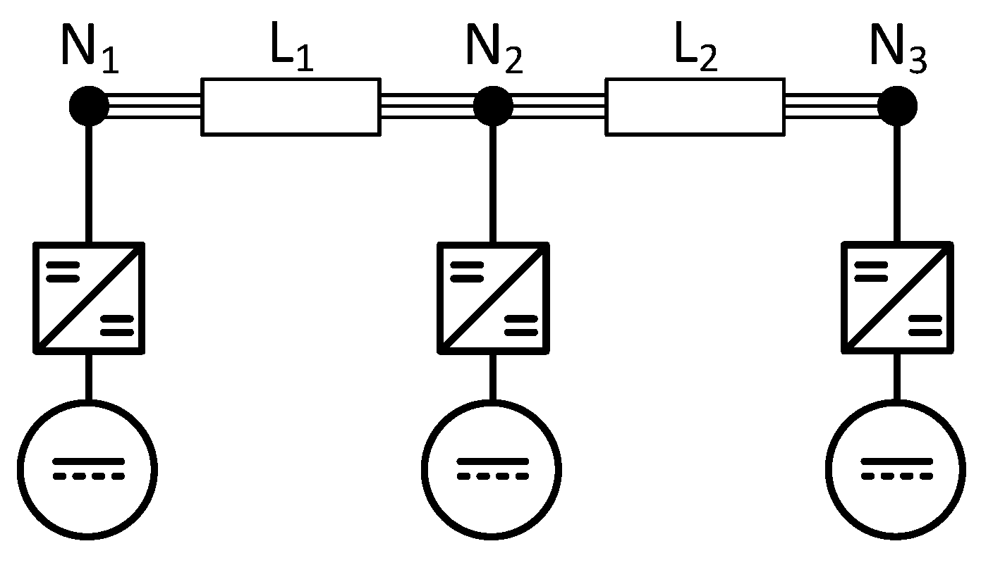
5.1. Bus Configuration

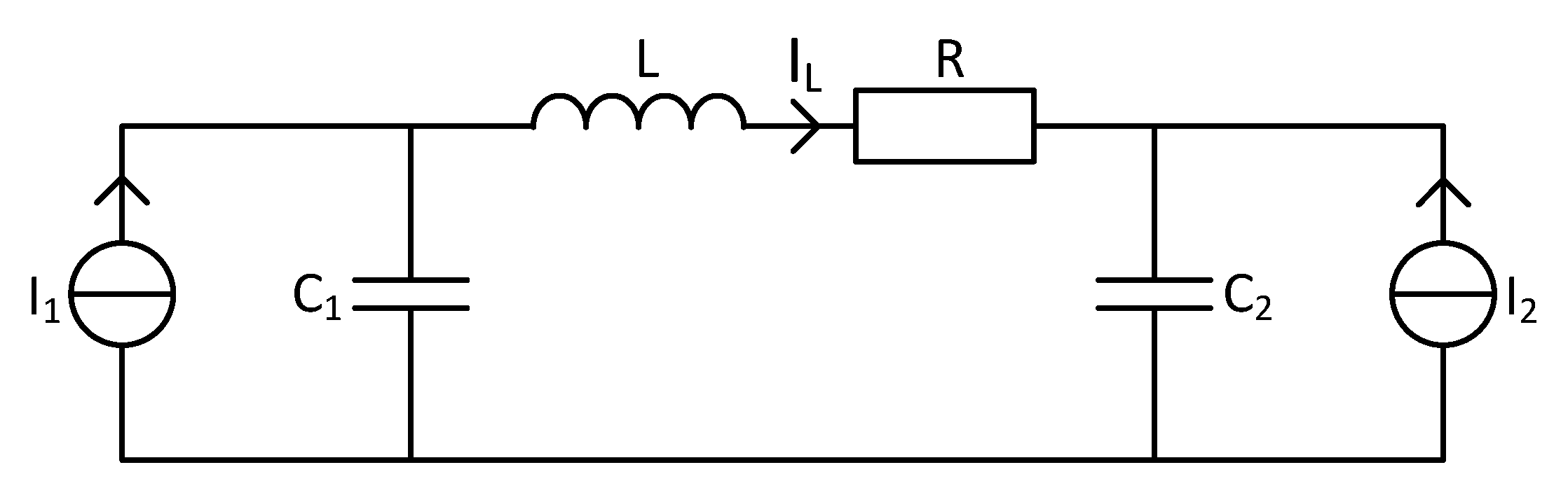
An example of a DC distribution system in a bus configuration is shown in Figure 5. The idea of such a configuration is one “bus”, or set of distribution lines, without branches or meshes. For the shown example, it is assumed that a source is situated at $N_1$ and a load is situated at both $N_2$ and $N_3$. However, the derivation for other configurations is analogous. For the sake of simplicity, the resistance of the distribution lines is neglected.

Using Equations (30) and (33), the coefficients of the characteristic equation are derived to be

$$\begin{array}{cc}\hfill a_1& =1,\hfill \end{array}$$

(44)

$$\begin{array}{cc}\hfill a_2& =\frac{1}{C_1{Z}_1}+\frac{1}{C_2{Z}_2}+\frac{1}{C_3{Z}_3},\hfill \end{array}$$

(45)

$$\begin{array}{ll}{a}_3=& \frac{1}{C_1{L}_1}+\frac{1}{C_2{L}_1}+\frac{1}{C_2{L}_2}+\frac{1}{C_3{L}_2}+\\ & \frac{1}{C_1{Z}_1{C}_2{Z}_2}+\frac{1}{C_1{Z}_1{C}_3{Z}_3}+\frac{1}{C_2{Z}_2{C}_3{Z}_3},\end{array}$$

(46)

$$\begin{array}{ll}{a}_4=& \frac{1}{C_1{Z}_1{C}_2{Z}_2{C}_3{Z}_3}+\frac{1}{C_1{L}_1{C}_2{Z}_2}+\frac{1}{C_1{L}_1{C}_3{Z}_3}+\\ & \frac{1}{C_2{L}_1{C}_3{Z}_3}+\frac{1}{C_2{L}_1{C}_1{Z}_1}+\frac{1}{C_2{L}_2{C}_1{Z}_1}+\\ & \frac{1}{C_2{L}_2{C}_3{Z}_3}+\frac{1}{C_3{L}_2{C}_2{Z}_2}+\frac{1}{C_3{L}_2{C}_1{Z}_1},\end{array}$$

(47)

$$\begin{array}{ll}{a}_5=& \frac{1}{C_1{Z}_1{C}_2{Z}_2{C}_3{L}_2}+\frac{1}{C_1{Z}_1{C}_3{Z}_3{C}_2{L}_1}+\\ & \frac{1}{C_1{Z}_1{C}_3{Z}_3{C}_2{L}_2}+\frac{1}{C_2{Z}_2{C}_3{Z}_3{C}_1{L}_1}+\\ & \frac{1}{C_1{L}_1{C}_2{L}_2}+\frac{1}{C_1{L}_1{C}_3{L}_2}+\frac{1}{C_2{L}_1{C}_3{L}_2},\end{array}$$

(48)

$$\begin{array}{ll}{a}_6=& \frac{1}{C_1{Z}_1{C}_2{L}_1{C}_3{L}_2}+\frac{1}{C_2{Z}_2{C}_1{L}_1{C}_3{L}_2}+\\ & \frac{1}{C_3{Z}_3{C}_1{L}_1{C}_2{L}_2}.\end{array}$$

(49)

Now if, for simplicity, we assume that the capacitance in each node ($C_i$) and inductance in each distribution line ($L_j$) are equal, we arrive at two simple requirements for the stability of this system

$$\begin{array}{cc}\hfill Z_1& <\frac{-1}{\frac{1}{Z_2}+\frac{1}{Z_3}},\hfill \end{array}$$

(50)

$$\begin{array}{cc}\hfill Z_1& >\frac{-2Z_2-Z_3}{1+\frac{3C{Z}_2{Z}_3}{L}},\hfill \end{array}$$

(51)

where the first requirement is derived from the even coefficients, and the second requirement follows from the odd coefficients. Interestingly, from these requirements, a constraint on the capacitance and inductance follows:

$$\frac{3C}{L}>\frac{2}{Z_3^2}+\frac{1}{Z_2^2}+\frac{2}{Z_2{Z}_3},$$

(52)

which defines a minimum on the ratio between the capacitance and inductance for feasible stability.

The derived requirements are necessary but not sufficient for stability. To make the set of requirements sufficient additional constraints can be derived from the Routh coefficients. In general, the requirements derived from the Routh coefficients are more complex, but similar to the requirements derived from the characteristic equation’s coefficients (see (23)). For this example, according to Equations (40) and (41), if the ratio between the capacitance and inductance is large enough, it is sufficient if

$$\begin{array}{cc}\hfill Z_1& <\frac{-1}{\frac{1}{Z_2}+\frac{4}{Z_3}},\hfill \end{array}$$

(53)

which, agreeably, is a stricter version of Equation (50) derived from the characteristic equation’s coefficients.

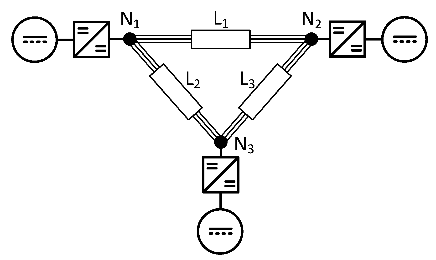
5.2. Ring Configuration

The second example is a DC distribution system in a “ring” configuration shown in Figure 6. In this case, the ring configuration does not have any branches, but it is meshed. In this example, the source is located at $N_1$ and loads are located at $N_2$ and $N_3$.

Analogous to the bus configuration, the requirements for stability of this system can be derived from the characteristic equation. These requirements are derived to be

$$\frac{-Z_2-Z_3}{1+\frac{9C{Z}_2{Z}_3}{2L}}<Z_1<\frac{-1}{\frac{1}{Z_2}+\frac{1}{Z_3}}.$$

(54)

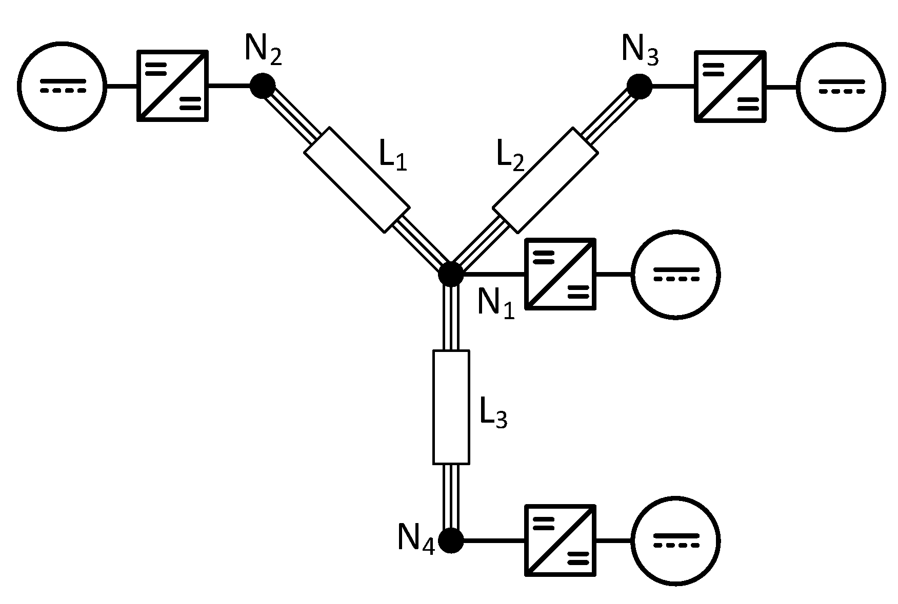
5.3. Star Configuration

The last example is a DC distribution system in a “star” configuration, which is shown in Figure 7. In this case, the star configuration has branches, but no meshes. Since, in most cases, the source is situated in the center node, and it is assumed that the system has a source placed at $N_1$ and a load is placed at $N_2$, $N_3$ and $N_4$.

Analogous to the previous configurations, the requirements for stability of this system are derived to be

$$\frac{\frac{1}{2}(-Z_2{Z}_3-Z_2{Z}_4-Z_3{Z}_4)}{Z_2+Z_3+Z_4+\frac{2C{Z}_2{Z}_3{Z}_4}{L}}<Z_1<\frac{-3}{\frac{5}{Z_2}+\frac{5}{Z_3}+\frac{5}{Z_4}}.$$

(55)

The stability requirements for the three examples show strong congruence with respect to the sensitivity towards, for example, inductance and capacitance. Therefore, it becomes viable to make some general conclusions.

5.4. Sensitivity Analysis

Similar results with respect to previous work are found for some parameters. With respect to inductance, the results of this paper are congruent with previous works [26,37], where a decrease in inductance leads to increased stability. Furthermore, from the equations in the previous section, it can be observed that the impedance (slope) of the droop controlled source has an upper and lower bound. The upper bound is related to the constant power loads in the system, while the lower bound is related to the oscillations in the system. These oscillations originate from the interaction of capacitance at different nodes through the lines’ inductance. These results are also congruent with previous work [43,44].

Generally, it is thought that an increase in capacitance is beneficial for the stability of the system. From Equations (52), (54) and (55), it is clear that there is a minimum required capacitance and further increase of capacitance leads to an increased stability margin. However, Equations (45) and (49) suggest a negative effect on the overall damping of the system. The second ($a_2$) and last ($a_{N+L}$) coefficients are the sum and product of all eigenvalues, respectively. Therefore, when the capacitance is increased the sum and product of all eigenvalues are decreased leading to decreased damping in the system. Conceptually, this can also be understood, a voltage deviation with larger capacitance means a larger disparity in energy, which will take a long(er) time to be damped.

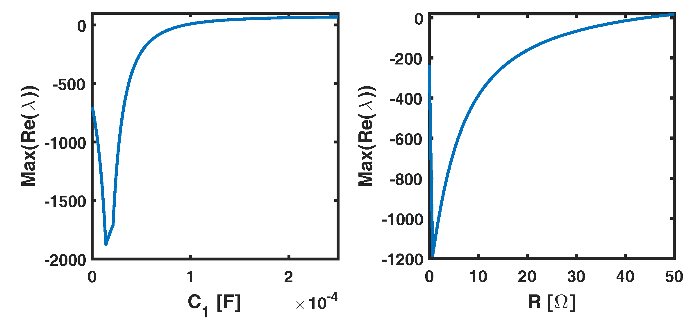
Interestingly, Equations (45) and (49) suggest that decreasing the source capacitance compared to the load capacitance has a positive influence on the damping in the system. However, this not necessarily infinitely valid since the decrease of source impedance also has a negative effect on some of the coefficients (e.g., $a_3$). As validation of this observation, the maximum real part of the eigenvalues as function of the source capacitance is shown in Figure 8, in which it can be seen that a reduction of the source capacitance leads to increased stability, but only up until a certain capacitance. The parameters used for both numerical calculations, unless otherwise specified, are given in

Table 1. System parameters for the sensitivity analysis.

$\mathit{R}\left[\mathsf{\Omega }\right]$	L [mH]	C [$\mathsf{\mu }$F]	${\mathit{Z}}_1\left[\mathsf{\Omega }\right]$	${\mathit{Z}}_2\left[\mathsf{\Omega }\right]$
0	$0.36$	50	5	$-125$

.

Moreover, since the effect of the resistance has been excluded from the mathematical derivations (for the sake of simplicity), another numerical calculation was performed to show the effect of resistance on the damping in the system. Figure 8 shows that some resistance is beneficial for the stability, while larger values deteriorate stability. The positive effect can be explained by the additional damping in the system while the negative effect on stability stems from the current limiting characteristic of the resistance.

6. Simulation Results

In this section, two simulations are performed for all three example systems to illustrate the results of the previous sections. Firstly, the configurations are simulated with a too high droop impedance to illustrate one of the unstable conditions of DC distribution systems. Secondly, the configurations are simulated with an acceptable droop impedance to illustrate the behavior of stable DC distribution systems and to compare it to the previous simulations.

For the simulations the example configurations, shown in Figure 5, Figure 6 and Figure 7, are used. For each configuration, the source is situated at node $N_1$, while loads are situated at $N_2$, $N_3$ and $N_4$. The system parameters, which are used for all simulations, are given in

Table 2. System parameters for the stability simulations.

${\mathit{R}}_{\mathit{l}}\left[\mathsf{\Omega }\right]$	${\mathit{L}}_{\mathit{l}}$ [mH]	${\mathit{C}}_{\mathit{l}}$ [$\mathsf{\mu }$F]	${\mathit{C}}_{\mathit{c}}$ [$\mathsf{\mu }$F]
$4.61$	$0.36$	$0.172$	5.0

. In the table, $R_l$, $L_l$ and $C_l$ are the resistance, inductance and capacitance of the distribution lines, respectively. Furthermore, $C_c$ is the (grid-side) output capacitance of the source and load converters.

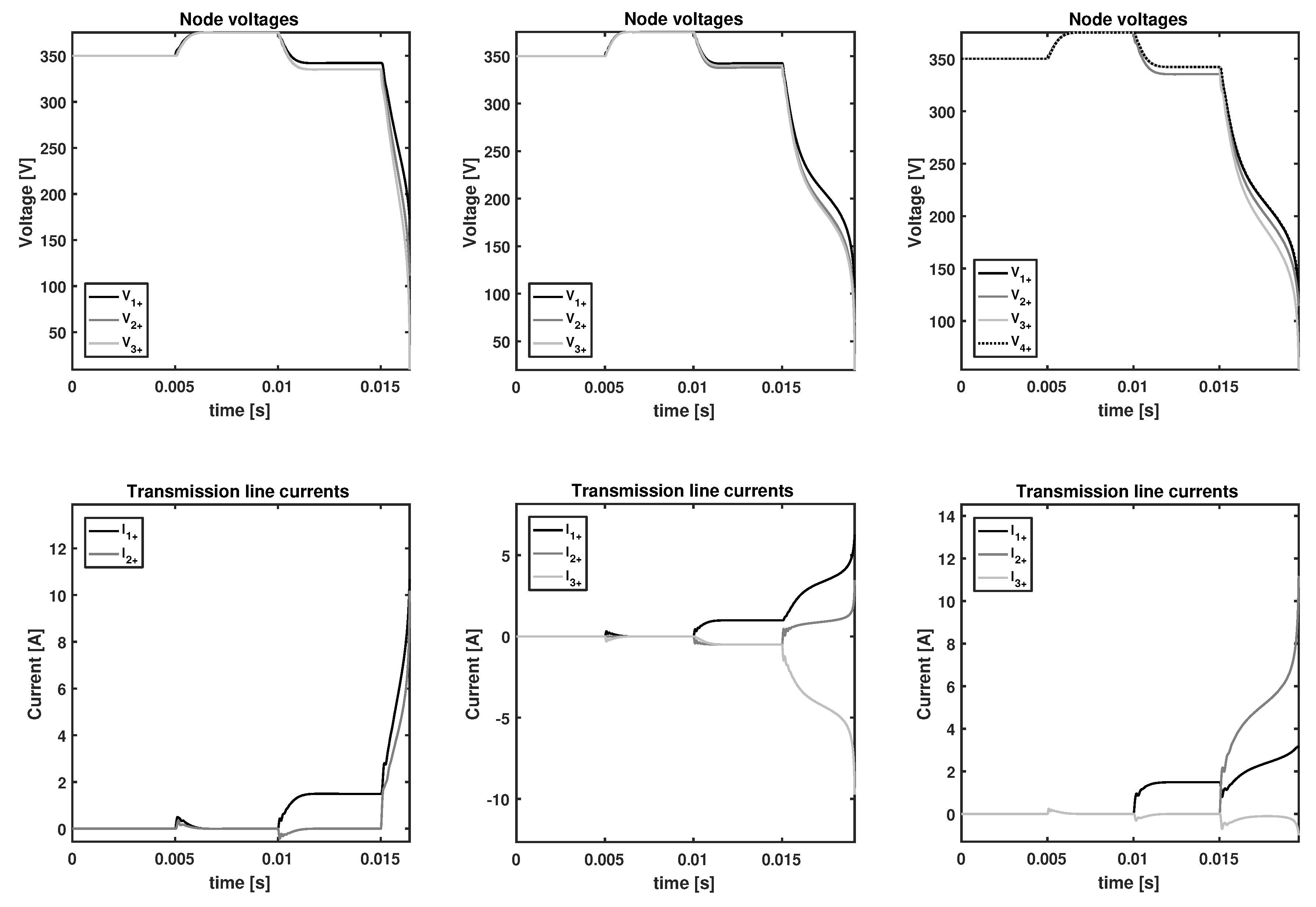
For the first set of simulations, the source reference voltage is initially set at $350$V with a droop impedance of $22\mathsf{\Omega }$. At $t=5$ms, the reference voltage of the source is changed to $375$V. Subsequently, at $t=10$ms a (constant power) load of $500$W is switched on at $N_2$. Lastly, at $t=15$ms, a load of $1000$W is switched on at $N_3$.

The results of these simulations are shown in Figure 9. It is seen that the system reacts stably to changes in load and voltage reference until the total load exceeds the stability conditions. Consequently, after $t=15$ms, the current rises exponentially over time and the voltage falls to zero.

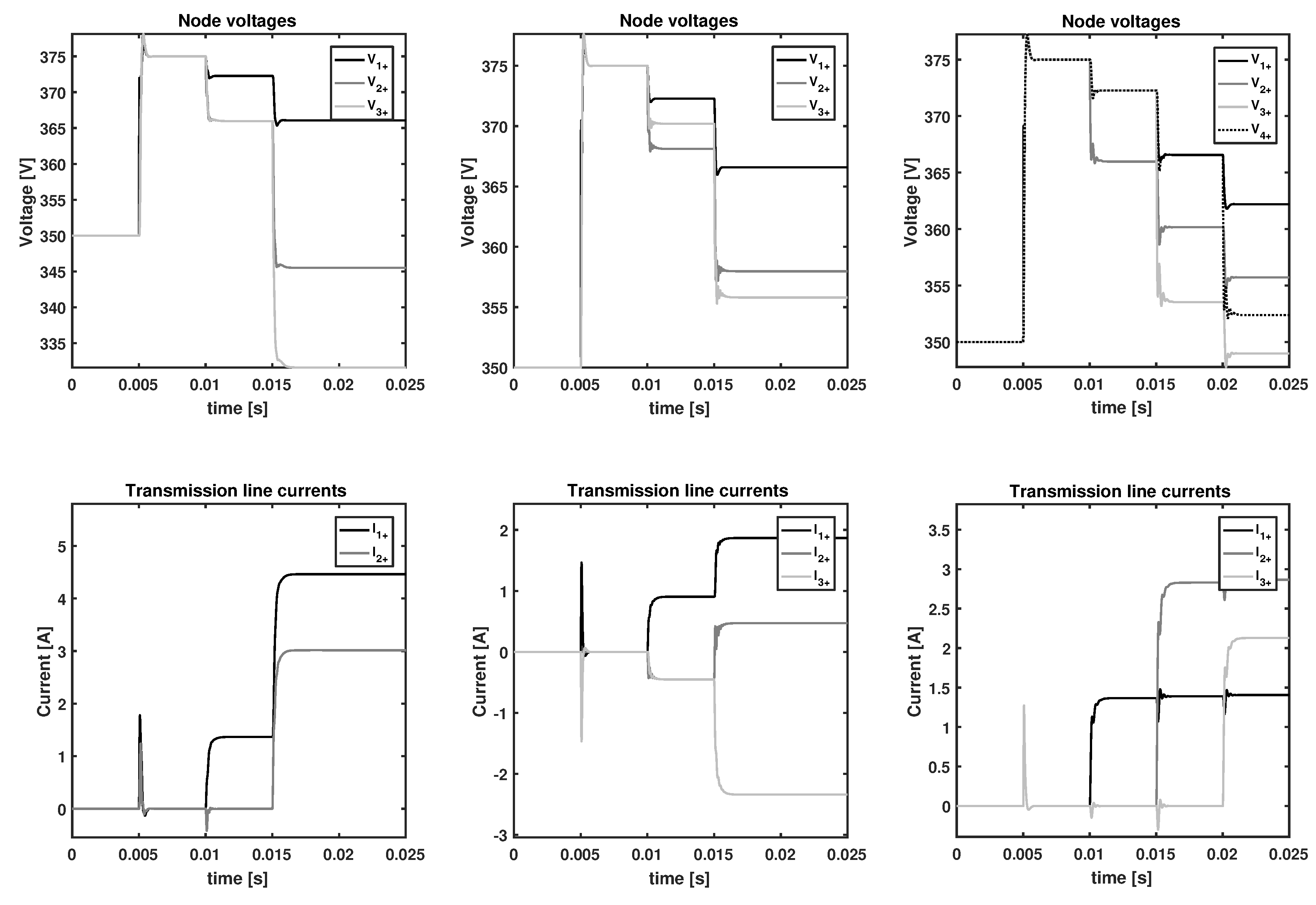
For the second simulations, the source reference voltage is initially set at $350$V with a droop impedance of $2\mathsf{\Omega }$. At $t=5$ms, the reference voltage of the source is changed to $375$V. Afterwards, at $t=10,15,20$ms loads of 500, 1000 and $750$W are switched on at $N_2$, $N_3$ and $N_4$, respectively.

The results of these simulations are shown in Figure 10. Firstly, it is seen that the voltage deviation from the reference voltage is lower compared to the previous simulations. Secondly, due to the lower droop impedance, the systems achieve their steady state faster than in the previous simulations (but this also causes some oscillations). Lastly, the systems are stable as the oscillations damp out and the voltages remain stably at their operating point.

In Figure 9, it was seen that instability occurs when the source impedance is too high. In this case, there does not exist a steady state voltage as a result of the interaction between the droop controlled source and the constant power load. Furthermore, the systems reach a state where they are no longer stable (and have eigenvalue(s) with a positive real part).

Figure 10 shows that, since the droop controlled source has a low impedance, the system reaches a steady state faster. The second simulations also show oscillations, which are caused by the stronger reaction of the source to a deviation in voltage. These oscillations originate from the interaction between the capacitance of the nodes through the inductance of the distribution lines. If the source impedance and line resistance are too low, these oscillations might not be sufficiently damped out and a different type of instability can occur. In this case, the steady state voltage might exist, but oscillations around this steady state voltage increase or are not damped (enough). Conceptually, this can also be explained. If the impedance of the droop-controlled source is small, it will approximately behave as a constant voltage source. Consequently, the source will provide no damping in the system at all (see the first example in Section 3). In other words, for DC distribution systems to be called (sufficiently) stable, there should exist a stable steady state and there should be enough damping on the oscillations in the system.

7. Conclusions

This paper introduced a state-space model that represents any DC distribution system by its nodes, distribution lines, and source and load converters. The model allows for straightforward formulation of the state-space matrices, which relies on the validity of averaging, linearization and simplification of the electronic power converters.

The stability of DC distribution systems is derived from the eigenvalues of their state-space matrices. The stability of two simple examples was derived to illustrate the approach. Furthermore, a generalized method was presented to algebraically analyze the stability of any DC distribution system. To guarantee that the eigenvalues have only negative real parts, and thus guarantee stability, a method to derive the necessary and sufficient conditions was presented.

Subsequently, three examples were used to demonstrate how the presented method can lead to requirements for the stability of DC distribution systems. The three example systems showed strong congruency with respect to their sensitivity towards, for example, inductance and capacitance. Moreover, a sensitivity analysis was performed to verify the relationship between the inductance, droop source impedance, capacitance and resistance to the stability (and damping) of a system. The results showed that increasing inductance has a negative effect on stability, that increasing load capacitance has a positive effect, and that the droop impedance has a upper and lower limit (in agreement with previous research). However, it was also shown that both large and small values of the resistance and source capacitance have a negative effect on the stability of the system. This algebraically appends and verifies conclusions on parameter sensitivity of previous research for a large variety of DC distribution systems.

Additionally, various simulations were performed to show the dynamic behavior of a DC distribution system under stable and unstable conditions. These simulations showed two main modes of instability. Firstly, when the droop controlled sources’ impedance is too large. In this case, the constant power loads’ current increases as the voltage drops, and, as a result, the voltage of the entire system drops to 0 V. Secondly, if there is not enough damping from the source (and distribution lines’ resistance). In the latter case, the insufficient damping results in increasing oscillations (which originate from the interactions between the different node capacitance).

In the future, the developed method could be used to evaluate and improve the stability of DC distribution systems. Furthermore, it could be used by the control system to, for example, assess if loads are allowed to turn on, if loads should switch off, or to change the control settings of sources.

References

- Flourentzou, N.; Agelidis, V.G.; Demetriades, G.D. VSC-Based HVDC Power Transmission Systems: An Overview. IEEE Trans. Power Electron. 2009, 24, 592–602. [Google Scholar] [CrossRef]
- Ghareeb, A.T.; Mohamed, A.A.; Mohammed, O.A. DC microgrids and distribution systems: An overview. In Proceedings of the 2013 IEEE Power Energy Society General Meeting, Vancouver, BC, Canada, 21–25 July 2013; pp. 1–5. [Google Scholar]
- Becker, D.J.; Sonnenberg, B.J. DC microgrids in buildings and data centers. In Proceedings of the 2011 IEEE 33rd International Telecommunications Energy Conference (INTELEC), Amsterdam, The Netherlands, 9–13 October 2011; pp. 1–7. [Google Scholar]
- Pratt, A.; Kumar, P.; Aldridge, T.V. Evaluation of 400V DC distribution in telco and data centers to improve energy efficiency. In Proceedings of the INTELEC 07—29th International Telecommunications Energy Conference, Rome, Italy, 30 September–4 October 2007; pp. 32–39. [Google Scholar]
- Thomas, B.A.; Azevedo, I.L.; Morgan, G. Edison Revisited: Should we use DC circuits for lighting in commercial buildings? Energy Policy 2012, 45, 399–411. [Google Scholar] [CrossRef]
- Wunder, B.; Ott, L.; Szpek, M.; Boeke, U.; Weiß, R. Energy efficient DC-grids for commercial buildings. In Proceedings of the 2014 IEEE 36th International Telecommunications Energy Conference (INTELEC), Vancouver, BC, Canada, 28 September–2 October 2014; pp. 1–8. [Google Scholar]
- Rodriguez-Diaz, E.; Savaghebi, M.; Vasquez, J.C.; Guerrero, J.M. An overview of low voltage DC distribution systems for residential applications. In Proceedings of the 2015 IEEE 5th International Conference on Consumer Electronics—Berlin (ICCE-Berlin), Berlin, Germany, 6–9 September 2015; pp. 318–322. [Google Scholar]
- Patterson, B.T. DC, Come Home: DC Microgrids and the Birth of the “Enernet”. IEEE Power Energy Mag. 2012, 10, 60–69. [Google Scholar] [CrossRef]
- Vossos, V.; Garbesi, K.; Shen, H. Energy savings from direct-DC in U.S. residential buildings. Energy Build. 2014, 68 Pt A, 223–231. [Google Scholar] [CrossRef]
- Costa, M.A.D.; Costa, G.H.; dos Santos, A.S.; Schuch, L.; Pinheiro, J.R. A high efficiency autonomous street lighting system based on solar energy and LEDs. In Proceedings of the 2009 Brazilian Power Electronics Conference, Bonito-Mato Grosso do Sul, Brazil, 27 September–1 October 2009; pp. 265–273. [Google Scholar]
- Hulsebosch, M.; Willigenburg, P.; Woudstra, J.; Groenewald, B. Direct current in public lighting for improvement in LED performance and costs. In Proceedings of the 2014 International Conference on the Eleventh Industrial and Commercial Use of Energy, Cape Town, South Africa, 19–20 August 2014; pp. 1–9. [Google Scholar]
- Planas, E.; Andreu, J.; Garate, J.I.; de Alegria, I.M.; Ibarra, E. AC and DC technology in microgrids: A review. Renew. Sustain. Energy Rev. 2015, 43, 726–749. [Google Scholar] [CrossRef]
- Mackay, L.; Hailu, T.G.; Mouli, G.C.; Ramirez-Elizondo, L.; Ferreira, J.A.; Bauer, P. From DC nano- and microgrids towards the universal DC distribution system—A plea to think further into the future. In Proceedings of the 2015 IEEE Power Energy Society General Meeting, Denver, CO, USA, 26–30 July 2015; pp. 1–5. [Google Scholar]
- Driesen, J.; Visscher, K. Virtual synchronous generators. In Proceedings of the 2008 IEEE Power and Energy Society General Meeting—Conversion and Delivery of Electrical Energy in the 21st Century, Pittsburgh, PA, USA, 20–24 July 2008; pp. 1–3. [Google Scholar]
- Bottrell, N.; Prodanovic, M.; Green, T.C. Dynamic Stability of a Microgrid With an Active Load. IEEE Trans. Power Electron. 2013, 28, 5107–5119. [Google Scholar] [CrossRef]
- Cespedes, M.; Xing, L.; Sun, J. Constant-Power Load System Stabilization by Passive Damping. IEEE Trans. Power Electron. 2011, 26, 1832–1836. [Google Scholar] [CrossRef]
- Cespedes, M.; Beechner, T.; Xing, L.; Sun, J. Stabilization of constant-power loads by passive impedance damping. In Proceedings of the 2010 Twenty-Fifth Annual IEEE Applied Power Electronics Conference and Exposition (APEC), Palm Springs, CA, USA, 21–25 February 2010; pp. 2174–2180. [Google Scholar]
- Dragicevic, T.; Lu, X.; Vasquez, J.C.; Guerrero, J.M. DC Microgrids—Part I: A Review of Control Strategies and Stabilization Techniques. IEEE Trans. Power Electron. 2016, 31, 4876–4891. [Google Scholar] [CrossRef]
- Kwasinski, A.; Onwuchekwa, C.N. Dynamic Behavior and Stabilization of DC Microgrids With Instantaneous Constant-Power Loads. IEEE Trans. Power Electron. 2011, 26, 822–834. [Google Scholar] [CrossRef]
- Ahmadi, R.; Ferdowsi, M. Improving the Performance of a Line Regulating Converter in a Converter-Dominated DC Microgrid System. IEEE Trans. Smart Grid 2014, 5, 2553–2563. [Google Scholar] [CrossRef]
- Riccobono, A.; Santi, E. Comprehensive Review of Stability Criteria for DC Power Distribution Systems. IEEE Trans. Ind. Appl. 2014, 50, 3525–3535. [Google Scholar] [CrossRef]
- Wang, X.; Yao, R.; Rao, F. Three-step impedance criterion for small-signal stability analysis in two-stage DC distributed power systems. IEEE Power Electron. Lett. 2003, 1, 83–87. [Google Scholar] [CrossRef]
- Zadeh, M.K.; Gavagsaz-Ghoachani, R.; Martin, J.P.; Pierfederici, S.; Nahid-Mobarakeh, B.; Molinas, M. Discrete-time modelling, stability analysis, and active stabilization of DC distribution systems with constant power loads. In Proceedings of the 2015 IEEE Applied Power Electronics Conference and Exposition (APEC), Charlotte, NC, USA, 15–19 March 2015; pp. 323–329. [Google Scholar]
- Sulligoi, G.; Bosich, D.; Giadrossi, G.; Zhu, L.; Cupelli, M.; Monti, A. Multiconverter Medium Voltage DC Power Systems on Ships: Constant-Power Loads Instability Solution Using Linearization via State Feedback Control. IEEE Trans. Smart Grid 2014, 5, 2543–2552. [Google Scholar] [CrossRef]
- Sanchez, S.; Molinas, M. Degree of Influence of System States Transition on the Stability of a DC Microgrid. IEEE Trans. Smart Grid 2014, 5, 2535–2542. [Google Scholar] [CrossRef]
- Hailu, T.; Mackay, L.; Ramirez-Elizondo, L.; Gu, J.; Ferreira, J.A. Voltage weak DC microgrid. In Proceedings of the 2015 IEEE First International Conference on DC Microgrids (ICDCM), Atlanta, GA, USA, 7–10 June 2015; pp. 138–143. [Google Scholar]
- Lu, X.; Sun, K.; Huang, L.; Guerrero, J.M.; Vasquez, J.C.; Xing, Y. Virtual impedance based stability improvement for DC microgrids with constant power loads. In Proceedings of the 2014 IEEE Energy Conversion Congress and Exposition (ECCE), Pittsburgh, PA, USA, 14–18 September 2014; pp. 2670–2675. [Google Scholar]
- Makrygiorgou, D.I.; Alexandridis, A.T. Stability Analysis of DC Distribution Systems with Droop-Based Charge Sharing on Energy Storage Devices. Energies 2017, 10, 433. [Google Scholar] [CrossRef]
- Makrygiorgou, D.I.; Alexandridis, A.T. Modeling and stability of autonomous DC microgrids with converter-controlled energy storage systems. In Proceedings of the 2017 IEEE Second International Conference on DC Microgrids (ICDCM), Nuremburg, Germany, 27–29 June 2017; pp. 285–291. [Google Scholar]
- Bosich, D.; Gibescu, M.; Sulligoi, G. Large-signal stability analysis of two power converters solutions for DC shipboard microgrid. In Proceedings of the 2017 IEEE Second International Conference on DC Microgrids (ICDCM), Nuremburg, Germany, 27–29 June 2017; pp. 125–132. [Google Scholar]
- Belk, J.A.; Inam, W.; Perreault, D.J.; Turitsyn, K. Stability and Control of Ad Hoc DC Microgrids. Proceedings of Decision and Control (CDC), 2016 IEEE 55th Conference on, Las Vegas, NV, USA, 12–14 December 2016. [Google Scholar]
- van der Blij, N.H.; Ramirez-Elizondo, L.M.; Bauer, P.; Spaan, M.T.J. Design guidelines for stable DC distribution systems. In Proceedings of the 2017 IEEE Second International Conference on DC Microgrids (ICDCM), Nuremburg, Germany, 27–29 June 2017; pp. 279–284. [Google Scholar]
- Abdelwahed, M.A.; El-Saadany, E.F. Droop gains selection methodology for offshore multi-terminal HVDC networks. In Proceedings of the 2016 IEEE Electrical Power and Energy Conference (EPEC), Ottawa, ON, Canada, 12–14 October 2016; pp. 1–5. [Google Scholar]
- Shamsi, P.; Fahimi, B. Stability Assessment of a DC Distribution Network in a Hybrid Micro-Grid Application. IEEE Trans. Smart Grid 2014, 5, 2527–2534. [Google Scholar] [CrossRef]
- Tabari, M.; Yazdani, A. A Mathematical Model for Stability Analysis of a DC Distribution System for Power System Integration of Plug-In Electric Vehicles. IEEE Trans. Veh. Technol. 2015, 64, 1729–1738. [Google Scholar] [CrossRef]
- Jin, Z.; Meng, L.; Guerrero, J.M. Comparative admittance-based analysis for different droop control approaches in DC microgrids. In Proceedings of the 2017 IEEE Second International Conference on DC Microgrids (ICDCM), Nuremburg, Germany, 27–29 June 2017; pp. 515–522. [Google Scholar]
- Anand, S.; Fernandes, B.G. Reduced-Order Model and Stability Analysis of Low-Voltage DC Microgrid. IEEE Trans. Ind. Electron. 2013, 60, 5040–5049. [Google Scholar] [CrossRef]
- Van der Blij, N.H.; Ramirez-Elizondo, L.M.; Spaan, M.T.J.; Bauer, P. A State-Space Approach to Modelling DC Distribution Systems. IEEE Trans. Power Syst. 2017, PP, 1. [Google Scholar] [CrossRef]
- Zadeh, L.; Desoer, C. Linear System Theory: The State Space Approach; McGraw-Hill Series in System Science; McGraw-Hill: New York, NY, USA, 1963. [Google Scholar]
- Mirsky, L. An Introduction to Linear Algebra; Dover Books on Mathematics; Dover Publications: New York, NY, USA, 2012. [Google Scholar]
- Seroul, R. Programming for Mathematicians; Universitext; Springer: Berlin/Heidelberg, Germany, 2000. [Google Scholar]
- Barnett, S.; Šiljak, D. Routh’s algorithm: A centennial survey. SIAM Rev. 1977, 19, 472–489. [Google Scholar] [CrossRef]
- Gao, F.; Bozhko, S.; Costabeber, A.; Patel, C.; Wheeler, P.; Hill, C.I.; Asher, G. Comparative Stability Analysis of Droop Control Approaches in Voltage-Source-Converter-Based DC Microgrids. IEEE Trans. Power Electron. 2017, 32, 2395–2415. [Google Scholar] [CrossRef]
- Korompili, A.; Monti, A. Analysis of the dynamics of dc voltage droop controller of dc-dc converters in multi-terminal dc grids. In Proceedings of the 2017 IEEE Second International Conference on DC Microgrids (ICDCM), Nuremburg, Germany, 27–29 June 2017; pp. 507–514. [Google Scholar]
Figure 1.
Bipolar DC distribution system containing storage, sources and loads.
Figure 2.
Equivalent circuits of droop controlled sources (left) and constant power loads (right).
Figure 3.
Simple DC distribution grid containing a constant power load and a voltage source connected via a distribution line.
Figure 4.
Simple DC distribution grid containing a constant power load and a droop controlled source connected via a distribution line.
Figure 5.
Example of a DC distribution grid with three nodes and two lines in a bus configuration.
Figure 6.
Example of a DC distribution grid with three nodes and three lines in a ring configuration.
Figure 7.
Example of a DC distribution grid with four nodes and three lines in a star configuration.
Figure 8.
Maximum real part of the eigenvalues of as function of the source capacitance (left) and the line resistance (right) for the bus example.
Figure 9.
Node voltages and distribution line currents of the bus (left), ring (middle) and star (right) example systems under changing loads and reference voltages, with a droop impedance of 22 .
Figure 10.
Node voltages and distribution line currents of the bus (left), ring (middle) and star (right) example systems under changing loads and reference voltages, with a droop impedance of 2 .