Design and Numerical Simulations of a Flow Induced Vibration Energy Converter for Underwater Mooring Platforms

1
School of Marine Science and Technology, Northwestern Polytechnical University, Xi’an 710072, China
2
Key Laboratory for Unmanned Underwater Vehicle, Northwestern Polytechnical University, Xi’an 710072, China
*
Author to whom correspondence should be addressed.
Energies 2017, 10(9), 1427; https://doi.org/10.3390/en10091427
Submission received: 14 July 2017
/
Revised: 10 September 2017
/
Accepted: 14 September 2017
/
Published: 16 September 2017
(This article belongs to the Section F: Electrical Engineering)
Abstract
:Limited battery energy restricts the duration of the underwater operation of underwater mooring platforms (UMPs). In this paper, a flow-induced vibration energy converter (FIVEC) is designed to produce power for the UMPs and extend their operational time. The FIVEC is equipped with a thin plate to capture the kinetic energy in the vortices shed from the surface of the UMP. A magnetic coupling (MC) is applied for the non-contacting transmission of the plate torque to the generators so that the friction loss can be minimized. In order to quantify and evaluate the performance of the FIVEC, two-dimensional computational fluid dynamics (CFD) simulations are performed. Simulations are based on the Reynolds Averaged Navier-Stokes (RANS) equations and the shear stress transport (SST) k-ω turbulent model is utilized. The CFD method is firstly validated using existing experimental data. Then the influences of plate length and system damping on the performance of the FIVEC are evaluated. The results show that the device has a maximum averaged power coefficient of 0.0520 (13.86 W) in the considered situations. The results also demonstrate the feasibility of this energy converter plan.
1. Introduction
Underwater mooring platforms (UMPs) are a class of underwater devices which are tethered to the seabed using mooring cables. UMPs have broad applications in both civil and military missions, such as underwater monitoring (oceanographic sensors), communication (acoustic communication nodes), and defense (mooring mines), with expected performance durations typically ranging from months to years. Nowadays increasing emphasis has been put on the improvement of UMPs. The greatest concern for the UMPs is the duration of their underwater operation, which is mainly determined by the total energy contained in the on-board batteries and the uninterrupted consumption of energy by the electronic devices. Although most UMPs are designed with low-power configurations now, the operation durations are still not satisfying due to the limited battery energy. Extending the operational life of UMPs can significantly reduce the cost for missions where a sustained presence is required, because of the high costs associated with retrieving, repowering, and redeploying remote systems.
UMPs stay in the ocean environment once deployed. The ocean has proved to be a promising source of renewable energies, including ocean surface solar energy [1], wave energy [2,3], current energy [4], thermal energy [5], and osmotic energy [6]. If these types of energy can be extracted to recharge the batteries of the UMPs, the underwater operation duration can be greatly extended. Although some of the above types of energy have been studied to power ocean devices, such as solar-powered autonomous underwater vehicles (AUVs) [7], solar-powered ships [8], and thermal-powered underwater gliders [9,10], they are not suitable for powering UMPs. UMPs are usually moored tens to hundreds of meters beneath the ocean surface, where solar energy and wave energy attenuate quickly and could hardly be utilized. As for the thermal energy, the UMPs, which are expected to perform fixed-point monitoring, cannot move vertically to pass through a thermocline to gain the thermal energy like the underwater gliders [10].
UMPs are often deployed where ocean currents are consistently available. The kinetic energy stored in ocean currents provides an ideal energy source to recharge the UMPs. In previous studies, specially-designed ocean current turbines (OCTs) have been proposed for UMPs to generate electricity from the currents [11,12]. The use of the OCTs could extend the operation life of the UMPs, however, the OCTs have complex structures and show poor feasibility [12]. Additionally, the OCT applies extra thrust and torque on the mooring system when rotating, making it harder for the UMP to reach motion stability [13].
The flow-induced motion (FIM) conversion technology provides another way to utilize the ocean current energy. It is known that flow passing blunt bodies experiences unsteady separation and forms a wake of repeating swirling vortices, known as the Karman vortex street. The FIM generates kinetic energy from the surface-shed vortices and converts the kinetic energy into electricity. The FIM can be roughly divided into two groups, vortex-induced vibration (VIV) and galloping [14]. VIV is caused by periodically-shed vortices which generate an asymmetric pressure distribution around the body and provide periodic forces that lead to a vibration in the body. Galloping is known as a dynamic instability that is induced in an elastic structure due to internal turbulence of the fluid or any reason which provides initial disturbance. A detailed review of the FIM devices can be found in [15]. The idea of the VIV is first proposed by Bernitsas and Raghavan [16], and further developed by the Marine Renewable Energy Laboratory at the University of Michigan [17,18,19]. They built an energy converter named VIVACE (Vortex-Induced Vibration Aquatic Clean Energy) that uses a passive circular cylinder with upward-downward motion induced by vortex shedding. Over the past few years, comprehensive research has been done to reveal the mechanism of the flow-structure interaction and to enhance the power efficiency of the VIV device, including the influences of the cross-sections [20], the spring stiffness [21], damping ratio [22], mass ratio [23], passive turbulence control structure [24], and multiple cylinders [25].
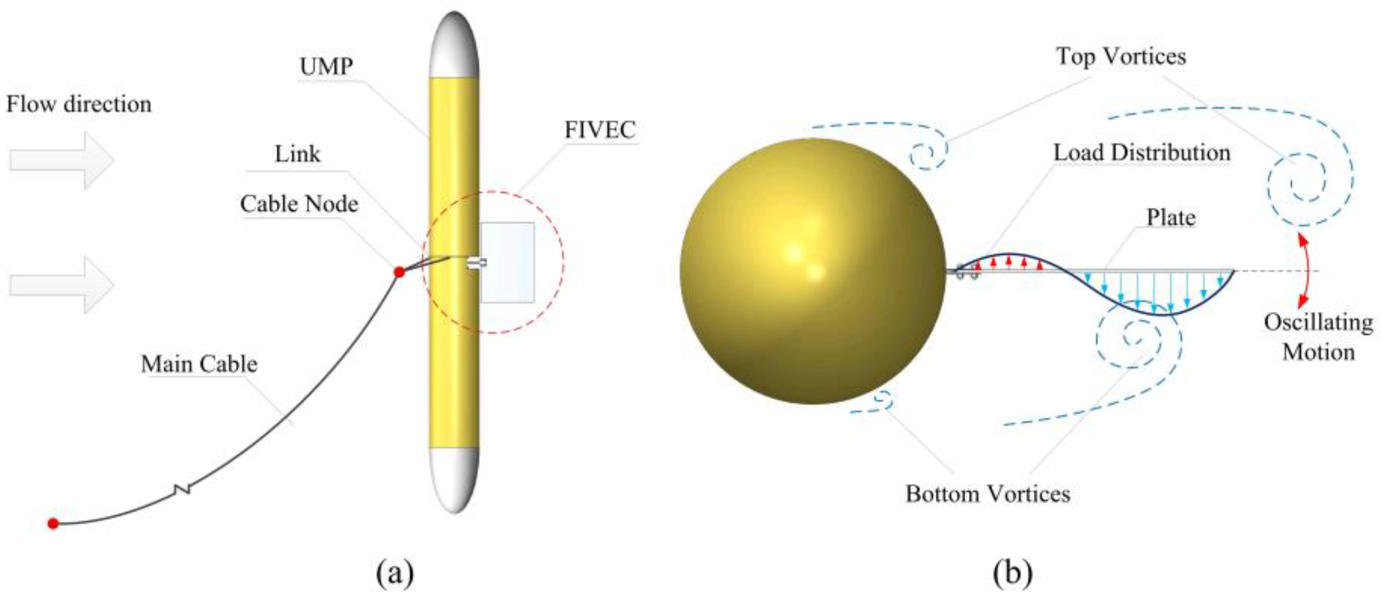
UMPs usually have blunt sections, so they will possibly experience vortex shedding on the surface. Inspired from the above research, the shed vortices from the UMP contain a certain kinetic energy and could possibly be recovered to provide power for the UMP. A vortex-induced vibration energy converter (FIVEC) for UMPs is then designed. Figure 1a shows the schematic diagram of the UMP and the FIVEC. The UMP is tethered to the seabed by a main cable, which is connected to a link of the UMP. The function of the link is shifting the anchored point on the UMP and increasing the motion stability. A thin plate is used to collect kinetic energy from the vortices. The working principle of the FIVEC is shown in detail in Figure 1b. At a certain Reynolds number, repeating vortices will shed from both sides of the cylinder [26]. The counter-rotating vortices will then change the load distribution on the plate periodically and drive the plate to vibration. This vibration motion will be transmitted to the inside of the FIVEC for power generation. A detailed description of the device will be given in Section 2.
The FIVEC is more suitable for UMPs than OCTs due to the much simpler structure. However, its performance has never been studied before. This paper will focus on evaluating the characteristics of motion, force, power, and flow structure of the FIVEC at different design parameters with a computational fluid dynamic (CFD) method. It should be noted that the working principle of the FIVEC design is similar to the thrust foils in turbulent wakes [27,28]. Shao and Pan numerically modeled a thrust foil in the wake of a D-cylinder [27], they found that the thrust of the foil was increased in the wake and explained the interactions between the vortices and the foil position. Similarly, Beal et al. investigated the hydrodynamics of a dead fish and a thin plate in the turbulent wake of a D-cylinder [28]; they found that the dead fish and the thin plate could generate thrust, lift and, most interestingly, mechanical energy from the vortices in the wake of the cylinder. These studies prove the feasibility of energy extraction from the vortices and give inspiration to the current research.
2. FIVEC Design
The FIVEC is designed to work in ocean currents, therefore, underwater sealing becomes an inevitable problem. With respect to underwater sealing, mechanical seals are commonly applied on the shafts to avoid the seepage and corrosion of the seawater. However, the mechanical seal increases the friction torque, which is harmful to the energy harnessing efficiency. In order to reduce the resistive torque brought by the mechanical seal, a magnetic coupling (MC) is used for the non-contacting transmission of torque. Figure 2 shows the components of the FIVEC design. The device is mainly composed of a plate, a MC, a sealed chamber, a volute spring, and a generator. The plate is used to generate torque from the wake of the UMP hull. The MC works to transmit the torque on the plate to the shaft inside the sealed chamber. The MC is composed of an outer magnetic rotor, an isolation hood, and an inner magnetic rotor. The outer rotor is connected to the plate and the inner rotor is connected with the volute spring. The isolation hood is located between the two magnetic rotors and forms a sealed chamber which contains the inner rotor, the spring, the gearbox, and the generator. Since the MC allows torque to transfer between the magnetic rotors using magnetic forces, the torque on the plate can be transmitted to the inner rotor without a contacting mechanical connection. The volute spring is used to adjust the natural frequency of the oscillating plate. The plate generates higher torque when its natural frequency is resonant to the vortex-shedding frequency on the UMP. The designed FIVEC has a compact structure and can be installed on existing UMPs as an independent component.
3. Mathematical Model
3.1. Geometric Model Simplification
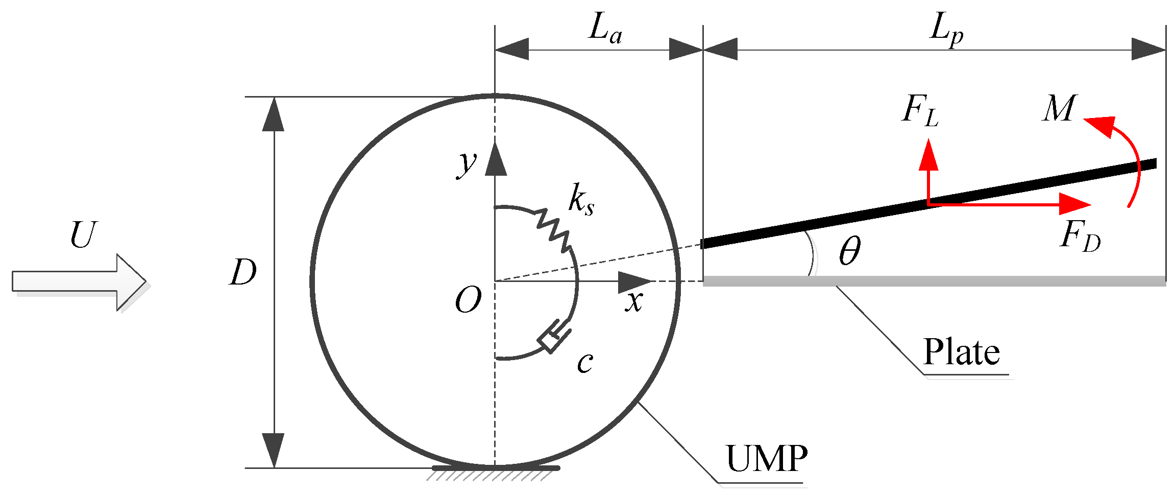
Since the plate has a uniform section shape in the spanwise direction, the model can be simplified with a two-dimensional approach. Two-dimensional models are generally utilized in the simulations of oscillating cylinders due to the smaller number of grids and less computational time [9,14,20,24]. Figure 3 presents a schematic of the two-dimensional model, where U is the velocity of the upstream flow, D is the diameter of the UMP, ks is the spring stiffness, c is the system damping, Lp is the length of the plate, θ is the rotation angle of the plate and La is the distance between the center of the UMP and the root of the plate. The UMP considered here has a diameter of D = 0.533 m and a small gap (La = 0.290 m) exists between the plate and the UMP to allow the free rotating of the plate. A typical flow velocity of U =1 m/s is selected for all simulations in this paper. It should be noted that the coupled motion of the UMP with FIVEC is very complicated in real-life situations. In this paper the UMP is assumed to be fixed and only the one degree-of-freedom (DOF) rotating motion of the plate is considered. Although this simplification may cause some deviations, it is a good start for the study of UMP vibration energy recovery. The results will also be useful for fixed cylinder situations, such as vibration energy recovery from ocean risers and the piles of tidal turbines.
3.2. Governing Equations and Turbulence Model
The governing equations are given by the incompressible form of the Navier-Stokes equations, including the continuity equation and momentum equation [29], as shown below:
in which:
where represents the velocity component in the i direction, is the fluctuation velocity component in the i direction, is the Cartesian coordinate in the i direction, t is time, p is pressure, and are density and kinematic viscosity of the fluid, respectively, is the turbulent viscosity, and k is the turbulent energy.
The SST k-ω turbulence model, which solves the kinetic energy (k) and its specific dissipation rate (ω), is applied for closing the RANS equations [29]. The SST k-ω model is a hybrid model combining the k-ω and the k-ε models. A blending function activates the k-ω model near the wall and the k-ε model in the free stream. This ensures that the appropriate model is utilized throughout the flow field. The SST k-ω turbulence model can give good predictions of the boundary layer flows with adverse pressure gradients, more detailed information on this model can be found in [30].
3.3. Equations of Motion
The 1 DOF dynamic equation of the oscillating plate is modeled via the classical mass-spring-damper system and can be presented as
where J is the total rotational inertial of the plate per unit length, c is the system damping, ks is the stiffness of the spring, θ is the oscillating angle of the plate, M is the hydrodynamic torque on the plate and the dot notation means the derivative with respect to time.
The total rotational inertial, J, is the sum of the plate structural rotational inertial, Jb, and the added mass component, Ja. The added mass is caused by the acceleration of a body in fluid. The empirical equations for the calculation of the structural rotational inertial and the added mass of a rotating plate can be found in [31]. In this paper, Ja and Jb can be calculated by the following equations:
where is the density of the plate and h is the thickness of the plate with h = 0.002 m.
The instantaneous power extracted from the flow by the plate is the product of the instantaneous torque, , and the instantaneous angular velocity, :
and the averaged power during one oscillation cycle can be expressed as:
where T is the period of the oscillation motion, which varies with system parameters, such as ks, c, and Lp, and the inflow velocity.
The total hydrokinetic power in the upstream flow can be calculated by:
where H is the unit height of the plate.
Then, the coefficient of power, which is defined as the ratio of the device harnessed energy and the hydrokinetic power available in upstream flow, can be expressed as:
In order to eliminate the dimensional effects, the lift and drag (FL and FD, as shown in Figure 3, respectively) are normalized by dividing a virtual force which is the product of the dynamic pressure () and the reference area of the UMP ():
Similarly, the torque can be represented as:
It should be noted that the directions of the forces are defined in the coordinate frame, Oxy, in Figure 3. The lift is positive when pointing in the Oy direction, the drag is positive when pointing in the Ox direction, and the torque is positive when pointing counterclockwise.
4. Numerical Approach
4.1. Mathematical Model
The incompressible RANS equations are solved using a commercial software code, FLUENT 15.0 (ANSYS Inc, Canonsburg, PA, USA), and in order to realize the dynamic mesh in FLUENT, user-defined functions (UDF) are applied to solve the response of the fluid-structure coupling effects. The plate motion can be solved by the following steps:
- (1)
- Solve the RANS equations accompanied with the SST k-ω turbulence model and obtain the hydrodynamic forces acting on the plate;
- (2)
- Calculating the acceleration at current time step (n):
- (3)
- Update the velocity for the next time step (n + 1):where is the time step size;
- (4)
- obtain the rotational displacement for the next time step (n + 1) and updating the computation mesh:
- (5)
- Return to Step (1) if the simulation is not completed.
4.2. Computational Domain and Boundary Conditions
The computational domain selected is a rectangle with a width of 30D and a length of 45D. The UMP is placed in the symmetry axis of the top and bottom boundary and at a distance of 15D from the left boundary. As shown in Figure 4, the overall domain is split into three subdomains, including an oscillating domain, an inner stationary domain, and an outer stationary domain. The oscillating domain has a ring shape and contains the cells around the plate. The inner stationary domain contains the cells around the UMP while the outer stationary domain contains the elements in the outer region. The rotational domain is separated from the other two stationary domains by two sliding interfaces. Using this segmentation method, the updating of local mesh in each time step is no longer needed and the mesh quality can be enhanced. The boundary conditions include:
- (1)
- Inlet: Uniform and steady velocity of 1 m/s;
- (2)
- Outlet: Pressure outlet with relative atmospheric pressure of 0 Pa;
- (3)
- Interface: The overlapped edges between the three domains are set as interfaces;
- (4)
- No slip wall: No slip wall conditions are imposed at the surfaces of the UMP and the plate; and
- (5)
- Sliding wall: Sliding wall conditions are imposed at both the top and the bottom edges.
4.3. Mesh Generation
All three domains are discretized with quadrilateral elements. Prism layer grid elements are extruded from the surfaces of the UMP and the plate to improve the grid quality and to provide sufficient precision to describe the boundary layer flow. The height of the first prism layer above the surfaces of the UMP and the plate is set so that the y+ value for the first layer of elements from the surfaces is around 1. The y+ value is a non-dimensional height of the grid determined by the size of the grid and Reynolds number. y+ = 1 is suggested by the Fluent User’s Guide [29] for the use of the SST k-ω turbulence model. Grid node density is higher near the UMP and the plate than in the other regions. The grid is created so that the control volumes are finer near the walls and coarser towards the boundaries. A sliding mesh method is used to simulate the oscillating of the plate. Figure 5 shows the meshes for two rotation positions, the oscillating domain rotates along the interfaces and about the center of the UMP without changing the local mesh.
4.4. Numerical Method Validation
A mesh independence verification study is conducted using three grids with different nodes densities (41,000/66,900/97,000 elements). The verification simulations are conducted at k = ∞, c = ∞, and Lp = D. The mesh independence is tested by assessing the root mean square (RMS) of the lift coefficient and the mean drag coefficient of the plate for different mesh densities. The results are summarized in Table 1. Both the Clp and Cdp have good consistency for different mesh densities. Accordingly, the mesh with medium density can predict the performance of the plate with sufficient accuracy and will be used in the later simulations.
To verify the accuracy of the CFD method in this paper, the results are compared with the experimental data of a 1-DOF transverse VIV circular cylinder presented by Liu et al. at Tianjin University [32]. The testing parameters adopted in the validation simulations are the same with the experiments and are listed in Table 2. The velocity is presented in a non-dimensional ratio:
where fn is the natural frequency of the device, fosc is the oscillation frequency and St is the Strouhal number that a dimensionless number generally used in describing oscillating flow mechanisms.
Figure 6 shows the comparison of the amplitude and frequency response between the numerical and the experimental results. The amplitude is the maximum transverse displacement of the cylinder caused by the vortex. It is observed that the VIV amplitudes obtained from the numerical method are in good agreement with the experimental data. The lock-in of the amplitude, which means that the amplitude is nearly unchanged, is well characterized in the upper branch (pointed out in Figure 6). A slight overestimate of the amplitude occurs at high flow velocities. As for the frequency, the numerical results agree with the experimental results well. It should be noted that the Strouhal number for these validation simulations is nearly constant and close to 0.2, this finding was also observed in a previously research done by Achenbach and Heinecke [33]. Therefore, the comparison with experiments shows that the numerical method is credible and acceptable.
5. Results and Discussion
The output power performance of the FIVEC is significantly influenced by the design parameters c, ks, and Lp, among which c determines the portion of the total power transformed into kinetic energy, ks affects the natural frequency of the plate, and Lp affects the rotational inertial and hydrodynamic forces. A previous study [21] has found that the VIV reaches the highest power harnessing efficiency when the oscillation frequency (fosc) is close to the device natural frequency (fn) and that the frequency ratio between the fosc and the fn is not affected significantly by the total damping. Therefore, the effects of k on the performance of the device are not considered and the specific value of ks is set so that fn is equal to the vortex shedding frequency according to: .
Since the appropriate values of c and Lp for the best power performance are unknown for this new design, this research takes the following steps to investigate the effects of the two parameters:
- (1)
- Perform simulations on fixed plates (ks = ∞, c = ∞) with different Lp, and find the rough range of Lp where stronger hydrodynamic forces occur. In addition, obtain the approximate frequency of the varying forces (f0);
- (2)
- Select a constant Lp in the rough range, calculate the rotational inertial according to Equations (5) and (6). Then define a constant ks to make fn, obtained by Equation (17), match with f0. Perform simulations for the specific Lp and ks and study the response of the system with different c; and
- (3)
- Select an optimal c based on the results of Step (2), evaluate the system performance when Lp varies. In this simulation group, ks varies for each case so that the natural frequency fn is unchanged and matches with f0.
5.1. Results for the Fixed Plates
5.1.1. Instantaneous Forces
A series of simulations are carried out with Lp varying from 0 (without a plate) to 2.4D. The case of Lp = 1.5D is selected for the illustration of the instantaneous forces on both the UMP and the plate. The time history of the coefficients of forces, including the coefficients of torque, lift, and drag on the plate (termed as Cm, Clp, and Cdp, respectively) and the coefficients of lift and drag on the UMP (termed as Clu and Cdu, respectively), are shown in Figure 7a. To give a clear view, the curves of Clp, Cdp, and Clu are magnified by two, four, and 100 times, respectively. It can be seen that all the curves change irregularly at the beginning of the simulation and reach oscillatory convergence after 30 s. It should be noted that all the simulations in this research last for at least 50 s for the coefficients to reach convergence and the data in the last three cycles are used to calculate the averaged coefficients. The curves of torque and lift oscillate around zero and have an averaged zero value, while those of drag are biased. The Cdp curve offsets to the negative direction which means that the plate generates thrust rather than drag in the wake of the UMP. The plate is located behind the UMP and is influenced by the vortices shed from the UMP surface. The velocity direction of the vortices which contact with the plate surfaces points left, therefore, the plate generates negative drag, this phenomenon was also observed in an experiment of dead fish in vortices [28]. The Cdu remains at a high level of about 0.60 and shows a very slightly oscillation, as shown in the zoomed-in plot.
The fast Fourier transform (FFT) spectral analysis for the force coefficients are shown in Figure 7b. It is observed that the dominant frequencies are 0.4272 Hz for Cm, Clp, and Cdp, and is doubled (0.8545 Hz) for Cdp and Cdu. This indicates that the drag experiences two cycles in a whole plate oscillation cycle. Another finding is that Cdu has a second dominant frequency, 0.4272 Hz, which is the equal to the dominant frequencies of Cm, Clp, and Cdp. The reason for the two dominant frequencies of Cdu can be explained as follows: The first dominant frequency, 0.8545 Hz, is the result of the periodically shed vortices. The UMP in turn shed two contra-rotating vortices in a variation period (Figure 13, the flow structures will be discussed in depth in Section 5.2 and Section 5.3), each vortex has the same contribution to the drag, therefore, the frequency is twice that of the lift. The second dominant frequency, 0.4272 Hz, is the result of the interacting forces between the plate and the UMP and has the same frequency with that of the lift and torque.
5.1.2. Plate Length Effects
This section investigates the effect of length of the fixed plates on the force characteristics. To clearly characterize the forces on the UMP and the plate, the root mean square (RMS) of the lift and torque, and the averaged drag, are chosen in the following contents. The variation of the forces and their dominant frequency are shown in Figure 8.
The Clp increases with Lp/D from Lp/D = 0 to Lp/D = 1.0 and remains at a high level in the range of 1.0 < Lp/D < 2.0. As Lp/D further increases, a abrupt drop in Clp occurs. The Clu is greatly reduced in the region of 0 < Lp/D < 0.4, then increases slightly between 0.4 < Lp/D < 1.0. After that Clu decreases with the increased Lp/D and is almost zero after Lp/D = 2.2. Taking the total lift into consideration, the curve of the lift coefficient can be divided into three regions: a low suppression region (0 < Lp/D ≤ 1.0), a amplification region (1.0 < Lp/D ≤ 1.8), and a high suppression region (Lp/D > 1.8). In the two suppression regions, the total lift of the system is reduced, which means that the UMP vibration motion could be possibly suppressed. While in the amplification region, the total lift is higher than that of the bare UMP (Lp/D = 0), which means that a possible high output power of the blade could be obtained in this region. Therefore, a Lp/D of 1.0 is selected for the damping analysis in Section 5.2.
Since the lift and the torque has the same dominant frequency (Figure 7b), FFT frequencies of the Clp, alone, are used. The dominant frequency in Figure 8b is 0.5249 Hz for the bare UMP, and remains unchanged with a value of 0.4587 Hz between 0.1 ≤ Lp/D ≤ 1.4. A nearly linear decrease exists in the region of 1.5 < Lp/D ≤ 2.2. Although there must be a difference between the dominant frequencies of the fixed plate and the oscillating plate, the frequency of the fixed plate provides a guide for the design of the natural frequency of the oscillating plate. Since the dominant frequencies are very close when Lp/D varies from 0 to 1.4 and that the frequency may change slightly in the cases of oscillating plates due to the reaction of the plate on the UMP, a constant natural frequency of 0.5000 Hz is chosen for all the simulations in this study.
The Cdp shown in Figure 8c is rather smaller compared with the Cdu. This is because the plate is mainly influenced by the vortices rather than the freestream. Figure 9 presents the pressure contours and streamlines for three different fixed plates. It can be seen that the magnitude of the velocity around the plate is much lower than the freestream. In addition, the direction of the vortices on the plate surface is almost parallel to the plate, meaning that the pressure drag can be ignored. The Cdu decreases nearly linearly with increase of Lp/D. This is because the UMP with a plate has a more streamlined shape. The drag coefficients of streamlined shapes are smaller than that of the UMP, which has a circular section.
The Cm shown in Figure 8d rises with Lp/D from Lp/D = 0 to Lp/D = 1.7. It is easy to understand that the enlarged plate has a larger surface area and can generate a greater hydrodynamic torque. However, as Lp/D further increases, the Cm drops abruptly and remains at a low level after Lp/D = 2.2. This can be explained by the pressure contours in Figure 9. In the pressure contours of Lp/D = 2.2, the plate is too long and it is not easy for the reattached vortices to shed from the tip. As a result, both sides of the plate are covered by vortices and the pressure distributions are almost symmetrical. The torque on the plate is then greatly reduced.
5.2. Effects of Damping on the System Performance
Simulations are carried out with constant Lp (Lp = 1.0D) and ks (1020 N/rad, resulting with a natural frequency of 0.5000 Hz). The effects of c are evaluated over a range varying from 0 to 1000 Ns/rad.
5.2.1. Oscillation Amplitude and Power
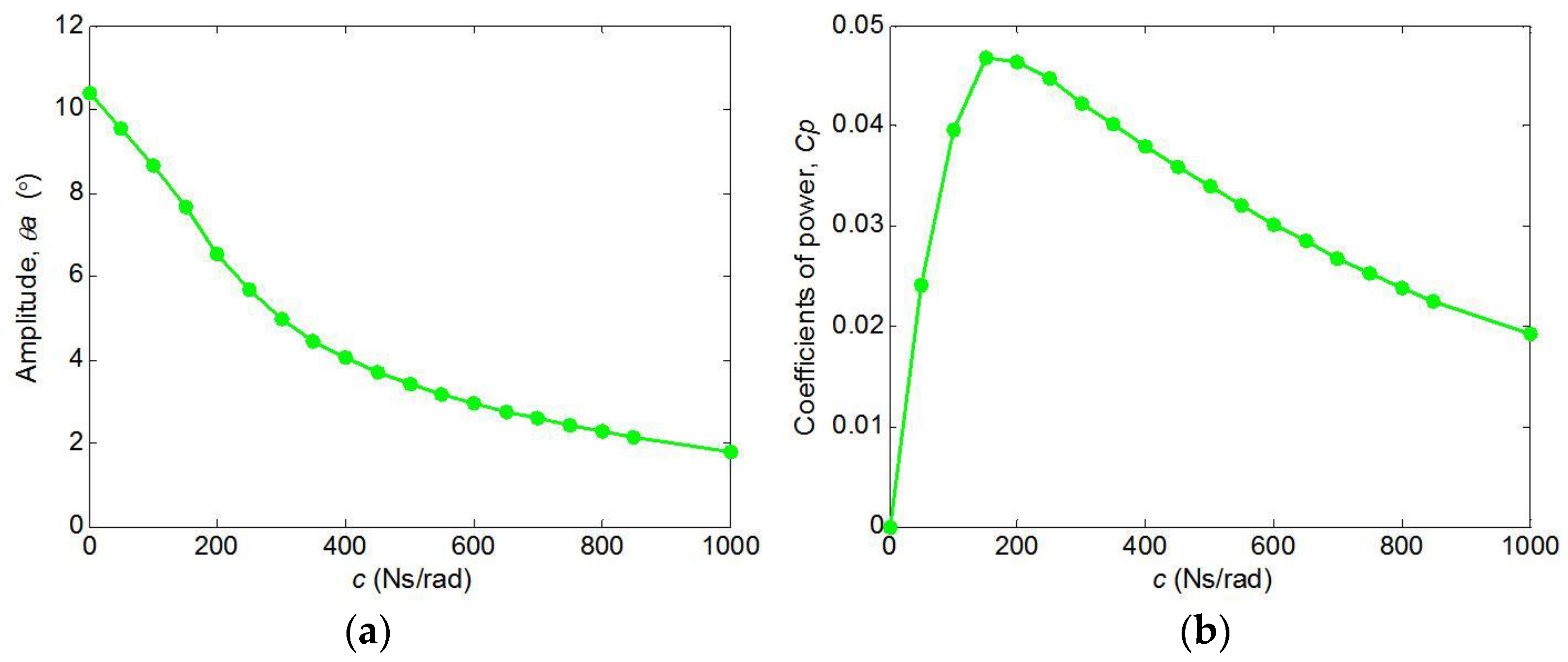
Figure 10 shows the variation of the oscillation amplitude, θa, and power coefficient, Cp, with respect to damping. θa decreases with the increase of c, due to the increased damping force which hinders the rotation of the plate. The maximum θa occurs at zero damping, with a value of 10.38°. Although the amplitude is higher for a smaller damping, the plate power is also smaller because it is proportional to c, according to Equation (7). As for p, it rises with c firstly to c = 150 Ns/rad, and then decreases with further increased c. The Cp has a peak value of 0.0482. This indicates that the suitable damping for high power output lies near c = 150 Ns/rad. Therefore, c = 150 Ns/rad is chosen for the plate length analysis in Section 5.3.
5.2.2. Performance of Forces
The RMS of the lift and torque coefficients, together with the averaged drag coefficients, are shown in Figure 11. Figure 11a suggests that the Clp increases with c for the whole examined range, but the growth rate decreases. It is known that the lift drives the plate while the damping force hinders the motion of the plate, so the plate with a higher damping is more capable to remain its position in flow. Therefore, the plate can generate a higher lift at a higher damping. Since the lift is the main force that generates the torque, the Cm shows a similar trend with the Clp, both increasing with c but decreasing in growth rate (Figure 11c).
The Clu decreases with c at first and reaches its minimum at c = 300 Ns/rad, then it increases slowly with c. An interesting finding is that the Clu is greatly reduced at c = 300 Ns/rad, causing the total lift coefficient to drop to 0.3549, which is 4.83% lower than that of a bare UMP (0.3729). To explain the variation of Clu, the instantaneous lifts of both the UMP and the plate are shown in Figure 12. There is a phase difference between the Clu and the Clp which makes the Clp lag behind the Clu. It is clearly shown that the phase difference increases with the damping. Since Clp is the main force that generates torque and drives the rotation of the plate, the phase difference leads to an asynchronization in the UMP lift and the plate motion. Figure 12 also shows the pressure contours around the UMP at t = 40.96, which corresponds to the maximum Clu. It is clear that the position of the plate differs at different damping. The rotation of the plate changes the flow near the suction (downstream) side of the UMP and affects the pressure on the UMP, as marked in the dotted circles. At c = 300 Ns/rad, the pressure on the UMP is almost symmetry about the centerline, so the Clu is greatly reduced. While for the other cases, the pressure on the top caused by the vortex shedding is lower than that on the bottom, so the Clu is relatively higher.
The Cdp is negative and near zero for all damping, this means that the plate could generate a small thrust in the wake. The total drag coefficient decreases with damping slightly at the beginning and then remains nearly constant after c = 400 Ns/rad. Generally, damping has only a slight effect on the drags of the UMP and the plate, because the amplitude of the plate is relatively small.
5.2.3. Wake Structures
In order to show the influences of system damping on the wake of the UMP, the time-varying coefficients of torque, Cm, and the angular position, θ, are presented in Figure 13. Three different c, including 0 (free motion), 150 Ns/rad (peak Cp) and 300 Ns/rad (high damping), are selected. It can be seen that the Cm curves show stronger oscillations at high damping, while the θ curves shows the opposite trend. Another finding is that a phase difference exists between Cm and θ, making Cm lags behind θ. This phase difference becomes more obvious at higher damping. Contours of vorticity are plotted at four typical points in a cycle of the Cm curve, as shown in the curves. The wake structure are similar for different damping. A regular 2S vortex pattern (two single vortices shed per cycle) is observed for all simulation cases. Two vortices are shed per cycle of oscillation, the clockwise rotating vortex by the top shear layer and the counter-clockwise rotating one by the bottom shear layer. Both the vortex shedding frequency and the distance between two adjacent vortices are equal. Vortices shed from both sides of the UMP and then reattaches to the surface of the plate forming a thick shear layer flow. The shear layer extends to the tip of the plate and then separates and forms contra-rotating vortices. This separation delay phenomenon is also observed in a previous study [34].
5.3. Effects of Plate Length on the System Performance
Ten sets of simulations are carried out at constant system damping (150 Ns/rad), natural frequency (0.5000 Hz), and inflow velocity (1 m/s). The effects of Lp are evaluated over a range varying from 0.2D to 1.8D.
5.3.1. Oscillation Amplitude and Power
Figure 14 shows the variation of the oscillation amplitude, θa, and the power coefficient, Cp, with respect to Lp/D. θa increases with Lp/D quickly from Lp/D = 0.2 and reaches the peak at Lp/D = 0.9 with a value of θa = 7.82°. After that θa drops approximately linearly with Lp/D. The Cp shows a similar trend with θa. The peak Cp is 0.0520 at Lp/D = 0.7, which means that the plate can generate an averaged power of 13.86 W from the flow. Although the peak Cp is smaller than conventional VIV devices (0.37 by Ding et al. [14]) and ocean current turbines, this result is still satisfactory. Considering that the standby power of common underwater mooring buoys are on the order of tens to hundreds of milliwatts, the averaged power produced by the FIVEC could compensate for that.
5.3.2. Performance of Forces
In order to clearly show the performance of forces at different plate lengths, the RMS of the lift and torque coefficients, together with the averaged drag coefficients, are shown in Figure 15. Although the Clp increases with Lp on the whole, there is a relatively flatter region (0.4 < Lp/D < 1.2) where Clp shows small fluctuation. The Clu decreases with Lp at first and reaches its minimum at Lp/D = 0.7, then it increases slowly. The Cdp is negative and decreases with the increase of Lp for all cases. The Cdu is increased slightly when Lp/D < 0.7 and drops nearly linearly with further increased Lp. While for the Cm, it shows a similar trend with the total Cl, both have little change within the region of 0.4 < Lp/D < 1.2.
In order to show the influences of plate length on the performance of the device, the time-varying coefficients of lift and amplitude are presented in Figure 16. Typically, four different lengths of plates, including 0 (bare UMP), 0.2D, 0.7D (corresponding to the peak Cp), and 1.4D, are selected and compared. Despite for the amplitude, the shapes of the curves of Clp and Clu are also different for different plate lengths. For Lp/D = 0 and 0.2, the curves are like rough sinusoidal curves, while for the other two cases, the curves are more complicated. Additionally, a phase difference exists between Clp and Clu, which is larger for longer plate lengths. Contours of vorticity are plotted at four typical points in a cycle of the Cm curve, as shown in Figure 14. The wake shows a regular 2S vortex pattern for all cases. This indicates that the plate have little effect on the far wake of the UMP. However, the near wake of the UMP is greatly influenced. The vortices shed from the UMP reattaches to the plate. The shear layer is then extended to the tip of the plate. The shifts in the shear layer are the reason for the variation of the forces.
To illustrate how Lp influences the forces on the UMP and the plate clearly, the velocity contours with streamlines and the pressure contours near the FIVEC are shown in Figure 17. The plate has three main effects on the near wake flow of the UMP. Firstly, the plate works as a barrier and prevents the vortices from rolling from one side to the other side of the UMP. It is clear to see that a vortex shed from the top of the UMP and rolls to the bottom, covering most area of the suction (downstream) surface at Lp/D = 0. This vortex significantly influences the flow near the bottom of the UMP and the pressure is recovered. The pressure difference between the top and the bottom side is then increased and, finally, the lift is increased. For the other cases with plates, the top vortices cannot easily move from the top to the bottom and the pressure on the bottom side of the UMP is hardly changed. This helps reduce the lift of the UMP. Secondly, the plate helps extend the length of the shear layer and delaying the shedding of vortices. The vortices separate from the tip of the plate and help extend the low-pressure area where separation occurs. Therefore, the pressure on the suction side of the UMP is increased and the drag is reduced. Thirdly, the push-and-pull movement of the plate causes a local flow near the suction side of the UMP, this flow is stronger at larger lengths of plate. Taking the case of Lp/D = 1.4 for example, the plate is rotating counterclockwise, pushing the flow on the top and drawing the flow at the bottom. Therefore, the pressure on the bottom side of the UMP is much smaller than the other cases. The effects of local flow is the reason for why Clu is increased at higher Lp/D.
6. Conclusions
In this paper, the design of a FIVEC for the energy supply of UMPs is proposed, which could possibly extend the operating time of UMPs. Two-dimensional CFD simulations are carried out on the novel device to evaluate its performances under various situations. Typically, two key design parameters, including the plate length and the system damping, are considered in the simulations. The effect of the length of the fixed plate on the forces and the vortex shedding frequency on the UMP is firstly studied. The reasons for the variation of the forces and the vortex shedding frequency are explained with the aid of flow structure distributions. Then, simulations are performed on a specific length of plate and at different dampings to find the optimal damping corresponding to the optimal power. Finally, the effect of the length of movable plate on the performance of the device is studied. The results show that the device could generate sustained power so that the feasibility of this design is proved. Some important conclusions of this study are summarized below:
- (1)
- The device characterizes with a maximum averaged power coefficient of 0.0520, corresponding to a power of 13.86 W at an inflow velocity of 1 m/s;
- (2)
- With the increase of damping, the oscillation amplitude decreases all the time while the power coefficient increases, at first, and then reduces after the peak value. The optimal damping for the best power performance is around 150 Ns/rad;
- (3)
- With the increase of plate length, both the oscillation amplitude and the power coefficient increases at first and then reduces after the peak value. The optimal plate length for the best power performance is around 0.7D; and
- (4)
- The plate has three main effects on the flow structure and the hydrodynamic forces of the UMP. First, it prevents the vortices from rolling from one side to the other side of the UMP. Second, it helps extending the length of the shear layer and delaying the shedding of vortices. Third, it causes a local flow near the suction side of the UMP.
Acknowledgment
This research was supported by the National Science Foundation of China (grant Nos. 51179159, 61572404) and the Fundamental Research Funds for the Central Universities.
Author Contributions
Wenlong Tian and Zhaoyong Mao conceived the idea; Wenlong Tian and Fuliang Zhao performed the simulations and analyzed the data; Wenlong Tian, Zhaoyong Mao and Fuliang Zhao drafted the paper; Wenlong Tian, Zhaoyong Mao and Fuliang Zhao approved the final version to be published; Wenlong Tian, Zhaoyong Mao and Fuliang Zhao agreed to be accountable for all aspects of the work in ensuring that questions related to the accuracy or integrity of any part of the work are appropriately investigated and resolved.
Conflicts of Interest
The authors declare no conflict of interest.
References
- Crimmins, D.; Patty, C.; Beliard, M.; Baker, J. Long-Endurance Test Results of the Solar-Powered Auv System. In Proceedings of the OCEANS 2006 on Conference Long-Endurance Test Results of the Solar-Powered AUV System, Boston, MA, USA, 18–21 September 2006; pp. 1–5. [Google Scholar]
- Wang, L.; Isberg, J. Nonlinear Passive Control of a Wave Energy Converter Subject to Constraints in Irregular Waves. Energies 2015, 8, 6528–6542. [Google Scholar] [CrossRef]
- Naty, S.; Viviano, A.; Foti, E. Wave Energy Exploitation System Integrated in the Coastal Structure of a Mediterranean Port. Sustainability 2016, 8, 1342. [Google Scholar] [CrossRef]
- Yang, X.; Haas, K.A.; Fritz, H.M. Theoretical Assessment of Ocean Current Energy Potential for the Gulf Stream System. Mar. Technol. Soc. J. 2013, 47, 101–112. [Google Scholar] [CrossRef]
- Gil, A.; Medrano, M.; Martorell, I.; Lázaro, A.; Dolado, P. State of the Art on High Temperature Thermal Energy Storage for Power Generation. Part 1—Concepts, Materials and Modellization. Renew. Sustain. Energy Rev. 2010, 14, 31–55. [Google Scholar] [CrossRef]
- Gerstandt, K.; Peinemann, K.V.; Skilhagen, S.E.; Thorsen, T.; Holt, T. Membrane processes in energy supply for an osmotic power plant. Desalination 2008, 224, 64–70. [Google Scholar] [CrossRef]
- Hu, Y.; Wang, J. Study on Power Generation and Energy Storage System of a Solar Powered Autonomous Underwater Vehicle(SAUV). Energy Procedia 2012, 16, 2049–2053. [Google Scholar]
- Huang, Y.M.; Hush, J.C.; Wang, K.J. Design of a Remote Controlled Solar Powered Boat. In Proceedings of the ASME 2006 International Mechanical Engineering Congress and Exposition, Chicago, IL, USA, 5–10 November 2006; pp. 51–59. [Google Scholar]
- Kong, Q.; Ma, J.; Xia, D. NUMERICAL and experimental study of the phase change process for underwater glider propelled by ocean thermal energy. Renew. Energy 2010, 35, 771–779. [Google Scholar] [CrossRef]
- Webb, D.; Simonetti, P.; Jones, C. Slocum: An underwater glider propelled by environmental energy. IEEE J. Ocean. Eng. 2001, 26, 447–452. [Google Scholar] [CrossRef]
- Tian, W.; Song, B.; Mao, Z. Conceptual design and numerical simulations of a vertical axis water turbine used for underwater mooring platforms. Int. J. Naval Archit. Ocean Eng. 2013, 5, 625–634. [Google Scholar]
- Tian, W.; Song, B.; Vanzwieten, J.H.; Pyakurel, P.; Li, Y. Numerical simulations of a horizontal axis water turbine designed for underwater mooring platforms. Int. J. Naval Archit. Ocean Eng. 2016, 8, 73–82. [Google Scholar] [CrossRef]
- Tian, W. Study on the Key Technologies of Hydrokinetic Current Turbines Designed for Underwater Moored Platforms; Northwestern Polytechnical University: Xi’an, China, 2016. (In Chinese) [Google Scholar]
- Ding, L.; Zhang, L.; Bernitsas, M.M.; Chang, C.C. Numerical simulation and experimental validation for energy harvesting of single-cylinder VIVACE converter with passive turbulence control. Renew. Energy 2016, 85, 1246–1259. [Google Scholar] [CrossRef]
- Rostami, A.B.; Armandei, M. Renewable energy harvesting by vortex-induced motions: Review and benchmarking of technologies. Renew. Sustain. Energy Rev. 2017, 70, 193–214. [Google Scholar] [CrossRef]
- Bernitsas, M.M.; Raghavan, K. Fluid Motion Energy Converter. U.S. Patent 7,493,759 B2, 24 February 2009. [Google Scholar]
- Bernitsas, M.M.; Ben-Simon, Y.; Raghavan, K.; Garcia, E.M.H. The VIVACE Converter: Model tests at high damping and Reynolds number around 105. J. Offshore Mech. Arctic Eng. 2009, 131, 403–410. [Google Scholar] [CrossRef]
- Bernitsas, M.M.; Raghavan, K. Enhancement of Vortex Induced Forces and Motion Through Surface Roughness Control. U.S. Patent 8,047,232 B2, 2 Novenber 2011. [Google Scholar]
- Chang, C.C.; Kumar, R.A.; Bernitsas, M.M. Viv and galloping of single circular cylinder with surface roughness at 3.0 × 10 4 ≤ Re ≤1.2 × 10 5. Ocean Eng. 2011, 38, 1713–1732. [Google Scholar] [CrossRef]
- Lin, D.; Li, Z.; Wu, C.; Mao, X.; Jiang, D. Flow induced motion and energy harvesting of bluff bodies with different cross sections. Energy Convers. Manag. 2015, 91, 416–426. [Google Scholar]
- Sun, H.; Kim, E.S.; Nowakowski, G.; Mauer, E.; Bernitsas, M.M. Effect of mass-ratio, damping, and stiffness on optimal hydrokinetic energy conversion of a single, rough cylinder in flow induced motions. Renew. Energy 2016, 99, 936–959. [Google Scholar] [CrossRef]
- Farshidianfar, A.; Zanganeh, H. A modified wake oscillator model for vortex-induced vibration of circular cylinders for a wide range of mass-damping ratio. J. Fluids Struct. 2010, 26, 430–441. [Google Scholar] [CrossRef]
- Gonçalves, R.T.; Rosetti, G.F.; Franzini, G.R.; Meneghini, J.R.; Fujarra, A.L.C. Two-degree-of-freedom vortex-induced vibration of circular cylinders with very low aspect ratio and small mass ratio. J. Fluids Struct. 2013, 39, 237–257. [Google Scholar] [CrossRef] [Green Version]
- Ding, L.; Zhang, L.; Kim, E.S.; Bernitsas, M.M. URANS vs. Experiments of flow induced motions of multiple circular cylinders with passive turbulence control. J. Fluids Struct. 2015, 54, 612–628. [Google Scholar] [CrossRef]
- Liu, Z.W.; Xiao-Hu, L.I.; Chen, Z.Q. Experiment of Aerodynamic Interference on Vortex-Induced Vibration of Two Rectangular Cylinders in Tandem in Smooth Flow Field. China J. Highw. Transp. 2010, 23, 44–50. [Google Scholar]
- Williamson, C.; Roshko, A. Vortex formation in the wake of an oscillating cylinder. J. Fluids Struct. 1988, 2, 355–381. [Google Scholar] [CrossRef]
- Xueming, S.; Yi, D. Hydrodynamics of a flapping foil in the wake of a D-section cylinder. J. Hydrodyn. 2011, 23, 422–430. [Google Scholar]
- Beal, D.N.; Hover, F.S.; Triantafyllow, M.S.; Liao, J.C.; Lauder, G.V. Passive propulsion in vortex wakes. J. Fluid Mech. 2006, 549, 385–402. [Google Scholar] [CrossRef]
- ANSYS. FLUENT 15.0 User’s Guide; ANSYS: Canonsburg, PA, USA, 2013. [Google Scholar]
- Menter, F.R. Two-equation eddy-viscosity turbulence models for engineering applications. AIAA J. 1994, 32, 1598–1605. [Google Scholar] [CrossRef]
- Yuwen, Z. Torpedo Shape Design; Northwestern Polytechnical University Press: Xi’an, China, 1998. (In Chinese) [Google Scholar]
- Liu, Z.; Liu, F.; Yan, X.; Zhang, J.; Tong-Sheng, B.U. Experimental Study of Cylinder Vortex Induced Vibration Under High Damping Ratio and Low Mass Ratio Conditions. J. Exp. Mech. 2014, 29, 737–743. (In Chinese) [Google Scholar]
- Achenbach, E.; Heinecke, E. On vortex shedding from smooth and rough cylinders in the range of Reynolds numbers 6E3 to 5E6. J..Fluid Mech. 1981, 109, 239–251. [Google Scholar] [CrossRef]
- Yun, Z.L.; Jaiman, R.K. Wake stabilization mechanism of low-drag suppression devices for vortex-induced vibration. J. Fluids Struct. 2017, 70, 428–449. [Google Scholar]
Figure 1.
(a) Schematic diagram (lateral view) and (b) working principle of the FIVEC (top view).

Figure 2.
Components of the FIVEC: (a) general view and (b) inside view.

Figure 3.
Schematic of the two-dimensional model.

Figure 4.
Domains and boundary conditions.

Figure 5.
Computing mesh at different rotation angles: (a) θ = 0°, and (b) θ = 15°.

Figure 6.
Comparison of amplitude and frequency responses between the numerical results and the experimental results.
Figure 6.
Comparison of amplitude and frequency responses between the numerical results and the experimental results.

Figure 7.
(a) Time history of the coefficients of forces; and (b) the frequency spectrum.

Figure 8.
Results for the fixed plate simulations.

Figure 9.
Pressure contours and streamlines for three different fixed plates.

Figure 10.
Effects of damping on (a) oscillation amplitude and (b) Cp.

Figure 11.
Effects of damping on (a) lift, (b) drag, and (c) torque.

Figure 12.
Instantaneous lifts and pressure contours around the UMP for different dampings.

Figure 13.
Wake structures for different system damping: (a) c = 0 Ns/rad, (b) c = 150 Ns/rad, and (c) c = 300 Ns/rad.
Figure 13.
Wake structures for different system damping: (a) c = 0 Ns/rad, (b) c = 150 Ns/rad, and (c) c = 300 Ns/rad.

Figure 14.
Effects of plate length on (a) oscillation amplitude and (b) Cp.

Figure 15.
Effects of plate length on (a) lift, (b) drag, and (c) torque.

Figure 16.
Wake structures for different plate lengths: (a) Lp/D = 0, (b) Lp/D = 0.2, (c) Lp/D = 0.7, and (d) Lp/D = 1.4.
Figure 16.
Wake structures for different plate lengths: (a) Lp/D = 0, (b) Lp/D = 0.2, (c) Lp/D = 0.7, and (d) Lp/D = 1.4.

Figure 17.
Velocity contours with streamlines (a) and pressure contours (b) for different plate lengths.
Figure 17.
Velocity contours with streamlines (a) and pressure contours (b) for different plate lengths.


Table 1.
Mesh convergence results.
| Mesh | No. of Elements | RMS of Cl | Averaged Cd |
|---|---|---|---|
| 1 | 41,000 | 0.3704 | −0.0015 |
| 2 | 66,900 | 0.3729 | −0.0013 |
| 3 | 97,000 | 0.3735 | −0.0013 |
Table 2.
Physical model parameters for the simulation.
| Description | Symbol | Value |
|---|---|---|
| Mass | m (g) | 152.75 |
| Damping | c (Ns/m) | 4.05 |
| Velocity ratio | 3–13 | |
| Spring stiffness per unit length | ks (N/m) | 13.77 |
| Diameter | D (mm) | 32 |
© 2017 by the authors. Licensee MDPI, Basel, Switzerland. This article is an open access article distributed under the terms and conditions of the Creative Commons Attribution (CC BY) license (http://creativecommons.org/licenses/by/4.0/).
Share and Cite
MDPI and ACS Style
Tian, W.; Mao, Z.; Zhao, F. Design and Numerical Simulations of a Flow Induced Vibration Energy Converter for Underwater Mooring Platforms. Energies 2017, 10, 1427. https://doi.org/10.3390/en10091427
AMA Style
Tian W, Mao Z, Zhao F. Design and Numerical Simulations of a Flow Induced Vibration Energy Converter for Underwater Mooring Platforms. Energies. 2017; 10(9):1427. https://doi.org/10.3390/en10091427
Chicago/Turabian StyleTian, Wenlong, Zhaoyong Mao, and Fuliang Zhao. 2017. "Design and Numerical Simulations of a Flow Induced Vibration Energy Converter for Underwater Mooring Platforms" Energies 10, no. 9: 1427. https://doi.org/10.3390/en10091427
Note that from the first issue of 2016, this journal uses article numbers instead of page numbers. See further details here.