Abstract
In this paper, the calculation of the conductor temperature is related to the temperature sensor position in high-voltage power cables and four thermal circuits—based on the temperatures of insulation shield, the center of waterproof compound, the aluminum sheath, and the jacket surface are established to calculate the conductor temperature. To examine the effectiveness of conductor temperature calculations, simulation models based on flow characteristics of the air gap between the waterproof compound and the aluminum are built up, and thermocouples are placed at the four radial positions in a 110 kV cross-linked polyethylene (XLPE) insulated power cable to measure the temperatures of four positions. In measurements, six cases of current heating test under three laying environments, such as duct, water, and backfilled soil were carried out. Both errors of the conductor temperature calculation and the simulation based on the temperature of insulation shield were significantly smaller than others under all laying environments. It is the uncertainty of the thermal resistivity, together with the difference of the initial temperature of each radial position by the solar radiation, which led to the above results. The thermal capacitance of the air has little impact on errors. The thermal resistance of the air gap is the largest error source. Compromising the temperature-estimation accuracy and the insulation-damage risk, the waterproof compound is the recommended sensor position to improve the accuracy of conductor-temperature calculation. When the thermal resistances were calculated correctly, the aluminum sheath is also the recommended sensor position besides the waterproof compound.
1. Introduction
XLPE (cross-linked polyethylene) insulated cable is currently a major type of high-voltage power cable, and its insulation condition is related to conductor temperature []. Since the conductor temperature of the in-service cable is difficult to measure directly, it is usually obtained by calculation. The IEC-60287 standard provides the general methods for determining the conductor temperature and current rating in cable, and the IEC-60853 standard provides the methods of cyclic-current rating when the thermal capacities of cable structures cannot be ignored [,]. These standards are used to calculate the conductor-temperature rise with environmental temperature and laying conditions according to the thermal circuit. The calculation result, however, usually exhibits errors because of the uncertainties of environmental parameters []. To solve this problem, many studies, including the modified thermal circuits and the numerical methods [,], have been undertaken. In numerical methods, the finite element method (FEM) is the most used method that has been applied to various laying environments. For example, the rating of underground cables []; cables in a tray []; the effects of radiation, solar heating, duct structures, and back-filled materials []; and, the formation of the dry zone around underground cables [] have been studied by FEM. Other numerical methods, including the finite difference method (FDM) [] and the boundary element method (BEM) [], have also been studied. The above numerical methods can generally model complicated laying conditions with high accuracy, but the thermal circuit is more suitable for meeting the demand of transient rating and online implementation [].
For engineering, the conductor temperature calculation of in-service cable is closely related to the temperature sensor. Typical arrangements of the sensor in a practical cable in studies are given in the following Table 1 [,,,,,].

Table 1.
Radial positions of the sensor in practical cables.
In these cases, when the sensor has realized the temperature measurement of a certain structure, the real-time conductor temperature could then be obtained according to the corresponding thermal circuit [], or using the numerical methods, like FEM []. There are various placements available for the sensor, except the conductor and the solid insulation layers, from the perspective of manufacture, and the principle of determining the position of temperature sensor is still unspecified. Therefore, the effect of the different detection positions on the conductor-temperature calculation needs to be researched to optimize the temperature-sensor arrangement, and then a better calculation accuracy could be achieved on the premise of ensuring the insulation security.
When calculating the conductor temperature, the thermal parameters of the substantial materials in standards are usually used for the entire thickness between conductor and jacket []. However, the heat transport may be more complex for the cable that has a substantial volume of air under the corrugated metal sheath []. Generally, the methods to take this air gap into account included adding an empirically derived constant, which was not found in standards, to the calculated thermal resistance. In addition, when considering the in corrugation designs difference, and the clearance variation that is caused by the thermal expansion and contraction of the materials inside the sheath, it is difficult to recommend a constant for modification []. Two main thoughts are available to handle the air gap. One is to follow the way of calculating the thermal resistance and capacitance in standards, the other is considering the flow characteristics and solving the thermal field, which has also been used in other power equipment []. The first way is simplified by using the appropriate correlations when we mainly focus on its heating power rather than the flow characteristics, so the flow regimes, including the laminar and turbulent flow, could be handled at a very low computational cost. The second way solves for both the total energy balance and the flow equations of the air, which produces detailed results for the flow field, as well as for the temperature distribution and heating power, but it is more complex and requires more computational resources and time than the first approach. Therefore, the handling of the air inside the cable requires more attention.
To determine the appropriate radial position for the temperature sensor in the cable and determine the factors influencing the conductor-temperature calculation, in this paper, we took XLPE power cable as an example and established thermal circuits based on the temperatures of the insulation shield, the center of waterproof compound, the aluminum sheath, and the jacket surface. Thermocouples were arranged in the above radial positions of a 110 kV single-core XLPE power cable, and six cases of current heating experiment under three laying environments, including duct, water, and backfilled soil, were carried out. The real-time conductor temperature was calculated according to the current and the measured temperature, and then the effect of radial positions on conductor temperature calculations was analyzed. In addition, FEM was used to validate the accuracy of the calculation by considering both the effects of convection and radiation in the air layer of cable. All of the factors influencing the conductor-temperature calculation, including the thermal resistance and thermal capacitance, and the initial temperature, were discussed. Thus, a referential radial-position for the arrangement of temperature sensor was proposed.
2. Conductor Temperature Calculation Methods Based on Different Radial-Position-Temperatures
2.1. Principle of Thermal Circuits
The analytic temperature-distribution calculation in power cables generally ignores the axial heat transfer, and uses the lumped parameters to describe parts of the cable itself, as well as the surrounding environment in the direction of radius, and the ladder thermal circuit is established. As for the transient heat-transfer process, a thermal capacitance parameter is introduced to describe the heat-storage model, which is shown in Figure 1a. Figure 1b shows a simplified arrangement of the thermal capacitance of the layer, as proposed by Van Wormer [], who used an equivalent π thermal circuit to express the heat-transfer process.
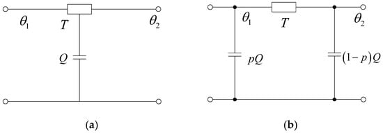
Figure 1.
Lumped parameter model of a cylinder layer: (a) before equivalence and (b) the equivalent π circuit.
In Figure 1, thermal resistance T, thermal capacitance Q, and allocation factor p could be calculated, respectively, using the following equations:
where ρT is the thermal resistivity in (K·m)/W, D and d the external and internal diameter of the layer in m, and σ the volumetric specific heat in J/(m3·K).
T = ρTln(D/d)/(2π),
Q = σπ(D2 − d2)/4,
p = 1/(2ln(D/d)) − 1/((D/d)2 − 1),
In Figure 1, the power loss in the conductor, the dielectric loss and the sheath loss should be considered. The conductor loss can be calculated according to:
where WC represents the power losses of conductor and sheath per unit length in W/m, I the current in A, and R the ac resistance of the conductor in Ω.
WC = I2R,
When the voltage has been applied on the cable over a long period of time, the temperature rise that is caused by dielectric loss could be regarded as stable, so that the transient temperature rise of the conductor usually only takes the current heating into account, and the dielectric loss is ignored. The sheath loss is usually merged into the nearby thermal resistance and capacity, via a partition coefficient qs, which is calculated using []:
where λ1 is the ratio of sheath loss to the power loss in the conductor.
qs = 1 + λ1,
2.2. Thermal Circuit Calculation Methods of Conductor Temperature Based on Four Radial Position Temperatures
Having investigated the structural features of an actual power cable, the insulation-shield surface, the center of waterproof compound, the aluminum sheath, and the jacket surface, are the available locations for the placement of temperature sensors. The thermal circuit with the temperatures of different radial positions is given in Figure 2. Apparently, all of these temperature calculation methods are of a similar circuit, but different in their boundary conditions.
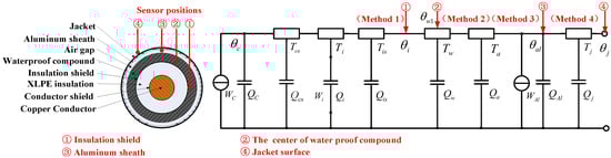
Figure 2.
Radial positions of temperature sensor and corresponding thermal circuit in a cable.
The thermal conductivities of the copper conductor and the aluminum sheath are much greater than those of the other material, such that these two structures could be regarded as isothermal surfaces. In Figure 2, Wal denotes the power losses of the sheath per unit length in W/m. Tcs, Ti, Tis, Tw, Ta, and Tj are, respectively, the thermal resistances of the conductor shield, insulation, insulation shield, waterproof compound, air gap, and jacket in (K·m)/W. Q, Qcs, Qi, Qis, Qw, Qa, Qal, and Qj are, respectively, the thermal capacitances of the conductor, conductor shield, insulation, insulation shield, the center of waterproof compound, air gap, aluminum sheath, and jacket in J/(m3·K). θc, θi, θw1, θal, and θj are, respectively, the temperatures of the conductor, insulation shield surface, waterproof compound center, aluminum sheath, and jacket surface in °C. In addition, the environmental temperature is represented by θe.
According to Figure 2, a transient temperature-calculation model from insulation shield to conductor was first developed after referring to the standard method for a short duration in IEC-60853 when the current and the temperature of the insulation shield were known, which is denoted Method 1. Since the thicknesses of the conductor shield as well as of the insulation shield are very low, and their thermal characteristics are similar to that of XLPE insulation, these two structures are usually merged into the insulation layer to simplify the calculation []. The thermal resistance and the thermal capacitance of the insulation layer were partitioned at the geometric average of its internal and external diameter, and then the thermal capacitances were partitioned to both sides of thermal resistances by the allocation factor shown in Figure 1. The transient model was finally simplified to be a two-loop network, as illustrated in Figure 3, where θb is the boundary condition that represents the temperature of the insulation shield in Method 1, TA and TB are the equivalent thermal resistances, and QA and QB are the equivalent thermal capacitances []. According to Figure 3, the temperature rise of the conductor relative to the insulation shield, θ(t), could be obtained by:
where a, b, Ta, and Tb are determined by TA, TB, QA, and QB [].
θ(t) = Wc(Ta(1 − exp(−at)) + Tb(1 − exp(−bt))),
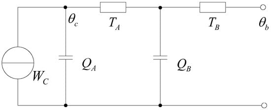
Figure 3.
Simplified transient thermal circuit model from insulation shield to conductor.
As for the conductor temperature inverted from the temperatures of the center of the waterproof compound, aluminum sheath, and jacket surface, simplified transient thermal circuits from the corresponding radial positions to the conductor were established and marked as Methods 2, 3, and 4, respectively. All of the thermal capacitances that are involved in the transient model were partitioned to both sides of the thermal resistances by the allocation factor in the same way, and the sheath loss was merged into the nearby thermal resistance and capacity parameters via qs. Thus, we obtained the ladder network shown in Figure 4, where the boundary temperature θb represents θw1 in Method 2, θal in Method 3, and θj in Method 4, respectively. Tα to Tν and Qα to Qν represent the equivalent thermal resistances and thermal capacitances within the boundary.
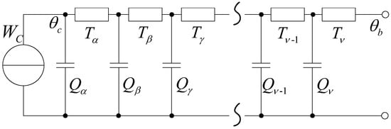
Figure 4.
Transient thermal circuit model from boundary to conductor.
Figure 4 could be simplified to the two-loop network shown in Figure 3 [], according to:
TA = Tα,
QA = Qα,
TB = Tβ + Tγ + Tδ +…+ Tν−1 + Tν,
QB = Qβ + ((Tγ + Tδ +…+ Tν)/(Tβ + Tγ +…+ Tν))Qγ +
((Tδ +…+ Tν)/(Tβ + Tγ +…+ Tν))Qδ +…+ (Tν/(Tβ + Tγ +…+ Tν))Qν
((Tδ +…+ Tν)/(Tβ + Tγ +…+ Tν))Qδ +…+ (Tν/(Tβ + Tγ +…+ Tν))Qν
When the boundary temperature as well as the current were provided as solution conditions, the time-varying temperature θc(t) could be obtained based on (6). As time goes by, the heat storage of thermal capacitance kept increasing, and a steady temperature distribution of the cable could be attained after a long enough period with constant current and ambient.
2.3. FEM Simulation Methods of Conductor Temperature Based on Different Radial Position Temperatures
The FEM simulation model for the cable was built in COMSOL Multiphysics (5.2a, COMSOL, Stockholm, Sweden). It consists of each layer in Figure 2. The main interest is to calculate the conductor temperature when the heating power and the boundary temperature are known. The cable has an initial temperature of ambient and heats up over time, due to Joule heating effect. The model is illustrated in Figure 5.
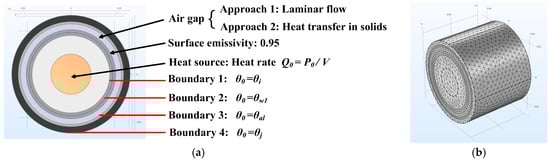
Figure 5.
Finite element method (FEM) simulation model: (a) conditions and (b) mesh generation.
The key problem is how to handle the air gap between the waterproof compound and the aluminum sheath. Two methods were applied to handle the natural convection heating of air. Approach 1 modeled the convective flow of the air directly, while in Approach 2, the thermal dissipation of the air was equivalent to the combination of thermal resistivity and heat capacity, as presented in standards. In this paper, we firstly used Approach 1 to simulate the temperature field of the cable to compare with the experimental results. Then, Approach 2 was adopted to study the correctness of each temperature calculation method.
The assumptions of the simulation are as follows. The model of solid heat transfer was used, and laminar flow was used to define the air structure when using Approach 1. The model solved a thermal balance for the cable structures, including the air flowing in the gap if needed. Thermal energy was transported through conduction in solid layers and through convention and radiation in the air layer. Taking surface-to-surface radiation between the waterproof compound and the aluminum sheath into account, the surface emissivity of the waterproof compound was set to 0.95.
The boundary conditions in the FEM model, were same to those in thermal circuit Methods 1, 2, 3, and 4 in Figure 2, and the insulation shield, the center of waterproof compound, the aluminum sheath, and the jacket surface, were denoted Boundaries 1, 2, 3, and 4, respectively. Heat rate was use to defined the heat source. The thermal conductivity, the heat capacity, and the density of the air, were temperature-dependent material properties. Other simulation conditions, including the control equations and the parameter of material, were predefined in the software automatically.
3. Experiments
3.1. Experiment Arrangement and Equipment
Current-heating experiments were performed on a 110 kV single-core XLPE insulated power cable, whose parameters are given in Table 2. The thermal resistivity and volumetric specific heat of the solid materials are recommended by IEC standards [,]. In addition, since it is difficult to recommended constants for the air between waterproof compound and aluminum sheath, the heat parameters of quiescent air were adopted [].
Table 2.
Parameters of the tested 110 kV single-core cross-linked polyethylene (XLPE) cable.
The experimental arrangement at Guangzhou Lingnan Cable Co., Ltd. (Guangzhou, China) is illustrated in Figure 6.
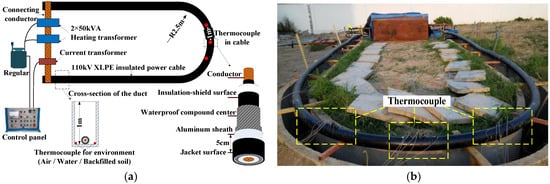
Figure 6.
Experimental arrangement: (a) diagram and (b) actual scene.
According to the test standard [], the tested cable, with a length of approximately 25 m, was bent into a U shape with a radius of 2.5 m. The ends of the cable were connected with a copper conductor and the aluminum sheath was not electrically grounded. When in water or backfilled soil, the cable was laid at a depth of 1 m.
In this experiment, high voltage was not applied and two 50 kVA heating transformers (CXBYQ-50, Xinyuan Electric Co., Ltd., Yangzhou, China) were used to generate an induction current of high intensity to the closed cable loop. The real-time current and conductor temperature were measured at the end of the tested cable to keep the output testing current basically stable by operating the regulator.
As shown in Figure 6, three groups of K-type thermocouples were symmetrically placed along the arc of the tested cable at an interval of 1 m. Each group consisted of five thermocouples that were inserted into the conductor, insulation shield, the center of waterproof compound, aluminum sheath, and jacket surface in sequence, with an interval of 5 cm in the axial direction. In addition, the ambient temperature was surveyed by the thermocouple placed at the bottom of the duct.
3.2. Experimental Scheme
The experiment schedule is given in Table 3.
Table 3.
Current heating experiment scheme.
The first two cases were carried out with the same constant current in the duct, and then four cases with different currents when the duct was filled with water or the backfilled soil. Each experiment began in a steady temperature condition without current being loaded, and the entire rising process from ambient temperature to steady-state temperature was recorded every 0.5 h. The experiments met the demand of the test standard [] that the temperature difference in the central area of 2 m should not exceed 2 °C, so the following calculation and analysis adopted the data of the center of the cable loop.
4. Results and Analysis
4.1. Comparison of the Experiments and Thermal Circuit Calculations Based on Different Radial-Positions
The results of six test cases are shown in Figure 7. Corresponding to four radial position temperatures, calculation results of conductor temperature based on thermal circuits are shown in Figure 8, where Methods 1–4 represent the conductor temperatures inverted from θi, θw1, θal, and θj, respectively, according to the models described in Section 2.
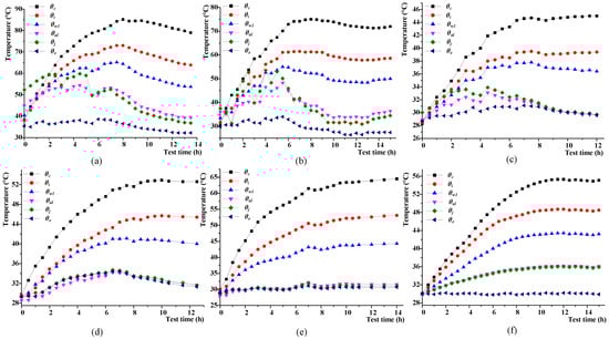
Figure 7.
Measured temperatures of different radial positions in the cable and environment: (a–f) represent Cases 1–6.
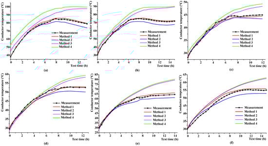
Figure 8.
Calculated conductor temperatures based on different radial-positions and the measured conductor temperatures: (a–f) represent Cases 1–6.
From Figure 7, the conductor, insulation shield, and the center of the waterproof compound basically exhibited the same temperature-variation tendency, while those of the jacket surface and the aluminum sheath were similar. Each case had recorded a gentle variation of temperature distribution, except for Cases 1 and 2. In these two cases, the cable was placed at the bottom of the duct and were exposed to the solar radiation in the daytime, which made the temperature variations of the jacket and aluminum sheath more violent. During the last several hours at midnight, the effect of the solar radiation disappeared, and the steady temperature gradients of the Cases 1 and 2 were similar because of the roughly identical conductor loss. However, both the ambient and the jacket surface temperatures in Case 1 were higher, so a higher boundary temperature of the cable resulted in higher temperatures in cable. When comparing Case 1 with Case 2, the steady temperature differences of five measuring points inside the cable ranged from 8.2 °C to 10.4 °C.
From Figure 8, similar tendencies in both the measurement and the calculation of conductor temperature were found in each case. In general, the calculation results based on Method 1 were closest to the measurements, and that of Method 2 was closer. However, a remarkable difference was found on the results based on Method 3 or 4.
To compare the effect of radial-position temperature detections on the accuracy of the conductor-temperature calculation, quantitative analysis was required. The absolute and relative errors of the calculation when compared to the measurement are defined as:
where θc and θc* represent the real-time calculation and the conductor-temperature measurement in °C, respectively.
e(θc) = θc − θc*,
er(θc) = (θc − θc*)/θc* × 100%,
Taking Case 1 as an example, the variations of absolute error and relative error during the transient process are illustrated in Figure 9.
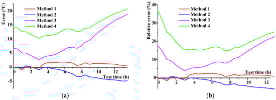
Figure 9.
Calculation error analysis of conductor-temperatures in Case 1: (a) error variation and (b) relative error variation.
From Figure 9, it can be seen that the errors of Method 1 were much less than those of others. Method 2 generally exhibited both a larger, negative error and relative error that increased with time and could reach −5.0 °C and −7%, respectively. The errors of Methods 3 and 4 were much larger than those of Methods 1 and 2, with a tendency to decrease at first and then increase. The initial errors caused by the solar radiation of Methods 3 and 4 were 6.7 °C and 14.1 °C, respectively. As time went by, the error kept decreasing until it reached the minimum value at hour 3, and then began increasing over time.
The average values of the absolute error and the relative error from the four methods were chosen to survey the difference under different laying conditions, which is illustrated in Figure 10.
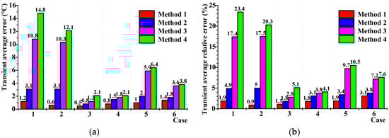
Figure 10.
Calculation errors of transient conductor-temperatures based on different radial position temperatures: (a) average errors and (b) average relative errors.
From Figure 10, we note the following:
- (1)
- Under all of the laying environments, Method 1 always exhibited minimal error and relative error that were less than 1.4 °C and 3.1%, respectively. This proved that the highest accuracy could be achieved when using the temperature of the insulation shield as the boundary condition. The errors and relative errors of Methods 2, 3, and 4 increased gradually, and the latter two methods exhibited similar errors.
- (2)
- When the cable was laid in the duct, Cases 1 and 2, the errors of Methods 3 and 4 were too large, while those of Methods 1 and 2 were smaller. When the cable was laid in water or backfilled soil, Cases 3–6, the limits of the errors caused by Methods 1 and 2 had little difference, but those caused by Methods 3 and 4 exhibited significant nonconformity, and the maximum was found in Method 4, at 1300 A loaded under the condition of water.
In this paper, the steady state of the conductor temperature was defined as that the range of conductor-temperature variation within 3 h was less than ±1 °C, so the mean value served as the steady temperature. As seen in Figure 11, the calculations based on Method 1 always exhibited a minimal steady error under all the laying conditions. The steady error and relative error were less than 1.7 °C and 2.6%, respectively. This proved that the best accuracy for the calculation of steady conductor temperature could be achieved when it was inverted from the temperature of the insulation shield. Method 2 had the better accuracy, with an error and relative error of less than 3.5 °C and 4.7%, respectively, while both errors for Methods 3 and 4 were much more. The steady errors and relative errors of the latter two methods were correlated with current density.
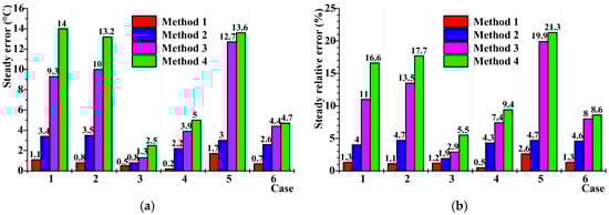
Figure 11.
Calculation errors of steady conductor-temperatures based on different radial position temperatures: (a) errors and (b) relative errors.
4.2. FEM Simulation Results of the Conductor Temperature
To examine the effectiveness of conductor temperature calculations, simulation models based on flow characteristics of the air gap between the waterproof compound and the aluminum were built up. The FEM simulation results of the cable’s thermal field in Case 1 are shown in Figure 12.

Figure 12.
Steady temperature distributions by FEM simulations based on Method 4 for Case 1: (a) Approach 1 and (b) Approach 2.
Both the tested and the simulation values of the steady conductor temperature in each case are presented in Table 4. In Figure 12 and Table 4, Approach 1 represents the convective flow of the air directly, while Approach 2 gives a combination of equivalent thermal resistivity and heat capacity for dissipation of the air between the waterproof compound and aluminum sheath. Boundaries 1, 2, 3, and 4 represent the insulation-shield, the center of waterproof compound, the aluminum sheath, and the jacket surface, respectively.
Table 4.
Steady conductor temperatures obtained by FEM simulations (°C).
When the effect of the convection and radiation, i.e., Approach 1, was considered, the simulation results were much close to the experimental results. However, when a combination of thermal resistivity and heat capacity to describe the heat transfer character of the air, i.e., Approach 2, was considered, the difference between the simulation and the experiment results was significant, which appeared similar calculation errors to that between the thermal circuit calculation and the experiment results in Figure 11. As for the air layer, convection and radiation are the primary heat dissipation ways, while the heat conductivity coefficient is very small; for instance, 0.0259 W/(K·m) at 20 °C. An appropriate correlation of the thermal resistance should be considered when Formula (1) was applied to the calculation of thermal resistance for the air layer.
5. Discussions
Both the thermal circuit calculation and the FEM simulation results indicated that the farther the temperature sensor was from the conductor, the more significant the error of the conductor-temperature calculation was. So, the factors influencing the conductor-temperature calculation errors were discussed below.
5.1. Effect of the Initial Temperature Difference on Errors
In Formula (6), the initial condition of each layer in the cable was assumed to be isothermal; however, the experimental conditions were different from this hypothesis. In particular, in Case 1, as shown in Figure 7a, the initial temperatures of the jacket surface and the aluminum sheath were obviously higher than those of other three structures, the latter was of similar temperature. This caused remarkably larger initial errors that were based on Method 3 or Method 4 than those Methods 1 and 2, demonstrating in Figure 9a. The influence of the obvious initial temperature difference ΔT0 between the conductor and the boundary of the second-order resistance-capacitance circuit shown in Figure 3 on the conductor temperature would decrease over time and the calculation errors would reduce. It also explained why the errors based on Methods 3 and 4 showed a decreasing tendency at the first several hours, and then increasing under the condition of the duct. When the cable was laid in water or backfilled soil, the temperature risings of the jacket surface and the aluminum sheath were gentle, so the influence of initial temperature on the calculation results was not significant. In these cases, the errors were mainly caused by the thermal resistivity inaccuracy. Placing the temperature sensor closer to the conductor, i.e., the insulation-shield and waterproof compound, would contribute to eliminating the effect of the non-isothermal initial temperature due to the environment.
5.2. Effect of the Thermal Resistivity on Errors
In this paper, the thermal resistivity from IEC standards, together with the parameters of quiescent air, were used in thermal circuit calculation. However, these values might be different from those calculated based on the measured temperatures. As is illustrated in Figure 8, this difference made the temperature-calculation results higher or lower than the measurements overall. So, we used the steady-state temperatures of the tested cable shown in Table 5 to calculate the thermal resistivities. The steady thermal circuit in Figure 2 ensures that the heat storage of the thermal capacitances kept constant in the steady state, so the thermal capacitances were regarded as open-circuit type. The mean values of the calculated thermal resistivity are given in Table 6.
Table 5.
Steady-state temperatures of the tested cables (°C).
Table 6.
Thermal resistivities of the tested 110 kV single-core XLPE cable [(K·m/W)].
As for the XLPE insulation, including the merged conductor shield and insulation shield, both the recommended and the calculated values were 3.5 (K·m)/W, which proved that the evaluation of the thermal resistivity of the insulation layer was precise. Homoplastically, for the thermal resistivity of the jacket, the recommended value was 3.5 (K·m)/W, while the calculated value was 3.3 (K·m)/W. To determine the influence of the thermal resistivity of the jacket, taking Case 1 as an example, the temperature of the aluminum sheath, θal, was inverted from the temperature of the jacket surface based on the thermal circuit of Method 4, and a comparison of the calculated values was then made with those measured. Figure 13 shows that the effect of the initial temperature decreased over time, and the calculation results of the aluminum sheath temperature was really close to those that were measured after 5.5 h. This means that the thermal resistivity of the jacket was acceptable, so in Figure 9, the error curves based on Methods 3 and 4 exhibited a trend of moving toward each other.
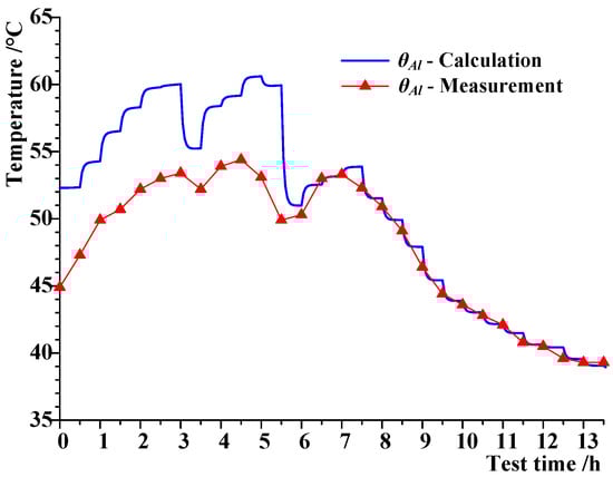
Figure 13.
Aluminum-sheath temperature calculation results (Case 1).
It seems that the recommended thermal resistivities for the dense and solid materials, i.e., the XLPE insulation and jacket, were consistent with the calculated based on measured temperatures, while the others not. For the thermal resistivity of the waterproof compound, the IEC recommended value was 6 (K·m)/W, which was less than the calculated value of 12.1 (K·m)/W in this paper. It should be noted that the negative error in Method 2 increased after hour 2. Since only part of the thermal resistivity of the waterproof compound was involved due to the temperature sensor placed in the center of the waterproof compound, the errors of Method 2 were not so remarkable, even though the calculated thermal resistivity of the waterproof compound was twice that of the recommended.
As for the air gap between the waterproof compound and sheath, the recommended thermal resistivity was 34 (K·m)/W, which is almost three times the calculated value of 12.1 (K·m)/W. An overlarge recommended thermal resistivity of the air gap was the dominant reason for the significant calculation errors found in Methods 3 and 4, which would increase with increasing current.
Based on the calculated values of thermal resistivity, calculation errors of the transient and steady conductor-temperature for the four methods in each case were recounted, and then illustrated in Figure 14.
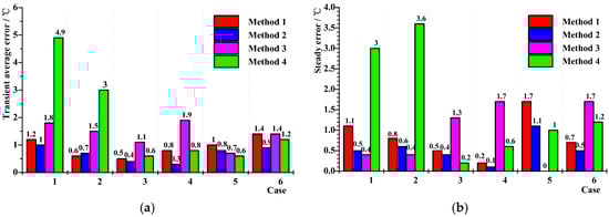
Figure 14.
Conductor temperature errors using tested thermal resistances: (a) transient and (b) steady.
For Method 1, the calculated insulation thermal resistivity was the same as the recommended, so the calculation errors were still small. Both the average errors and relative errors of Methods 2–4 in Figure 14 sharply decreased to a very low level when compared to the results using the recommended thermal resistivity shown in Figure 10 and Figure 11. Their errors of transient and steady conductor temperature were less than 1.9 °C and 1.7 °C, respectively, apart from the higher values that were found in the first two cases with the initial-temperature differences caused by solar radiation.
The simulation results of the steady conductor temperature were also updated when using the calculated thermal resistance to describe the heat transfer of the air, i.e., Approach 2. The result is illustrated in Table 7.
Table 7.
Simulation errors of the steady conductor temperatures by FEM simulation using the calculated thermal resistances (°C).
The simulation errors were less than 2.8 °C, apart from a higher value, 4.92 °C for Boundary 4 in Case 5. So, using the calculated thermal resistance, the FEM simulation results of Approach 2 were close to that of Method 1 as well as the measured results.
In summary, the thermal resistance of the air layer is the source of the largest error, so it seems that the temperature sensor should be placed closer to the conductor. Though the insulation-shield was the closest position to the conductor in this paper and led to the best accuracy, placing a temperature sensor in this position would have a potential risk of the direct contact with the insulation material. So, the waterproof compound was recommended for the better accuracy and good insulation security because the sensor was isolated from the insulation. Both the calculation and FEM simulation proved that when the uncertainty of thermal resistances, especially the air resistance was eliminated, the conductor temperature calculations using the temperatures of the waterproof compound or the aluminum sheath could obtain a close accuracy to that of insulation shield. The waterproof compound and the aluminum sheath, especially the latter, are more practical for engineering.
5.3. Effect of the Air Thermal Capacitance on Errors
From the point of dynamic response, the time constant of the circuit depends on its resistance and capacitance parameters. As shown in Figure 14a, when thermal resistivities were calculated, the calculation errors of transient conductor temperature would not beyond 1.9 °C, apart from two higher values found in Method 4. So, the thermal capacitances were generally valid because the calculation accuracy was high enough. Since the IEC standard has provided the volumetric specific heat of solid material, we only analyzed the variation of the air thermal capacitance in this paper.
For an actual air layer, both the density and specific heat are temperature-varying. For example, they are 1.205 kg/m3 and 1.005 kJ/(kg·K) at 20 °C, respectively, while 1.029 kg/m3 and 1.009 kJ/(kg·K) at 70 °C. When taking the temperature-varying thermal capacitance into account, the calculation errors of transient conductor temperature were updated using Boundaries 3 and 4 by FEM. The results are presented in Table 8.
Table 8.
Calculation errors of transient conductor-temperature using constant and temperature-varying thermal capacitances (°C).
In Table 8, the results of using the constant and the temperature-varying air thermal capacitance were almost identical. The effect of the temperature-varying thermal capacitance of the air was so insignificant within the range of cable’s temperature variation that the errors caused by it could be neglected. Thus, defining the air thermal capacitance as a constant is appropriate. In other words, it is the thermal resistance, rather than the thermal capacitances, which is the main error source of temperature calculation.
6. Conclusions
Four conductor-temperature calculation methods based on the temperature measurements of different radial positions in the cable were proposed, respectively, and were compared with the FEM simulations.
The results showed that the calculated conductor temperature based on the temperature of the insulation shield was closest to the measured, and that of the center of the waterproof compound was the closer. However, there was a remarkable difference between the measured and calculated results based on the temperature of the jacket surface or aluminum sheath. The results of FEM simulation agreed with those of the calculations.
The uncertainty of the thermal resistivities, especially that of the air between the waterproof compound and the sheath, is the main factor affecting the conductor-temperature calculations. Because of the differences in corrugation designs between manufacturers, it is difficult to recommend a constant for the thermal-resistance calculation of the air in standards. The influences of other factors are limited. The difference in the initial temperature of each radial position caused by the solar radiation mainly influenced the calculation based on the temperature of the jacket during the first several hours. In addition, the effect of the temperature-varying thermal capacitance of the air could be neglected.
To improve the accuracy of the conductor temperature calculation, the temperature sensor should be placed closer to the conductor. The waterproof compound was recommended for better accuracy and good insulation security. When eliminating the uncertainty of thermal resistances, especially the thermal resistance of the air between waterproof compound and aluminum sheath, the conductor temperature calculations using the temperature of the aluminum sheath could also obtain a high accuracy.
Acknowledgments
This work was supported by the Science and Technology Project of China Southern Power Grid (Grant No. K-KY2014-31).
Author Contributions
Lin Yang and Yanpeng Hao conceived and designed the experiments; Lin Yang, Weihao Qiu and Jichao Huang performed the experiments; Lin Yang, Weihao Qiu, Jichao Huang and Yanpeng Hao analyzed the data; Mingli Fu, Shuai Hou and Licheng Li contributed materials and analysis tools; Lin Yang, Weihao Qiu and Yanpeng Hao wrote the paper.
Conflicts of Interest
The authors declare no conflict of interest.
References
- Wang, Y.N.; Li, G.D.; Wu, J.D.; Yin, Y. Effect of temperature on space charge detrapping and periodic grounded dc tree in cross-linked polyethylene. IEEE Trans. Dielectr. Electr. Insul. 2017, 23, 3704–3711. [Google Scholar] [CrossRef]
- International Electrotechnical Commission. Calculation of the Current Rating, Parts 1 and 2, IEC Standard 60287-1 and IEC Standard 60287-2; International Electrotechnical Commission: Geneva, Switzerland, 2006. [Google Scholar]
- International Electrotechnical Commission. Calculation of the Cyclic and Emergency Current Rating of Cables—Part 2: Cyclic Rating Factor for Cables Greater than 18/30(36)kV and Emergency Ratings for Cables of All Voltages, IEC 60853-2; International Electrotechnical Commission: Geneva, Switzerland, 1989. [Google Scholar]
- Terracciano, M.; Purushothaman, S.; Leon, F.D.; Farahani, A.V. Thermal analysis of cables in unfilled troughs: Investigation of the IEC standard and a methodical approach for cable rating. IEEE Trans. Power Deliv. 2012, 27, 1423–1431. [Google Scholar] [CrossRef]
- Holyk, C.; Anders, G.J. Power cable rating calculations—A historical perspective. IEEE Ind. Appl. Mag. 2015, 21, 6–64. [Google Scholar] [CrossRef]
- Anders, G.J.; El-Kady, M.A. Transient ratings of buried power cables—Part 1: Historical perspective and mathematical mode. IEEE Trans. Power Deliv. 1992, 7, 1724–1734. [Google Scholar] [CrossRef]
- Al-Saud, M.S.; El-Kady, M.A.; Findlay, R.D. A new approach to underground cable performance assessment. Electr. Power Syst. Res. 2008, 78, 907–918. [Google Scholar] [CrossRef]
- Hwang, C.C.; Chang, J.; Chen, H.Y. Calculation of ampacities for cables in trays using finite elements. Electr. Power Syst. Res. 2000, 54, 75–81. [Google Scholar] [CrossRef]
- Nahman, J.; Tanaskovic, M. Calculation of the ampacity of high voltage cables by accounting for radiation and solar heating effects using FEM. Int. Trans. Electr. Energy Syst. 2013, 23, 301–314. [Google Scholar] [CrossRef]
- Gouda, O.E.; Dein, A.Z.E.; Amer, G.M. Effect of the Formation of the Dry Zone around Underground Power Cables on Their Ratings. IEEE Trans. Power Deliv. 2011, 26, 972–978. [Google Scholar] [CrossRef]
- Marshall, J.S.; Fuhrmann, A.P. Effect of rainfall transients on thermal and moisture exposure of underground electric cables. Int. J. Heat Mass Transf. 2015, 80, 660–672. [Google Scholar] [CrossRef]
- Gela, G.; Dai, J.J. Calculation of thermal fields of underground cables using the boundary element method. IEEE Trans. Power Deliv. 1988, 3, 1341–1347. [Google Scholar] [CrossRef]
- Millar, R.J.; Lehtonen, M. A robust framework for cable rating and temperature monitoring. IEEE Trans. Power Deliv. 2006, 21, 313–321. [Google Scholar] [CrossRef]
- Yilmaz, G.; Karlik, S.E. A distributed optical fiber sensor for temperature detection in power cables. Sens. Actuator A Phys. 2006, 125, 148–155. [Google Scholar] [CrossRef]
- Ukil, A.; Braendle, H.; Krippner, P. Distributed temperature sensing: Review of technology and applications. IEEE Sens. J. 2012, 12, 885–892. [Google Scholar] [CrossRef]
- Hao, Y.Q.; Cao, Y.L.; Ye, Q.; Cai, H.W.; Qu, R.H. On-line temperature monitoring in power transmission lines based on Brillouin optical time domain reflectometry. Optik 2015, 126, 2180–2183. [Google Scholar] [CrossRef]
- Zhao, L.J.; Li, Y.Q.; Xu, Z.N.; Yang, Z.; Lü, A.Q. On-line monitoring system of 110 kV submarine cable based on BOTDR. Sens. Actuator A Phys. 2014, 216, 28–35. [Google Scholar] [CrossRef]
- Cho, J.; Kim, J.H.; Lee, H.J.; Kim, J.Y.; Song, I.K.; Choi, J.H. Development and improvement of an intelligent cable monitoring system for underground distribution networks using distributed temperature sensing. Energies 2014, 7, 1076–1094. [Google Scholar] [CrossRef]
- Li, H.J. Estimation of soil thermal parameters from surface temperature of underground cables and prediction of cable rating. IEE Proc. Gener. Transm. Distrib. 2005, 152, 849–854. [Google Scholar] [CrossRef]
- Guo, J.J.; Zhang, L.; Xu, C.; Boggs, S.A. High Frequency Attenuation in Transmission Class Solid Dielectric Cable. IEEE Trans. Power Deliv. 2008, 23, 1713–1719. [Google Scholar]
- WG B1.35. A Guide for Rating Calculations of Insulated Cables, TB 640; International Council on Large Electric Systems: Paris, France, 2015. [Google Scholar]
- Tsili, M.A.; Amoiralis, E.I.; Kladas, A.G.; Souflaris, A.T. Hybrid Numerical-Analytical Technique for Power Transformer Thermal Modeling. IEEE Trans. Magn. 2009, 45, 1408–1411. [Google Scholar] [CrossRef]
- Van Wormer, F.C. An improved approximate technique for calculating cable temperature transients. IEEE Trans. Power Appl. Syst. 1955, 74, 277–281. [Google Scholar]
- Ruan, J.J.; Liu, C.; Huang, D.C.; Zhan, Q.H.; Tang, L.Z. Hot spot temperature inversion for the single-core power cable joint. Appl. Therm. Eng. 2016, 104, 146–152. [Google Scholar] [CrossRef]
- Zhao, J.K.; Fan, Y.B.; Wang, X.B.; Li, S.T.; Niu, H.Q. Thermal resistance properties of the part between metal sheath and conductor in high-voltage power cable. High Volt. Eng. 2008, 34, 2483–2487. (In Chinese) [Google Scholar]
- Power Cables with Cross-Linked Polyethylene Insulation and Their Accessories for Rated Voltage of 110kV (Um = 126kV)—Part 1: Test Methods and Requirements, Chinese Standard GB/T 11017.1; Standards Press of China: Beijing, China, 2014.
© 2018 by the authors. Licensee MDPI, Basel, Switzerland. This article is an open access article distributed under the terms and conditions of the Creative Commons Attribution (CC BY) license (http://creativecommons.org/licenses/by/4.0/).