Variance Characteristics of Tropical Radiosonde Winds Using a Vector-Tensor Method


1
Interdisciplinary Graduate School, Nanyang Technological University, Singapore 639798, Singapore
2
Energy Research Institute @ NTU, Nanyang Technological University, Singapore 637141, Singapore
3
UC, Singapore University of Social Sciences, Singapore 599491, Singapore
4
School of Mechanical and Aerospace Engineering, Nanyang Technological University, Singapore 639798, Singapore
*
Authors to whom correspondence should be addressed.
Energies 2018, 11(1), 137; https://doi.org/10.3390/en11010137
Submission received: 7 November 2017
/
Revised: 20 December 2017
/
Accepted: 22 December 2017
/
Published: 5 January 2018
(This article belongs to the Section L: Energy Sources)
Abstract
:In this paper, an exploratory study on the variance characteristics of upper-air winds in a near-equator monsoon region is presented. The data were obtained from historical radiosonde observations from up to 250 stations within the region of interest for the period between 1954 and 2013. An alternative method based on vector statistics was employed in this study which characterises the mean by a vector and the variance by a tensor. Unlike the conventional approach of using scalar wind speeds, this vector-tensor approach allows the directional properties of the variance to be studied. A suite of statistics to describe the geometric properties of the variance tensor was also developed. These characterise the size of the variance, its degree of anisotropy, and the alignment of the preferred direction (if anisotropy is present) with the direction of the mean wind vector. Through analysis of these statistics, several salient trends were observed for the middle troposphere. It was found that the variance size and anisotropy exhibit significant variation with height whereas the alignment with the mean vector varies with the mean wind magnitude instead. It was also found that the scalar variance increases with mean wind speed.
Keywords:
wind characteristics; variance; covariance matrix; random vector; radiosonde; monsoon; tropical; high-altitude1. Introduction
The statistical characterisation of the wind is an important step in the planning of major infrastructure projects. In the wind energy sector, such characterisation exercises, referred to as resource assessments, are carried out to assess the wind energy availability and predict prevailing wind patterns at potential sites for new wind power plants [1,2,3,4]. This is necessary for project financiers and operators to estimate the power output from the plant and hence calculate the potential returns from the investment. Wind farm designers also rely on this information to optimise the placement of individual wind turbines. In aviation, airport planners use wind information to place and orient runways. Airport runways are typically oriented along the direction of the prevailing wind to minimise crosswinds that can pose a hazard to flight safety. Poorly oriented runways with frequent strong crosswinds also increase the number of aborted landings and reduce the effective capacity of the airport [5]. While there are numerous studies on wind characteristics near the surface, such studies at higher altitudes are rare due to the lack of specific practical applications. However, with recent advances in high altitude wind power (HAWP) technologies [6], characterisation of higher-level winds could take on greater importance. In addition, it is a trivial fact in aviation operations that en-route winds are a major determinant of flight duration and fuel burn [7,8]. Comprehensive knowledge of these winds is thus important to construct better-optimised flight schedules, flight plans, and improve general operation efficiency.
Current methods of wind characterisation found in literature typically involve quantifying the statistics of the wind speed by its mean and variance values. Some studies take it a step further and fit the observed wind speed distribution to prescribed probability distribution functions, with the two-parameter Weibull distribution being the most commonly used [1,2,3,9,10,11]. More advanced methods may also include a spectral analysis to determine the frequencies of wind speed fluctuations [1,10]. When wind direction is concerned, the von Mises distribution is commonly used to describe the observed direction distribution [10]. In some cases, wind roses are used to provide a graphical representation of both the wind speed and direction on a single diagram [3,10,11]. While these methods are adequate for most practical applications, they consider the wind speed and direction as separate scalar quantities. This ignores the fact that wind measurements are actually vectors and that its speed and direction are two components of a single quantity. Even though the wind rose does provide an intuitive picture containing both the wind speed and direction, the representation is inherently graphical and difficult to manipulate mathematically. In this paper, the authors are proposing an alternative method to characterise the wind statistics that is based on the statistics of vectors. This method is similar to that employed by Koh and Ng [12] in their study on wind errors but is applied here directly onto actual wind measurements. The method is then used in an exploratory study of winds in the near-equator monsoon region using observation data obtained from radiosondes.
Radiosondes are instrument packages launched on weather balloons to collect atmospheric data as the balloon ascends through the atmosphere. They are a primary source of meteorological data, including horizontal wind speed and direction, for the upper atmosphere above the reach of ground-based measurement sensors. Unlike measurements by the ground-based sensors, radiosondes record data at various altitudes based on the pressure rather than at fixed physical heights above the ground. The World Meteorological Organisation (WMO) specifies eleven such pressure levels as mandatory for radiosonde observations. They are, from a lower to a higher level, 1000, 925, 850, 700, 500, 400, 300, 250, 200, 150, and 100 mb. The WMO also standardises two daily launch times at 00:00 and 12:00 UTC. Data from radiosondes are currently mostly used in operational weather forecasting where it serves as a source for data assimilation in numerical weather prediction (NWP) models [13]. Systematic studies on upper-air wind statistics using radiosonde data are rare, however, especially in the tropics. One such study was conducted by Koh et al. [14] where wind speeds in the equatorial monsoon region were investigated.
This paper seeks to accomplish two objectives. The first is to introduce readers to the alternative vector-based method for characterising wind statistics. This new method invokes the mathematics for describing random vectors, with particular focus on the variance which takes on the form of a tensor. The second objective is to present an exploratory study, performed both using the said method and the more conventional approach of using scalar wind speeds, to characterise the upper-air wind variance of the near-equator monsoon region using radiosonde data. The paper is structured as follows: the next section describes the proposed vector-based method and lists the wind statistics used in the subsequent radiosonde study. Section 3 gives an overview of the data source and the steps taken to process the data. Section 4 then provides the results, analysis of the results, and discussion. Section 5 derives the relation between the variance tensor and eddy diffusivity. Finally, Section 6 concludes the paper and Section 7 provides some suggestions for future studies.
2. Method
2.1. Mean Vector and Variance Tensor
Consider a set of n measurements of horizontal wind velocity v1, v2, v3, …, vn with corresponding magnitudes v1, v2, v3, …, vn. Each measurement is a two-dimensional vector with components vx and vy in the Cartesian x and y direction respectively. The statistics of the scalar wind speed can be characterised by its mean and variance as given by the following well-established equations:
In the proposed vector-based method, however, the characterisation of the whole velocity vector is sought. The mean and variance in this case, taking the form of a vector and a tensor respectively, are given by these equations:
Five independent terms, two from the mean vector and three from the variance tensor, are required to characterise the wind velocity as compared to only two for the wind speed. These additional terms capture the information on direction contained in the velocity vector and characterises the measured wind more holistically. Note that the variance tensor is also referred to as the covariance matrix in some texts.
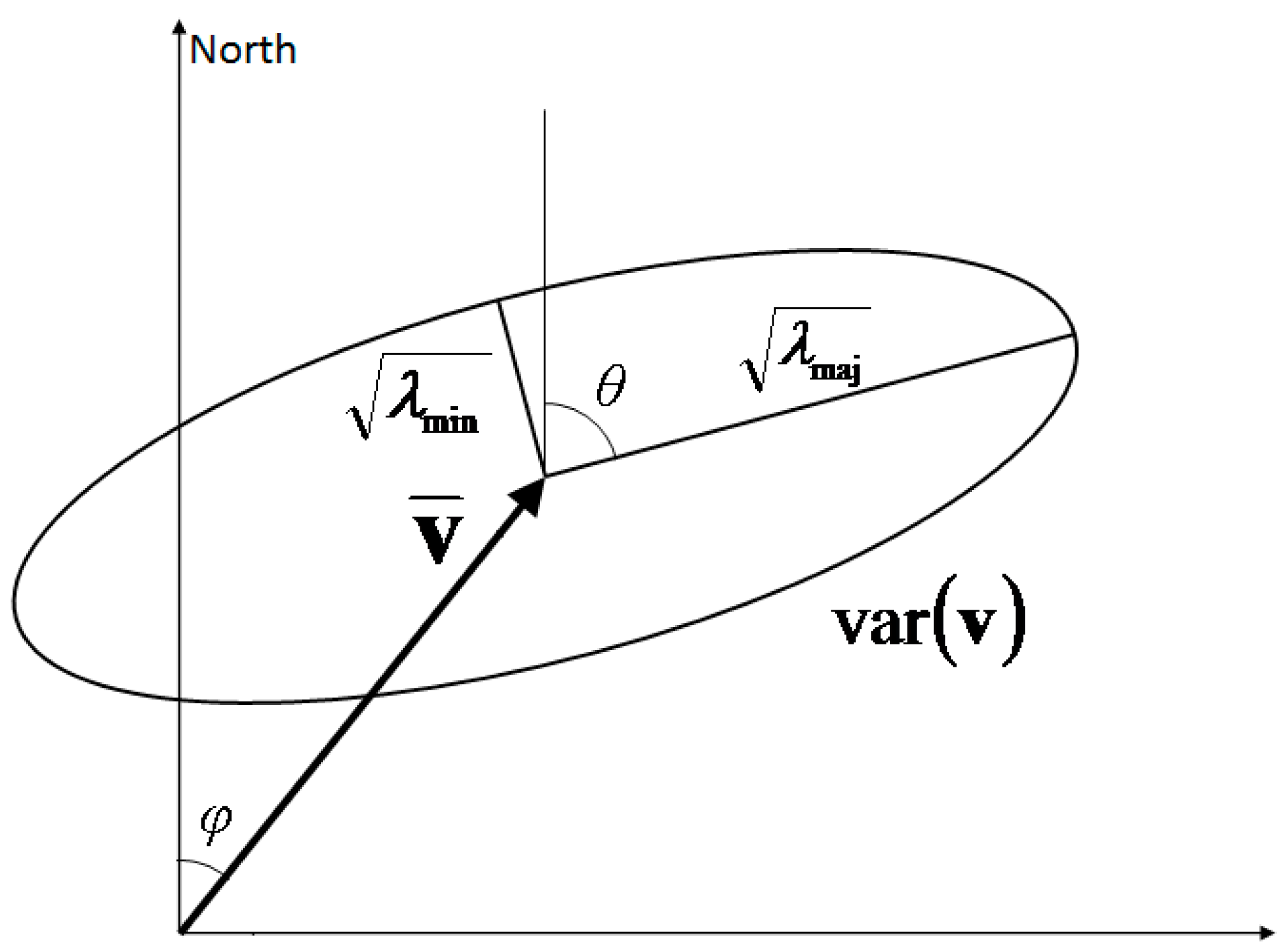
Visualising the geometry of the mean vector is simple. Its two independent terms can either be the two components of the vector, as in Equation (3), or be stated as its magnitude and direction. Visualising the variance tensor, however, is more abstract. Koh and Ng [12] described such a tensor graphically by means of an ellipse. In their approach, the eigenvalues, λmin and λmaj, and eigenvectors of the tensor matrix are first calculated. An ellipse can then be constructed with the square-root of the eigenvalues being the lengths of the semiaxes, and the said semiaxes being oriented in the direction of the corresponding eigenvectors. When the centre of this ellipse is plotted on the point representing the mean vector on a 2D Cartesian plane, the perimeter of the ellipse would represent the boundary of one standard deviation away from the mean. An explanatory figure is provided as Figure 1 for clarity.
Interested readers are referred to Koh and Ng [12] for more elaboration. One important feature of this ellipse representation, henceforth referred to as the variance ellipse, is the identification of the principal axes of the variance tensor. For a two-dimensional horizontal wind, the principal axes, which are the semiaxes of the variance ellipse, are axis of the maximum and minimum variance
2.2. List of Statistics Used in This Study
The following is the list of the statistics and their associated symbols used in the subsequent wind characterisation study. They can be divided into scalar-based and vector-based statistics. The vector-based statistics are specifically designed in this study to describe the geometric properties of the mean vector and variance tensor as described in the previous subsection.
2.2.1. Scalar-Based Statistics
- Mean wind speed, : Mean of the wind speed. This is given by Equation (1).
- Scalar variance, : Variance of the wind speed. This is given by Equation (2).
2.2.2. Vector-Based Statistics
- Magnitude of mean velocity, Vt: Magnitude of the mean vector. This is given by:
- Direction of mean velocity, ϕ: Direction bearing of the mean vector. 0° ≤ ϕ < 360°, measured clockwise from the cardinal north.
- Trace of the variance tensor, σ2t: This measures the general size of the variance and can be considered analogous to the scalar variance. It is given by Equation (6). The two expressions given in Equation (6) are equivalent because the trace is an invariant of a tensor. In fact, σt is properly the standard deviation of the wind vector and is depicted by the size of the ellipse in Figure 1. (Note that 4σt is the perimeter of the rhombus formed by joining the tips of the semiaxes of the ellipse in Figure 1.)
- Eccentricity of the variance tensor, ε: This measures the degree of anisotropy in the variance. Bounded from 0 to 1, ε = 0 indicates equal variance in all directions (variance ellipse is actually a circle) whereas ε = 1 indicates variations only along a particular axis (semiminor axis of the ellipse has zero length). To be distinguished from the conventional definition of eccentricity in the geometry of conic sections, the definition of eccentricity used in this study follows the one proposed by Koh and Ng [12] and is more properly termed “symmetrised eccentricity, εs” by Koh, Wang and Bhatt [15] although in this paper we shall call it “eccentricity” for convenience. It is given by:
- Orientation of the variance tensor, θ: Direction bearing of the axis of maximum variance. This is a principal axis of the variance tensor and also the semimajor axis of the variance ellipse. Because this statistic measures an axis rather than a specific direction, its value is bounded within a half circle: 0° ≤ θ < 180°, measured clockwise from the cardinal north.
The three statistics, σt, ε, and θ, capture all information in the variance tensor which can be rewritten simply as in Equation (31) of Koh, Wang and Bhatt [15]:
where I is the identity tensor.
An additional statistic, η, is introduced that measures the alignment of the mean vector to the axis of maximum variance. It is defined as the absolute dot product of unit vectors in the direction of ϕ and θ. Mathematically, this can be expressed by:
where denotes a unit vector in the direction of the angle given by its subscript. The value of η is bounded from 0 to 1 with η = 1 indicating perfect alignment between the mean velocity and the axis of maximum variance. For the current study, η is investigated in lieu of ϕ and θ to explore an observed tendency for the two directions to align.
3. Data
3.1. Data Source
The radiosonde data used in this study was obtained from the Integrated Global Radiosonde Archive (IGRA). The archive contains records of meteorological data from radiosonde observations taken from upper-air observation stations throughout the world. One useful feature of the data is that it has undergone relevant quality-control (QC) procedures and can be considered free of erroneous readings and outliers [16]. IGRA is maintained by the United States National Oceanic and Atmospheric Administration (NOAA) and is accessible by the public at no cost.
For the current study, data from stations in a rectangular region bounded by 15° S and 15° N in latitude and 20° W and 155° E in longitude are considered. This represents a near-equator monsoon region which includes the entire longitudinal extent of the areas that experience the Asian and African monsoons. The region encompasses equatorial Africa and Indian Ocean, southern tip of the Indian subcontinent, and the Maritime Continent. There are a total of 250 stations within the selected region. Even though records for some stations in IGRA date as far back as 1946, a check revealed that many stations in the current region of interest only began regular observations in 1954. As such, this study only uses data taken from between 1954 and 2013. In addition, the study only considers data collected at the eleven WMO mandatory pressure levels and at the standard radiosonde launch times of 00:00 and 12:00 UTC.
3.2. Data Processing
The data for each station, at each pressure level, and for each launch time were processed individually. Individual measurements for wind velocity were grouped into sets with each set corresponding to a particular station, at a particular pressure level, and to a specific launch time. These sets were then further split into four each with each corresponding to one of the four monsoon or intermonsoon seasons commonly associated with the region. The result is 88 sets of raw observation data for each station in the selected geographic region, with each set of data taken to represent the wind behaviour at a particular combination of pressure level (×11), season (×4), and time (×2: 00:00 and 12:00 UTC). The four seasons mentioned are two monsoon seasons: June to September (JJAS) and December to March (DJFM), and two intermonsoon seasons: April to May (AM) and October to November (ON). In regions that experience monsoon wind patterns, the prevailing wind comes from opposite directions during the two monsoon seasons whereas winds are generally light and variable during the intermonsoon seasons.
In order to ensure the statistical significance of the computed statistics, sets containing too few observation data were discarded from the study. A minimum number of 600 individual measurements was enforced for sets representing the monsoon seasons JJAS and DJFM, and 300 individual measurements for sets representing intermonsoon seasons AM and ON. This is roughly equivalent to the amount of data collected in five years of continuous records. The list of statistics introduced in Section 2.2 were then computed for each of the remaining sets of data.
3.3. Tests of Significance
An additional layer of significance checks was carried out on the computed statistics to weed out those that do not make physical sense. Firstly, t tests were performed on each set of observations to identify those potentially characterised by a zero mean velocity. The tests were carried out on the wind components in the two cardinal directions separately and at a 95% confidence level (two-tailed) against the null hypotheses and . A set is deemed to be characterised by a zero mean velocity if the null hypothesis cannot be rejected in both directions. In such cases, the direction of the mean velocity ϕ would have little meaning and would therefore be discarded. Next, χ2 tests for variance were performed to identify sets characterised by a very small trace of the variance tensor σ2t. The tests, using a modified test statistic given by:
where n is the number of observations, σ20 is the hypothesised value of the trace, and 2(n − 1) is the degree of freedom of the χ2 distribution, were carried out at a 95% confidence level (one-tailed) against the null hypothesis σ2t < 0.01Vt2. A set is deemed to be characterised by a very small trace if the null hypothesis cannot be rejected and its tensor-linked statistics, eccentricity ε and orientation θ, would then be discarded. Even if the trace is not small, a F test for equality of variances would further be performed to determine if the variance tensor is isotropic by comparing the variance in the two principal directions. The F tests were carried out at a 95% confidence level (two-tailed) against the null hypothesis λmin = λmaj. A set is deemed to be characterised by an isotropic variance if the null hypothesis cannot be rejected. In such cases, the orientation of the variance tensor θ would make little sense and would be discarded. Finally, noting that the alignment statistic η is a dot product derived from ϕ and θ, η would also be discarded when either ϕ or θ was discarded. A description of these standard tests can be found in most texts on statistics and hypothesis testing such as [17]. A summary of the tests performed is given in Table 1.
4. Results
4.1. Qualitative Scatter Analysis
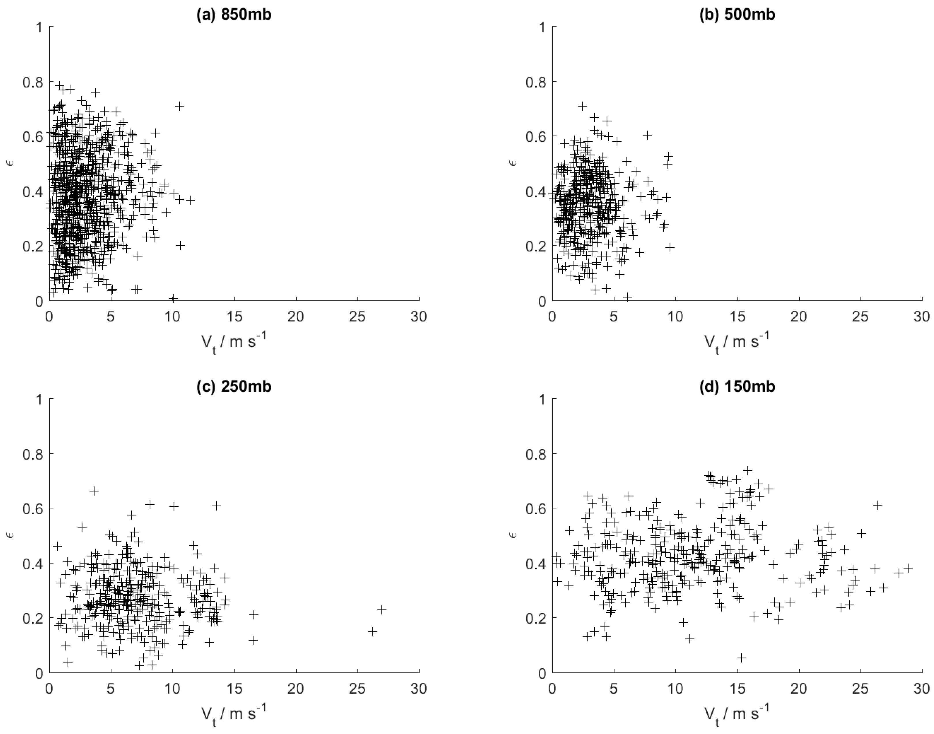
The characteristics of the computed statistics were visualised using scatter plots. Four scatter relations are considered: σ2s vs. Vs, σ2t vs. Vt, ε vs. Vt, and η vs. Vt. For each relation, eleven separate plots were made to describe the scatter at each of the eleven pressure levels considered. Four of these are representatively shown in Figure 2, Figure 3, Figure 4 and Figure 5: 850 mb (lower troposphere), 500 mb and 250 mb (middle troposphere), and 150 mb (upper troposphere). Each scatter point in these plots represents the statistics obtained for a single set of the observation data as described in the previous section. The sets can be of different seasons or launch times but all points on a single plot are from sets of the same pressure level.
A quick inspection of the scatter plots reveals some salient features. The plots of σ2s vs. Vs in Figure 2 show a trend of increasing σ2s with increasing Vs. This implies that the scalar variance tends to get larger with higher mean wind speed. Also, the spread of scatter points increases with increasing Vs, giving the impression that the scatter points are fanning out from the origin. This implies a greater variability of the scalar variance at higher mean wind speeds.
As for the plots of σ2t vs. Vt (Figure 3), which are the vector equivalent of σ2s vs. Vs, neither σ2t nor its spread seems to be related to Vt. However, the spread of σ2t exhibits a peculiar skewness with high density of scatter points coalescing towards a pseudo lower bound and the density gradually tapering off towards higher values of σ2t. It is noted that this pseudo lower bound appears to move upwards with a higher pressure level. This implies that the trace of the variance tensor tends to become larger with increasing height.
For the plots of ε vs. Vt in Figure 4, the spread of ε reduces and appears to tend towards a particular median value of ε as Vt increases. This implies that the degree of anisotropy in the variance tends towards a certain value at higher magnitudes of the mean wind velocity whereas at lower magnitudes, a greater variability of the anisotropy can be expected. It is also noted that the median ε value and the spread are different in each of the plots, suggesting that these characteristics are related to the pressure level. Finally, for the plots of η vs. Vt in Figure 5, the spread of η reduces and η tends sharply towards 1 with increasing Vt. Furthermore, even at low Vt, the spread of η is also highly skewed towards η = 1. This implies that the direction of the mean wind velocity tends to align with the axis of the maximal variance and especially so at higher magnitudes of mean wind velocity.
4.2. Regression Fitting of Percentile Lines
In furthering the analysis, percentile lines were used to quantify the observed scatter patterns. These percentile lines describe how the location and spread of the scatter points change with Vs or Vt, similar to how a standard regression line describe that for the scatter mean. Five percentiles were considered: 10th, 25th (1st quartile), 50th (median), 75th (3rd quartile), and 90th percentile. The percentile lines were obtained using a two-step process. The first involved binning of scatter points in each scatter plot into bins in the horizontal Vs or Vt-axis. For each of the five percentiles considered, a regression point was computed for each bin. The vertical coordinate of this point is the percentile calculated for only the scatter in the particular bin and the horizontal coordinate is the bin centre. In order to ensure statistical significance, regression points calculated from bins with less than five scatter points were discarded. The second step was to obtain the percentile line by fitting a regression line through the regression points from all the bins. For this, a weighted linear least-squares regression analysis was used with the regression points weighted by the number of scatter points in the respective bins. Two binning schemes were tested in the analysis. A coarser scheme has, for all pressure levels except 150 mb, a bin width of 2 m·s−1 for Vs or Vt between 0 and 20 m·s−1 followed by a single bin from 20 to 30 m·s−1. For the 150 mb pressure level, the scheme has a bin width of 2 m·s−1 between 0 and 24 m·s−1 followed by a single bin from 24 to 30 m·s−1. An inspection of the scatter points showed none of them falling beyond 30 m·s−1. The finer bin scheme contains smaller bin widths and twice the number of total bins. It has, for all pressure levels other than 150 mb, a bin width of 1 m·s−1 for Vs or Vt between 0 and 20 m·s−1 followed by two larger bins from 20 to 25 m·s−1 and 25 to 30 m·s−1. For the 150 mb pressure level, this scheme has a bin width of 1 m·s−1 between 0 and 25 m·s−1 followed by a single bin from 25 to 30 m·s−1. It was found that the use of either binning scheme did not alter the conclusions of the study. The results presented hereafter in this paper are that obtained for the finer scheme.
For the scatters of σ2s vs. Vs, σ2t vs. Vt, and ε vs. Vt, linear relations were assumed between percentiles of σ2s, σ2t, ε and Vs/Vt. The equations of the percentile lines fitted take the form:
In these equations, C, D, E, L, M, and N are fitting coefficients which characterise the percentile lines and that in turn characterise the scatters. Since five percentile lines were fitted for each scatter and eleven scatters, one for each pressure level, were made for each scatter relation, the fitting coefficients obtained can be functions of both the pressure level and the percentile. This is denoted by the subscript %|h: for example, L25%|500 would denote the L coefficient for the 25th percentile line of the 500 mb scatter. The same notation is also used to uniquely identify equations of individual percentile lines as shown by the left-hand-side terms of Equations (11)–(13). In the linear Equations (11)–(13), L, M, and N are coefficients of gradient and they give the correlation between the percentile and Vs/Vt. C, D, and E, on the other hand, are axis-intercept coefficients and they give the value of σ2s, σ2t, ε at each percentile when Vs/Vt approaches 0 m·s−1.
For the scatter relation η vs. Vt, however, the percentile lines that would describe the scatters are clearly not linear. An exponential relation, as given by the form:
is proposed instead. Linear fitting of the lines were performed in the logarithmic space using the linearised form of Equation (14) as shown by:
Here, B is the gradient coefficient which indicates how sharply the percentile line tends towards η = 1 whereas A is the intercept coefficient with 1 − A being the value of η at each percentile as Vt approaches 0 m·s−1. If A = 1 (ln A = 0), the percentile line passes through the origin.
4.3. Vertical Profiles of Fitting Coefficients
The results for the fitting coefficients L, M, N, C, D, E, A, and B are plotted in Figure 6, Figure 7, Figure 8, Figure 9, Figure 10, Figure 11, Figure 12 and Figure 13. As separate scatters were created for each individual pressure level, vertical profiles of the fitting coefficients could be obtained and plotted for each of the percentiles considered. In the plots, the pressure level is plotted on the horizontal axis from a lower level to a higher level while the value of the respective fitting coefficient is plotted on the vertical axis. The results obtained for the different percentiles are represented by markers of different colours. On top of the point-estimated values obtained from the regression analysis, the 98% confidence intervals for each estimate are also given as denoted by the co-located error bars.
In Figure 6, the point estimates for the coefficient L are positive at all pressure levels except 1000 mb and 925 mb. Even at these two levels, the confidence intervals obtained do not exclude the possibility of L being positive. Two further features were observed based on an impressionistic observation of the plot that also takes into account the error bars. First, the value of L at each pressure level appears to increase with higher percentiles.
This implies that the gradient of the percentile lines in the σ2s vs. Vs scatters increase with the percentile and this is consistent with the earlier qualitative observation that the scatter points appear to fan out from the origin. Next, it was also observed that the value of L for each percentile could be the same regardless of the pressure level. This possibly suggests a constant vertical profile.
In Figure 7, the point estimates for coefficient C are scattered about the C = 0 line. A similar impressionistic observation of the plot suggests that the value of C could be zero as many of the error bars do contain the zero line. This implies that the percentile lines in the σ2s vs. Vs scatters pass through the origin and this is again in line with the earlier qualitative observation.
For the gradient coefficients M and N in Figure 8 and Figure 10, respectively, the plots are similar to C in that the point estimates also scatter about zero and that many of the error bars contain the zero line. This implies that the scatters of σ2t and ε do not correlate significantly with Vt. Also, it was observed specifically in Figure 10 that the point estimates for N at the 1000 mb and 925 mb pressure levels are more negative as compared to the other pressure levels.
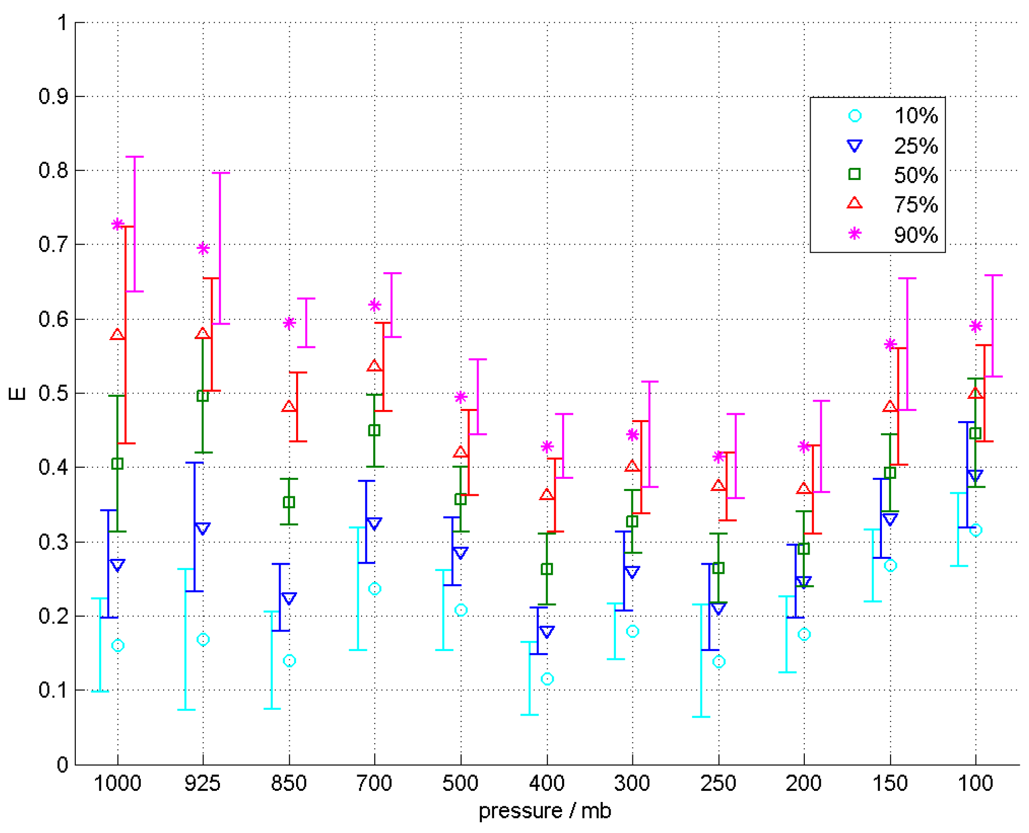
In Figure 9 and Figure 11, the plots of coefficients D and E show non-trivial vertical profiles with salient features. This is notable as unlike the other coefficients, the error bars here are generally smaller compared to the overall trends exhibited by the point estimates and this excludes the possibility of a constant vertical profile. The coefficient D in Figure 9 shows an increasing trend towards higher pressure levels while the coefficient E in Figure 11 shows a gradual decreasing trend up to about the 200 mb pressure level followed by a sharper increasing trend above it.
For the scatter relation η vs. Vt, it was observed in Figure 12 that the point-estimated values for ln A (and thus also for A) at each pressure level decrease with higher percentiles. This means that the η-axis intercept of the percentile lines, given by 1 − A, increase with the percentile. The observation is expected and in fact necessary for the percentile lines to stack in their proper order as Vt approaches 0 m·s−1.
One other feature, noted based on an impressionistic observation of Figure 12, is that the value of ln A for each percentile appears to be the same regardless of the pressure level. This implies that the η-axis intercept of each percentile is the same for all pressure levels. Finally, in Figure 13, an impressionistic observation of the plot suggests that coefficient B could be a non-zero constant with a same value regardless of the percentile or pressure level. This, together with the observations made of A, would imply that the scatters of η vs. Vt are characteristically similar for all the pressure levels.
4.4. Simplifying Relations for L, M, N, C, A, and B.
Using the impressionistic observations described above, the following simplifying relations for the fitting coefficients L, M, N, C, A, and B are hypothesised. No such hypothesis was made for the coefficients D and E. In the Equations (16) and (20) below, the dropping of h in the subscript of the right-hand-side terms is to denote that the coefficient is hypothesised to not depend on the pressure level but is still dependent on the percentile.
To examine the validity of the hypothesised relations, the following test was carried out. Consider a single result of a fitting coefficient. Assuming the hypothesised value to be true, the probability of the 100p% confidence interval (p = 0.98 in the plots shown above) not including the hypothesised value is 1 − p. Now, further consider the 55 instances of results, corresponding to the five considered percentiles and the eleven pressure levels, for each fitting coefficient. The probability that k or more of them do not include the hypothesised value can be modelled by the binomial distribution and is given by:
where K is the random variable denoting the number of confidence intervals not including the hypothesised value and n is the total number of instances of results (n = 55 in this case). Using this logic, if the value of k observed from the results is such that the probability p(K ≥ k) is less than the significance value 1 − p, it can be concluded that there is sufficient evidence that the hypothesised value is not correct. Otherwise, even though rigourous statistical theory would say no conclusions can be made, for the purpose of this work it is taken that the hypothesised value is sound. Note that the hypothesised values for coefficients L, A, and B are not explicit. For these cases, k was obtained by selecting a hypothesised value for the coefficient that minimises k.
Table 2 shows the results for k for the six fitting coefficients with hypothesised relations. Also given is the value of kcrit, the critical value of k such that the hypothesised relation is rejected if k ≥ kcrit. The results show that the hypothesised relations for coefficients L, M, C, and B are not supported. On closer investigation, however, it was realised that most instances with non-conforming confidence intervals are for either the higher levels at or above 150 mb, levels near the tropopause, or the lower levels at or below 850 mb, levels within the surface boundary layer or affected by topography. Removing these levels, Table 3 shows the results for k considering only the mid-tropospheric levels of 700 mb to 200 mb (with consequent reduction of n from 55 to 30). These new results show that the hypothesised relations for all the coefficients are sound when considering only the middle troposphere.
4.5. Implications and Discussion
Assuming the proposed relations given in Equations (16)–(21) are correct, some inferences can be made regarding the characteristics of σ2s with respect to Vs and σ2t, ε, and η with respect to Vt. Equations (23)–(26) in the following paragraphs show Equations (11)–(14) rewritten to reflect the simplified relations.
For σ2s, the coefficient L says that the percentile lines at each percentile have positive gradients and are the same for all pressure levels. Furthermore, the coefficient C suggests that all these lines pass through the origin. This implies two things. First, the scalar variance can be expected to increase with the mean wind speed and notably, for the inference to make physical sense, zero variance is expected for a no wind condition (i.e., zero mean wind speed, noting that wind speed is always positive or zero). Second, the scatters of σ2s vs. Vs are characteristically similar for all pressure levels. This implies that the scalar variance, while dependent on the wind speed, does not depend on the pressure level.
The characteristics of σ2t is, in contrast, quite the opposite. The coefficient M taking zero value implies that the trace of the variance does not depend on the magnitude of the mean wind. Also, the coefficient D shows a clear vertical profile in Figure 9 that indicates dependence on the pressure level. Since M = 0, D, rather than only being an intercept value, can be regarded as indicative of the value of σ2t at each percentile regardless of Vt. The vertical profile of D observed is such that it implies the standard deviation (the size of the ellipse in Figure 1) grows larger with height until near the tropopause level. This trend could easily be mistaken for an increasing trend with the wind magnitude as the magnitude of the mean wind velocity too increases with height. However, the scatter analysis showed that the dependency is on the pressure level and not the wind velocity.
ε shows similar characteristics to σ2t in that it does not depend on the magnitude of the mean wind but is dependent on the pressure level. The vertical profile of E in Figure 11 shows that the spread of the eccentricity reduces with height as the higher percentile lines approach the lower percentile lines which remain around the same value up to about the 200 mb pressure level. In this sense, the wind variance gets more isotropic with height. But upon nearing the tropopause (at pressures lower than 200 mb), the eccentricity seems to rise while keeping the same spread, denoting increasing anisotropy in the wind variance.
For η, Equations (20) and (21) for coefficients A and B further the description of η by saying that the scatters of η vs. Vt are characteristically identical for all pressure levels. Moreover, the constant value of B across percentile lines lends fundamental support that the spread of η tightens as the mean wind gets stronger and implies a growing tendency for the largest variance to occur in the direction of the mean wind as the mean wind strengthens. This last point is not a logical necessity but seems to be an interesting result of fundamental wind dynamics.
Table 4 and Figure 14 summarise the characteristics of σ2s, σ2t, ε, and η on their dependencies on Vs, Vt, and pressure level.
The increase of the scalar variance with mean wind speed can be explained by the other three results in Table 4. Appendix A proves the following identity:
which implies, using the result in Table 4 that σ2t is independent of Vt:
Thus, σ2s increases with Vs (d(σ2s)/d(V2s) > 0) if and only if V2s increases more slowly than V2t (d(V2s)/d(V2t) < 1) as the mean wind strengthens (Vt increases). Appendix B proves that this is indeed so for the case of small variations compared to the mean wind. Here, we offer a consistent, heuristic explanation for the general case. As the mean wind gets stronger, the size and anisotropy of the wind variations (σ2t and ε) remain constant but there is greater alignment of the direction of wind variations with the direction of the mean wind, as Table 4 says. Such alignment leads to more effective variation in the magnitude of the wind vector and so σ2s increases. With the constraint set by the identity in equation (27), V2s must increase more slowly than V2t, or otherwise, decrease. The latter case of decreasing V2s occurs when there are frequent, large enough variations compared to the mean wind speed: from Equation (28), negative d(V2s)/d(V2t) implies that d(σ2s)/d(V2s) = (σs/Vs) dσs/dVs < −1 and so σs/Vs > |dVs/dσs|. However, our result in Table 4 that σ2s increases with Vs and hence V2s is explained by the former case, where the wind variations are sufficiently small most of the time, i.e., qualitatively more like the case proven in Appendix B.
Some caveats are to be noted when considering the trends inferred above. Firstly, the proposed simplifying relations were shown to be valid only for the mid-troposphere between the 700 mb and 200 mb pressure levels. This means that the trends described are strictly valid only within this same part of the atmosphere. While no specific physical mechanisms will be proposed in this paper to explain the discrepancy at the lower and the higher levels, these excluded levels represent two unique parts of the troposphere. The lower levels at 850 mb and below is within the planetary boundary layer and are affected by the mountainous terrain found in parts of the monsoonal tropics (e.g., Sumatra, Borneo, East Africa). The obstructions caused by topography as well as friction against the planetary surface can cause distortions to wind flow. Similarly, at the higher levels of 150 mb and 100 mb pressure, distortions to the flow dynamics may also happen due to outflow from deep convection near the tropopause. The second caveat is that the results are applicable only within the specified near-equatorial monsoon region for which the radiosonde data for this study have been obtained. As scatter plots were used to derive the trends and implications, the inferred trends can only be considered as an aggregate for the entire geographic region being studied and that the trends observed at specific individual locations may be considerably different.
5. Relation between Wind Variance and Eddy Diffusivity
Consider the momentum equations (i.e., Navier-Stokes equations) for the atmosphere written with pressure as the vertical coordinate. At synoptic scales, the atmosphere can be approximated to be in hydrostatic balance and vertical advection terms are thus dropped. The resulting equations are in the form used in quasi-geostrophic approximation [18] and are given by:
where ψ is the geopotential, the horizontal wind v has been approximated by the (non-divergent) geostrophic wind vg, Dg/Dt represents the material derivative following the geostrophic motion, and F denotes body forces per unit mass including the Coriolis force. Noting that at planetary scales over climatological time-scale, vg can be thought of as a stochastic vector, we apply Reynolds averaging and considering only the resultant covariance terms, we obtain:
where X = var(v) is introduced to simplify the notations. Equation (30) is identical to the Reynolds-averaged Navier-Stokes equations with the exception that partial derivatives are evaluated holding the pressure constant instead of vertical height. The right-hand-side term of the equation accounts for the contributions to the total acceleration of the mean wind due to the stochastic fluctuations of the wind vector.
We now rewrite the covariance terms using the framework below:
where J is a matrix of coefficients and is the deformation rate of the mean geostrophic flow. We define the diffusivity matrix as the symmetric part of J:
K is responsible for the diffusion of momentum by eddy motion. Thus, combining Equations (31) and (32) and assuming is invertible, we obtain in Equation (33) the relation between the eddy diffusivity tensor and the velocity variance tensor:
One example when is invertible is when the mean flow is irrotational and the deformation rate is simply the (non-vanishing) strain rate of the mean geostrophic flow. In this case, the diffusivity tensor KS and the eddy diffusive flux XS are:
The eddy diffusive flux XS is the contribution to the overall velocity covariance (i.e., the momentum flux) due to the diffusion of momentum by eddies.
The significance of Equations (33) and (35) is that from the velocity covariance and mean flow, it is possible to diagnose the eddy diffusivity and this may aid the prognostic modelling of the mean flow over long time-scales or the theoretical understanding of the eddy momentum transport in the atmosphere.
6. Conclusions
In this paper, an alternative method was proposed for the statistical analysis and qualitative characterisation of atmospheric winds. This method is based on the statistics of vectors and features additional terms, in the form of a vector for the mean and a tensor for the variance, to more holistically describe the wind statistics. Several statistical measures based on the geometric interpretation of the variance tensor were also designed in this study. They are namely the trace of the variance tensor (the square-root of which is the standard deviation of the vector wind), the symmetrised eccentricity, and also the alignment measure η. Unlike the more traditional scalar analysis, these statistical measures, each with its own physical interpretation, allow the directional properties of the variance to be captured and analysed. The above methods were applied in an exploratory study of radiosonde wind data from a near-equator monsoon region. Through the use of scatter analysis, several trends were identified:
- (1)
- The scalar variance increases with the mean wind speed but is not affected by the pressure level;
- (2)
- The standard deviation and the anisotropy of the wind variations (measured by σt and ε) are not dependent on the magnitude of the mean wind vector (Vt) but show clear dependence on the pressure level;
- (3)
- The axis of maximal variance tends to align with the direction of the mean wind at stronger mean wind velocity but this behaviour is not affected by the pressure level.
Vector-based statistics, being more comprehensive summarising wind variance information, can provide insight into the scalar-based statistics. In particular, increasing alignment of maximal wind variations in the direction of the mean wind vector provides an explanation for the observed increase in scalar variance with mean wind speed.
It was also noted that the trends observed in this study appear valid only for the middle troposphere. While the study is primarily statistical in nature and no physical explanations were given for the observed trends, or lack thereof, some speculations were made with regards to the lower and the upper parts of the troposphere. Nevertheless, the results of this work can serve as a basis for future investigations into the physical mechanisms behind the observed trends and the discrepancy in the lower and upper troposphere. It is also hoped that this work would spark further interest in the use of vector-based approaches in the statistical characterisation of winds.
7. Suggestions for Future Studies
The work presented in this paper provided characterisation of radiosonde wind data using the well-established statistical concepts of mean and variance, albeit in a vector-tensor formulation. Other more sophisticated methods of analysing such data exist that may also yield further insights into the behaviour of upper-air winds in the monsoonal tropics. For example, artificial intelligence and machine-learning based methods on pattern recognition or trend prediction [19,20] can identify features within the data time series that are not captured by the mean and variance. On the point of time series analysis of stochastic vectors, methods exist by which the time evolution of a random vector can be described. Vasconcelos et al. [21] expanded upon such a method in which the diffusion matrix of the multivariate Fokker-Planck Equation undergoes an eigensystem analysis similar to what was done to the variance tensor in this paper. While prediction of time series is not an objective of this paper, it is definitely something also of interest to users of wind information in the light of the relation between the eddy diffusivity and the variance tensor of the flow derived in Section 5.
Acknowledgments
This research was supported by Energy Research Institute @ NTU through the research grant of Economic Development Board of Singapore (EIRP grant NRF2013EWT-EIRP003-032).
Author Contributions
Tieh-Yong Koh conceived the original idea for the study and directed a major part of the analysis when he was at Nanyang Technological University. He also explained the relationship between the scalar variance and the mean wind speed and provided the relevant proofs in Appendix A and Appendix B. Jing-Jin Tieo carried out the analysis and wrote the paper. Both Martin Skote and Narasimalu Srikanth gave important suggestions on various aspects of the work (method, analysis, context, etc.). Martin Skote also revised the drafts of the manuscript.
Conflicts of Interest
The authors declare no conflict of interest.
Appendix A
Consider a random wind vector v with mean component and fluctuating component v’. For simplicity of notation, the y-direction is defined to be in the direction of . Thus, the components of in the x and y directions are 0 and Vt respectively. The x and y components of v’ are denoted as vx’ and vy’. By definition:
Therefore,
using Equation (6) and noting that as the mean of fluctuating components is by definition zero.
Also, consider the magnitude of v as the scalar wind speed. We can write:
where |v|’ denotes the fluctuating component of the wind speed. Therefore,
Combining Equations (A2) and (A3), the identity given by Equation (27) is thus proven.
Appendix B
For small variances, applying Taylor series expansion on Equation (A1) up to and including the second order terms, we can obtain:
Therefore, using the definition of Vs:
From Equation (8):
From Table 4, note that σ2t and ε are independent of Vt and that θ approaches 0 as Vt increases. It can be deduced:
By differentiating Equation (A4) with respect to Vt, substituting for with the help of Equation (A4) again, and applying the inequality from Equation (A5), we obtain:
This implies that:
The last step used the fact that the quadratic function of Vs/Vt has a maximum value of 1. Therefore, for small variances, it is shown here that d(Vs2)/d(Vt2) < 1.
References
- Labraga, J.C. Extreme Winds in the Pampa del Castillo Plateau, Patagonia, Argentina, with Reference to Wind Farm Settlement. J. Appl. Meteorol. 1994, 33, 85–95. [Google Scholar] [CrossRef]
- Sopian, K.; Othman, M.H.; Wirsat, A. The wind energy potential of Malaysia. Renew. Energy 1995, 6, 1005–1016. [Google Scholar] [CrossRef]
- Karthikeya, B.R.; Karthikeya, P.S.; Srikanth, N. Wind resource assessment for urban renewable energy application in Singapore. Renew. Energy 2016, 87, 403–414. [Google Scholar] [CrossRef]
- Fang, H.-F. Wind energy potential assessment for the offshore areas of Taiwan west coast and Penghu Archipelago. Renew. Energy 2014, 67, 237–241. [Google Scholar] [CrossRef]
- Mueller, E.R.; Chatterji, G.B. Analysis of Aircraft Arrival and Departure Delay Characteristics. In Proceedings of the AIAA’s Aircraft Technology, Integration, and Operations (ATIO), Los Angeles, CA, USA, 1–3 October 2002. AIAA 2002-5866. [Google Scholar]
- Cherubini, A.; Papini, A.; Vertechy, R.; Fontana, M. Airborne Wind Energy Systems: A review of the technologies. Renew. Sustain. Energy Rev. 2015, 51, 1461–1476. [Google Scholar] [CrossRef] [Green Version]
- Zillies, J.; Kuenz, A.; Schmitt, A.; Schwoch, G.; Mollwitz, V.; Edinger, C. Wind Optimized Routing: An Opportunity to Improve European Flight Efficiency? In Proceedings of the Integrated Communications, Navigation and Surveillance Conference (ICNS), Herndon, VA, USA, 8–10 April 2014. [Google Scholar] [CrossRef]
- Marino, M.; Gardi, A.; Sabatini, R.; Kistan, T. Exploiting Wind to Optimize Flight Paths for Greener Commercial Flight Operations. In Proceedings of the 16th Australian Aerospace Congress, Melbourne, Australia, 23–24 February 2015. [Google Scholar]
- Lun, I.Y.F.; Lam, J.C. A study of Weibull parameters using long-term wind observations. Renew. Energy 2000, 20, 145–153. [Google Scholar] [CrossRef]
- Belu, R.; Koracin, D. Statistical and Spectral Analysis of Wind Characteristics Relevant to Wind Energy Assessment Using Tower Measurements in Complex Terrain. J. Wind Energy 2013, 2013, 739162. [Google Scholar] [CrossRef]
- Nemeş, C.-M. Statistical Analysis of Wind Speed Profile: A Case Study from Iasi Region, Romania. Int. J. Energy Eng. 2013, 3, 261–268. [Google Scholar] [CrossRef]
- Koh, T.-Y.; Ng, J.S. Improved diagnostics for NWP verification in the tropics. J. Geophys. Res. 2009, 114, D12102. [Google Scholar] [CrossRef]
- Macpherson, B. Radiosonde balloon drift—Does it matter for data assimilation? Meteorol. Appl. 1995, 2, 301–305. [Google Scholar] [CrossRef]
- Koh, T.-Y.; Djamil, Y.S.; Teo, C.-K. Statistical dynamics of tropical wind in radiosonde data. Atmos. Chem. Phys. 2011, 11, 4177–4189. [Google Scholar] [CrossRef] [Green Version]
- Koh, T.-Y.; Wang, S.; Bhatt, B.C. A diagnostic suite to assess NWP performance. J. Geophys. Res. 2012, 117, D13109. [Google Scholar] [CrossRef]
- Durre, I.; Vose, R.S.; Wuertz, D.B. Overview of the Integrated Global Radiosonde Archive. J. Clim. 2006, 19, 53–68. [Google Scholar] [CrossRef]
- Walpole, R.E.; Myers, R.H.; Myers, S.L.; Ye, K. One- and Two-Sample Tests of Hypotheses. In Probability & Statistics for Engineers & Scientists, 9th ed.; Prentice Hall: Boston, MA, USA, 2012; Chapter 10; pp. 319–387. ISBN 978-0-321-62911-1. [Google Scholar]
- Billingsley, D. What does quasi-geostrophic really mean? Natl. Weather Dig. 1996, 21, 21–25. [Google Scholar]
- Fortuna, L.; Nunnari, G.; Nunnari, S. A new fine-grained classification strategy for solar daily radiation patterns. Pattern Recognit. Lett. 2016, 81, 110–117. [Google Scholar] [CrossRef]
- Russo, A.; Raischel, F.; Lind, P.G. Air quality prediction using optimal neural networks with stochastic variables. Atmos. Environ. 2013, 79, 822–830. [Google Scholar] [CrossRef]
- Vasconcelos, V.V.; Raischel, F.; Haase, M.; Peinke, J.; Wächter, M.; Lind, P.G.; Kleinhans, D. Principal axes for stochastic dynamics. Phys. Rev. E 2011, 84, 031103. [Google Scholar] [CrossRef] [PubMed]
Figure 1.
Schematic representation of the mean vector and variance tensor. The angles of ϕ and θ are also shown on the diagram.
Figure 1.
Schematic representation of the mean vector and variance tensor. The angles of ϕ and θ are also shown on the diagram.

Figure 2.
Scatters of σ2s vs. Vs for four of the eleven standard pressure levels: (a) 850 mb; (b) 500 mb; (c) 250 mb; (d) 150 mb.
Figure 2.
Scatters of σ2s vs. Vs for four of the eleven standard pressure levels: (a) 850 mb; (b) 500 mb; (c) 250 mb; (d) 150 mb.

Figure 3.
Scatters of σ2t vs. Vt for four of the eleven standard pressure levels: (a) 850 mb; (b) 500 mb; (c) 250 mb; (d) 150 mb.
Figure 3.
Scatters of σ2t vs. Vt for four of the eleven standard pressure levels: (a) 850 mb; (b) 500 mb; (c) 250 mb; (d) 150 mb.

Figure 4.
Scatters of ε vs. Vt for four of the eleven standard pressure levels: (a) 850 mb; (b) 500 mb; (c) 250 mb; (d) 150 mb.
Figure 4.
Scatters of ε vs. Vt for four of the eleven standard pressure levels: (a) 850 mb; (b) 500 mb; (c) 250 mb; (d) 150 mb.

Figure 5.
Scatters of η vs. Vt for four of the eleven standard pressure levels: (a) 850 mb; (b) 500 mb; (c) 250 mb; (d) 150 mb.
Figure 5.
Scatters of η vs. Vt for four of the eleven standard pressure levels: (a) 850 mb; (b) 500 mb; (c) 250 mb; (d) 150 mb.

Figure 6.
Results and vertical profile for the coefficient L at the five percentiles: 10%, 25%, 50%, 75%, and 90%. The error bars shown are for the 98% confidence interval.
Figure 6.
Results and vertical profile for the coefficient L at the five percentiles: 10%, 25%, 50%, 75%, and 90%. The error bars shown are for the 98% confidence interval.

Figure 7.
Results and vertical profile for the coefficient C at the five percentiles: 10%, 25%, 50%, 75%, and 90%. The error bars shown are for the 98% confidence interval.
Figure 7.
Results and vertical profile for the coefficient C at the five percentiles: 10%, 25%, 50%, 75%, and 90%. The error bars shown are for the 98% confidence interval.

Figure 8.
Results and vertical profile for the coefficient M at the five percentiles: 10%, 25%, 50%, 75%, and 90%. The error bars shown are for the 98% confidence interval.
Figure 8.
Results and vertical profile for the coefficient M at the five percentiles: 10%, 25%, 50%, 75%, and 90%. The error bars shown are for the 98% confidence interval.

Figure 9.
Results and vertical profile for the coefficient D at the five percentiles: 10%, 25%, 50%, 75%, and 90%. The error bars shown are for the 98% confidence interval.
Figure 9.
Results and vertical profile for the coefficient D at the five percentiles: 10%, 25%, 50%, 75%, and 90%. The error bars shown are for the 98% confidence interval.

Figure 10.
Results and vertical profile for the coefficient N at the five percentiles: 10%, 25%, 50%, 75%, and 90%. The error bars shown are for the 98% confidence interval.
Figure 10.
Results and vertical profile for the coefficient N at the five percentiles: 10%, 25%, 50%, 75%, and 90%. The error bars shown are for the 98% confidence interval.

Figure 11.
Results and vertical profile for the coefficient E at the five percentiles: 10%, 25%, 50%, 75%, and 90%. The error bars shown are for the 98% confidence interval.
Figure 11.
Results and vertical profile for the coefficient E at the five percentiles: 10%, 25%, 50%, 75%, and 90%. The error bars shown are for the 98% confidence interval.

Figure 12.
Results and vertical profile for ln A at the five percentiles: 10%, 25%, 50%, 75%, and 90%. The error bars shown are for the 98% confidence interval.
Figure 12.
Results and vertical profile for ln A at the five percentiles: 10%, 25%, 50%, 75%, and 90%. The error bars shown are for the 98% confidence interval.

Figure 13.
Results and vertical profile for the coefficient B at the five percentiles: 10%, 25%, 50%, 75%, and 90%. The error bars shown are for the 98% confidence interval. Where applicable, the error bars are truncated at B = 0 as B is defined to be positive.
Figure 13.
Results and vertical profile for the coefficient B at the five percentiles: 10%, 25%, 50%, 75%, and 90%. The error bars shown are for the 98% confidence interval. Where applicable, the error bars are truncated at B = 0 as B is defined to be positive.

Figure 14.
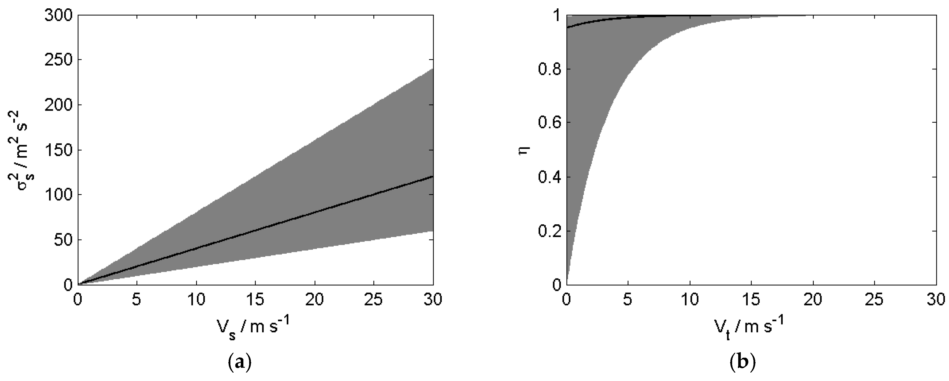
Qualitative illustrations of the observed trends summarised in Table 4. The black lines represent the median value whereas the shaded grey areas depict the spread. In (c,d), the areas of darker shade with the solid median line represent the mid-troposphere between the 700 mb and 200 mb pressure levels where the results in Table 4 were shown to be valid. (a) σ2s vs. Vs; (b) η vs. Vt; (c) σ2t vs. pressure level; (d) ε vs. pressure level.
Figure 14.
Qualitative illustrations of the observed trends summarised in Table 4. The black lines represent the median value whereas the shaded grey areas depict the spread. In (c,d), the areas of darker shade with the solid median line represent the mid-troposphere between the 700 mb and 200 mb pressure levels where the results in Table 4 were shown to be valid. (a) σ2s vs. Vs; (b) η vs. Vt; (c) σ2t vs. pressure level; (d) ε vs. pressure level.


Table 1.
Significance checks conducted on the computed statistics.
| Condition | Test, Confidence Level | Null Hypothesis | Action Taken If Null Hypothesis Is Not Rejected |
|---|---|---|---|
| Vt = 0 | t test (two-tailed), 95% | ; | Discard ϕ and η. |
| σ2t → 0 | χ2 test (upper tail), 95% | σ2t < 0.01Vt2 | Discard ε, θ, and η. |
| ε = 0 | F test (two-tailed), 95% | λmin = λmaj | Discard θ and η. |
Table 2.
Observed values of k considering all eleven pressure levels.
| n = 55; p = 0.02 kcrit = 5 | |
|---|---|
| Coefficient | k |
| L | 8 |
| M | 7 |
| N | 3 |
| C | 9 |
| A | 2 |
| B | 6 |
Table 3.
Observed values of k considering only the middle troposphere between the 700 mb and 200 mb pressure levels.
Table 3.
Observed values of k considering only the middle troposphere between the 700 mb and 200 mb pressure levels.
| n = 30; p = 0.02. kcrit = 4 | |
|---|---|
| Coefficient | k |
| L | 0 |
| M | 0 |
| N | 1 |
| C | 2 |
| A | 0 |
| B | 3 |
Table 4.
Summary of the characteristics of σ2s, σ2t, ε, and η with respect to Vs, Vt and pressure level.
Table 4.
Summary of the characteristics of σ2s, σ2t, ε, and η with respect to Vs, Vt and pressure level.
| Variance Statistic | Dependency on: | ||
|---|---|---|---|
| Vs | Vt | Pressure Level | |
| σ2s | Yes | No | |
| σ2t | No | Yes | |
| ε | No | Yes | |
| η | Yes | No | |
© 2018 by the authors. Licensee MDPI, Basel, Switzerland. This article is an open access article distributed under the terms and conditions of the Creative Commons Attribution (CC BY) license (http://creativecommons.org/licenses/by/4.0/).
Share and Cite
MDPI and ACS Style
Tieo, J.-J.; Koh, T.-Y.; Skote, M.; Srikanth, N. Variance Characteristics of Tropical Radiosonde Winds Using a Vector-Tensor Method. Energies 2018, 11, 137. https://doi.org/10.3390/en11010137
AMA Style
Tieo J-J, Koh T-Y, Skote M, Srikanth N. Variance Characteristics of Tropical Radiosonde Winds Using a Vector-Tensor Method. Energies. 2018; 11(1):137. https://doi.org/10.3390/en11010137
Chicago/Turabian StyleTieo, Jing-Jin, Tieh-Yong Koh, Martin Skote, and Narasimalu Srikanth. 2018. "Variance Characteristics of Tropical Radiosonde Winds Using a Vector-Tensor Method" Energies 11, no. 1: 137. https://doi.org/10.3390/en11010137
Note that from the first issue of 2016, this journal uses article numbers instead of page numbers. See further details here.