State-Space Approximation of Convolution Term in Time Domain Analysis of a Raft-Type Wave Energy Converter


Department of Fluid Control and Automation, Harbin Institute of Technology, Harbin 150001, China
*
Author to whom correspondence should be addressed.
Energies 2018, 11(1), 169; https://doi.org/10.3390/en11010169
Submission received: 22 November 2017
/
Revised: 26 December 2017
/
Accepted: 3 January 2018
/
Published: 10 January 2018
(This article belongs to the Special Issue Wave Energy Potential, Behavior and Extraction)
Abstract
:Two methods, frequency domain analysis and time domain analysis, are widely applied to modeling wave energy converters (WECs). Frequency domain analysis can evaluate the performance of WECs quickly and efficiently, while it refers to a linear model. When it comes to investigations on nonlinear characteristics of the power take-off (PTO) unit of WECs or control for improving the WECs’ performance, time domain analysis based on a state-space approximation for the convolution term is more desirable. In this paper, a state-space approximation of the convolution term in a time domain analysis of a raft-type WEC consisting of two rafts and a PTO unit is presented. The state-space model is identified through regression in the frequency domain. Verification of such a type of time domain analysis is conducted by comparison of its simulation results with those calculated by using a frequency domain analysis, and there is a good agreement. Finally, the effects of PTO parameters, wave frequency, surge and heave motions of the joint, and quadratic damping PTO on the power capture ability of the raft-type WEC are investigated.
1. Introduction
Wave energy with its renewable and non-polluting properties is wildly explored in many countries [1,2]. In order to extract and utilize wave energy, many scholars have proposed varieties of energy conversion devices. The most notable device is the point-absorbing wave energy converter (WEC), which has been studied since the late 1970s [3]. Based on the mechanism of the point-absorbing WEC, other types of WECs appeared, such as oscillating-water column WEC, pendulum WEC, and raft-type WEC [4].
The raft-type WEC is a semi-submerged offshore structure, composed of a series of rafts, which are articulated end to end by the joints containing hydraulic power take-off (PTO) units [5]. The device is deployed in a direction parallel to the propagation direction of the incident waves. Under the action of the incident waves, each raft outputs surge, heave, and pitch motions, while only the relative pitch motion between the rafts around the joint forces the hydraulic cylinders to pump high-pressure (HP) oil. Then, the HP oil drives the hydraulic motor shaft to rotate, and this rotation forces the generator to produce electricity [1].
Research on the raft-type WEC originated in 1979, when Haren and Mei [6,7,8] adopted a two dimensional fluid-structure coupling model to study the contouring rafts by modeling the PTO unit as a linear PTO system. Their contribution included the power absorption efficiency of one raft hinged at a wall in long wave conditions, multiple rafts with variable lengths in shallow water wave conditions, and a three-raft system in both shallow and deep-water wave conditions. By assuming that the raft was a “limp-beam” model, Farley [9] explored the energy conversion ability of a flexible resonant raft.
In later years, the McCabe Wave Pump, another type of raft-type device, composed of three rectangular barges hinged together, where the relative pitch motion between the fore, aft, and the middle barges is used to generate electricity or produce potable water, was studied by Kraemer [10] and Nolan et al. [11]. Kraemer’s finding showed that the pitch motion of the hinged barges could be maximized by altering the ratio of the length of barges and the wavelength. Nolan et al. adopted the bond graph method to model a more complicated PTO unit including a non-linear damper for the McCabe Wave Pump. In order to solve the dynamics of multi-body WECs, Paparella et al. [12] applied pseudo-spectral methods to the McCabe Wave Pump using both differential and algebraic equations (DAEs) formulation and ordinary differential equations (ODEs) formulation. Their results showed that pseudo-spectral methods are computationally more stable and require less computational effort for short time steps.
The Pelamis WEC manufactured by Pelamis Wave Power Company is another successful application of the raft-type device. The company has conducted many valuable researches on the Pelamis device including testing on a laboratory scale and under real sea conditions [13,14,15]. The Pelamis device can use both the relative pitch and relative yaw motions around its joints to generate electricity. The current model, the Pelamis P2 composed of five cylindrical modules, with a total length of 180 m, has a maximum capture width as large as 150% of its ‘displacement width’ [15].
With the concept of Pelamis or Pelamis-like, Thiam and Pierce [16,17,18] investigated the radiation loss in a Pelamis-like WEC by assuming an infinitely long flexible circular cylinder floating on the surface of an infinitely deep ocean. Their researches showed that the influence of radiation losses is significant if the overall length of the device is much larger than the wavelength of the incident wave.
In recent years, Zheng et al. [19,20] have presented a six-degree-of-freedom (six-DOF) frequency domain model for a raft-type wave energy conversion device of an elliptical cross section. In their research, the effects of the raft radius of gyration and axis ratio of the raft on the wave energy conversion ability were explored, and they conducted a theoretical study on the maximum power that the raft-type device could extract by using a linear PTO model. To investigate the effect of latching control, a six-DOF time domain model based on Cummins’ equation for the raft-type device was also presented by Zheng et al. [20].
By using the Lagrange multiplier technique, Sun et al. [21] provided a frequency domain linear diffraction model to investigate the responses of interconnected floating bodies. Then, Sun et al. [22,23] applied this frequency domain linear diffraction model to a raft-type-like WEC M4 in regular waves and irregular multi-directional waves to predict relative pitch rotation and power capture. Their results showed a good agreement of relative rotation and power capture with experiments. More recently, Stansby et al. [24] presented a time domain linear diffraction model based on Cummins’ method for the raft-type-like WEC M4 to investigate large capacity multi-float configurations.
So far, most of the previous researches on the raft-type WEC have been conducted by using a frequency domain analysis with the assumption of a linear model, or using a time domain analysis based on Cummins’ equation with a convolution term. When the research includes control to improve the WEC’s performance, a time domain analysis with the convolution term approximated by a state-space model is more desirable, since such a type of time domain analysis is well suited for controller design and simulation [25,26]. Recent literature [27] has presented such a type of time domain analysis for a raft-type WEC consisting of two rafts and a PTO unit. However, the details of how to reformulate the convolution term into a state-space model and the realization of such a state-space model were not reported. This paper focuses on providing the details regarding the state-space modeling procedure for approximating the convolution term in the time domain analysis of the raft-type WEC. Besides, based on such a type of time domain analysis, the effects of PTO parameters, wave frequency, surge and heave motions of the joint, and quadratic damping PTO on the power capture ability of the raft-type WEC are explored.
2. Description of the Device
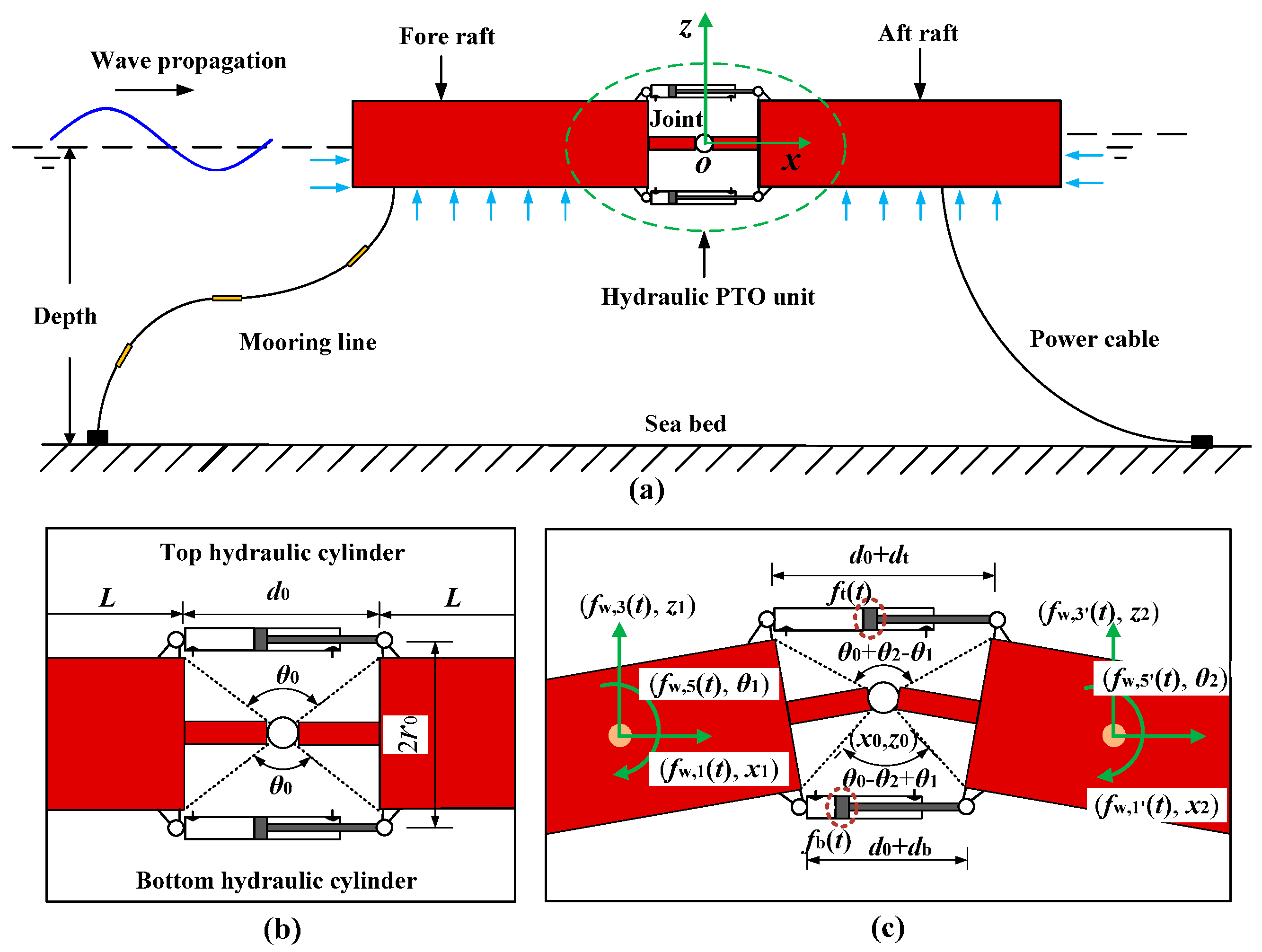
Figure 1 presents a raft-type WEC composed of two floating rafts and a hydraulic PTO unit. The two rafts with a cylindrical shape are articulated by a joint with a gap d0 between them, as shown in Figure 1b. The length, diameter, and density are denoted as L, D, and ρ0, respectively. The motion characteristic of the device is formulated in a Cartesian coordinate (x, y and z) system with its origin O coincident with the center of the joint, where the z-axis is in the vertical direction, while the x- and y-axes are taken along the length and the diameter direction of the rafts in still water, respectively, as shown in Figure 1a. For the fore raft, the displacements are labeled as x1-surge, z1-heave, and θ1-pitch. For the aft raft, the displacements are labeled as x2-surge, z2-heave, and θ2-pitch. The surge and heave displacements of the joint are denoted as x0 and z0, as shown in Figure 1c.
The forces acting on each raft are shown in Figure 1c. The wave force on mode j of the rafts is denoted as fw,j (t) (here, subscript j = 1, 3, and 5 indicate the surge, heave, and pitch modes of the fore raft, respectively; j = 1′, 3′, and 5′ indicate the surge, heave, and pitch modes of the aft raft, respectively). As the wave passes along the length of the rafts, the rafts output a relative pitch motion around the joint, which drives the hydraulic PTO unit to convert wave energy.
3. Frequency Domain Analysis
By assuming the hydraulic cylinder as a linear damper plus a linear stiffness, Liu et al. [27] adopted a generalized displacement vector x(t) = [x0 z0 θ1 θ2]T to describe the motion characteristic of the device and given a four-DOF frequency domain model for waves in the positive x-direction based on the Lagrange’s equations, which can be written as:
where ω is the wave frequency; “i” is the imaginary unit; M is the generalized mass matrix; Aadd(ω) is the generalized added mass matrix; B(ω) is the generalized radiation damping matrix; K is the generalized hydrostatic restoring stiffness matrix; Cpto and Kpto are the damping matrix and stiffness matrix of the PTO unit, respectively; X(ω) is the complex amplitude of the generalized displacement vector x(t); and Fe(ω) is the complex amplitude of the generalized wave excitation force vector. Their expressions are given in Appendix A.
3.1. Frequency Response Function
The frequency response function (FRF) of the wave amplitude-to-complex amplitude of the generalized displacement vector, G(ω), can be described by [27]:
where aw is the wave amplitude and Γe(ω) is the complex generalized excitation force coefficient vector (force vector per unit incident wave amplitude). The expression of Γe(ω) is given in Appendix A.
The FRF of the wave amplitude-to-complex amplitude of relative pitch velocity, Gv_rp, is:
where ζ = [0 0 1 −1].
3.2. Power Capture Ability
The average power captured by the PTO unit from the incident wave is:
The time-average flux of energy transported by a regular wave per unit wave crest length in a finite water depth is [28]:
where ρ is the density of sea water; g is the gravity acceleration; h is the water depth; and k is the wave number.
The capture width ratio is a significant parameter to evaluate the power capture ability of a WEC. In the study of the raft-type-like WEC M4, Sun et al. [22,23] normalized the capture width by wavelength to obtain the capture width ratio. Here, we also adopt the same definition, since this definition of the capture width ratio enables a comparison with theoretical maxima, e.g., 3/2π in heave and pitch and/or surge for a point absorber [28] and 4/3π for a slender two-raft WEC [29]. Thus, the capture width ratio is:
where λ is the wavelength at frequency ω.
4. Time Domain Analysis
When the model refers to a linear model, the frequency domain analysis shown in the above section is convenient and efficient to evaluate the performance of the device in a prescribed sea state. However, sometimes, due to the relatively low capture width ratio of a WEC without control, it is imperative to do more thorough researches on its performance, for instance, incorporating the nonlinear characteristics of the hydraulic PTO unit or the control; at this time, the frequency domain analysis is limited, and therefore, a time domain analysis is more desirable. Taking the inverse Fourier transform of Equation (1), the time-domain model of the device is shown as below:
where Aadd(∞) is the limiting value of the generalized added mass matrix Aadd(ω) for ω = ∞; fe(t) is the generalized wave excitation force vector; fpto(t) is the generalized force vector applied by the PTO unit; and h(t) is the retardation function matrix. The time and frequency domain representations of the retardation function matrix are [28]:
In irregular waves, the wave excitation force acting on the mode j of the rafts can be expressed as [28]:
where ωn, εn, and aw(ωn) are the wave frequency, random phase angle, and wave amplitude of the n-th wave component, respectively.
The time domain generalized excitation force vector can be obtained by [27]:
where l is the distance between the mass center of the raft and the joint.
The force vector applied by the PTO unit can be written as:
4.1. State-Space Model of Convolution Term
The time domain motion equation presented above contains a convolution term, which denotes the fluid memory effect. Performing the simulation of such a type of time domain model can be time-consuming and may require significant amounts of computer memory, as demonstrated in Taghipour et al. [25,30]. What is worse is that it is not suited for controller analysis and design. For these reasons, different methods of approximating the convolution term have been proposed in many literatures [25,30,31]. One approach is to use a linear-time-invariant parametric model in a state-space form to substitute the convolution term by frequency domain identification [25,30,31]. The convolution term in Equation (7) for calculating the fluid-memory effect can be described by μ(t):
For the convolution term μ(t), it also has a form as:
For each element μp,q(t) in the convolution term μ(t) can be replaced by a state-space model [29,32].
where p and q vary from 1 to 4, and x(q)(t) is the q-th element of the generalized displacement vector x(t); the sizes of matrices As(p,q), Bs(p,q), and Cs(p,q) are (np,q × np,q), (np,q × 1), and (1 × np,q), respectively; and np,q is the number of states corresponding to the state vector xs(p,q).
By using Equation (16) to replace all the elements in the convolution term μ(t), sixteen state-space models are presented. Then, for reducing the model complexity and computational load, four state-space models can be assembled by these sixteen state-space models to replace each convolution term μp(t), and finally, a total state-space model can be assembled by the four state-space models. Figure 2 shows the general idea of assembling the state-space model. Thus, the convolution term μp(t) can be rewritten as:
where matrices As(p), Bs(p), and Cs(p) are assembled by matrices As(p,q), Bs(p,q), and Cs(p,q), respectively; the state vector xs(p) is assembled by state vectors xs(p,q); the sizes of matrices As(p), Bs(p), Cs(p), and xs(p) are (), (), (), and (), respectively. The expressions of As(p), Bs(p), Cs(p), and xs(p) are shown in Appendix A.
Therefore, the total state-space model of Equation (14) can be written as:
where matrices As, Bs, and Cs are assembled by matrices As(p), Bs(p), and Cs(p), respectively; the state vector xs is assembled by state vectors xs(p); and the sizes of matrices As, Bs, Cs, and xs are (), (), (), and (), respectively. The expressions of As, Bs, Cs, and xs are shown in Appendix A.
The next task is to obtain matrices As(p,q), Bs(p,q), and Cs(p,q). It can be seen from Equation (16) that the Laplace transform of the retardation function hp,q(t) is the transfer function of the system with scalar input and scalar output μp,q(t). Thus, the relationship between the state-space model and the transfer function is:
The transfer function can also be described by:
where s = −iω.
Therefore, the transfer function matrix of the total system with vector input and vector output μ(t) (see Equation (18)) can be expressed by:
Equations (9), (19), and (20) show a general idea of how to obtain the constant matrices As(p,q), Bs(p,q), and Cs(p,q) by identification using the generalized added mass matrix Aadd(ω) and radiation damping matrix B(ω). Moreover, for the two rafts with the same geometric parameter, it should be mentioned that some elements of the symmetrical transfer function matrix H(s) would satisfy the following relationships: H12(s) = H21(s) = 0, H13(s) = H14(s), H23(s) = −H24(s), and H33(s) = H44(s). Therefore, the identification only need to be carried out for H11(s), H13(s), H22(s), H23(s), H33(s), and H34(s), i.e., to determine the transfer function matrix H(s) of the total system, the identification procedure only needs to be carried out six times.
4.2. Transfer Function Estimation Using Regression in Frequency Domain
For a single input single output transfer function , a rational parametric model can be estimated by using the frequency domain regression from non-parametric data of the FRF . Assuming the estimated has a form of:
where ϕ is a vector containing the estimated parameters, and defined as:
It can be seen from Equation (22) that the problem of frequency domain identification is to find the order ν and the relative degree ν − γ of , and to determine the parameter vector ϕ that gives the best non-linear least square (NL-LS) fitting to the frequency response.
where wn is the weighting coefficient and “arg min” represents the minimizing argument.
Once the order ν and the relative degree ν − γ are chosen, the NL-LS fitting problem can be solved by an iterative method proposed by Sanathanan and Koerner [33]. The iterative method runs by using the polynomial corresponding to the previous iteration as the weight, and thus, the NL-LS fitting problem defined in Equation (24) is simplified as:
where
The linear problem described in Equation (25) can be solved by Matlab function invfresqs with the option of using a vector of weighting coefficients. Usually, the iterative procedure is implemented starting with αn,g = 1, and after a few iterations Qpq (−iω, ϕg) ≈ Qpq (−iω, ϕg−1). Then, the optimal parameter of vector ϕ can be determined as ϕ* = ϕg. Thus, the parametric model can be obtained. Then, the constant matrices As(p,q), Bs(p,q), and Cs(p,q) of the state-space model can be determined by using the Matlab function tf2ss. Thereafter, the matrices As, Bs, and Cs can be assembled by the formulations shown in Appendix A. Finally, the identified state-space model can be applied to replace the convolution term in the time domain model.
4.3. Power Capture Ability
The instantaneous power captured by the PTO unit is:
The average power captured in the time domain is:
where t0 is a moment when the device has come into a steady state of motion and T is the wave period.
The capture width ratio in the time domain is:
5. Numerical Results and Discussion
In this section, the identification of the state-space model is firstly carried out. Then, verification of the time domain analysis is performed by comparing its simulation results with those calculated by using the frequency domain analysis. Thereafter, the effects of PTO parameters, wave frequency, surge and heave motions of the joint, and quadratic damping PTO on the performance of the device are investigated and discussed.
5.1. Identification of State-Space Model
Before performing the time domain analysis, identification of the state-space model needs to be carried out. The identification is carried out in the frequency domain by using an iterative method. The general assumptions made in the hydrodynamic analysis of the device are: (1) the rafts are considered as rigid bodies; (2) the fluid is incompressible inviscid; and (3) the flow is irrotational. A truncated frequency ranging from 0.01 rad/s to 9 rad/s is adopted to calculate the hydrodynamic parameters (i.e., the added mass auj(ɷ), the radiation damping buj(ɷ), and the complex excitation force coefficient Γj(ɷ)) in ANSYS AQWA [34], commercial hydrodynamic software based on three dimensional radiation/diffraction theory.
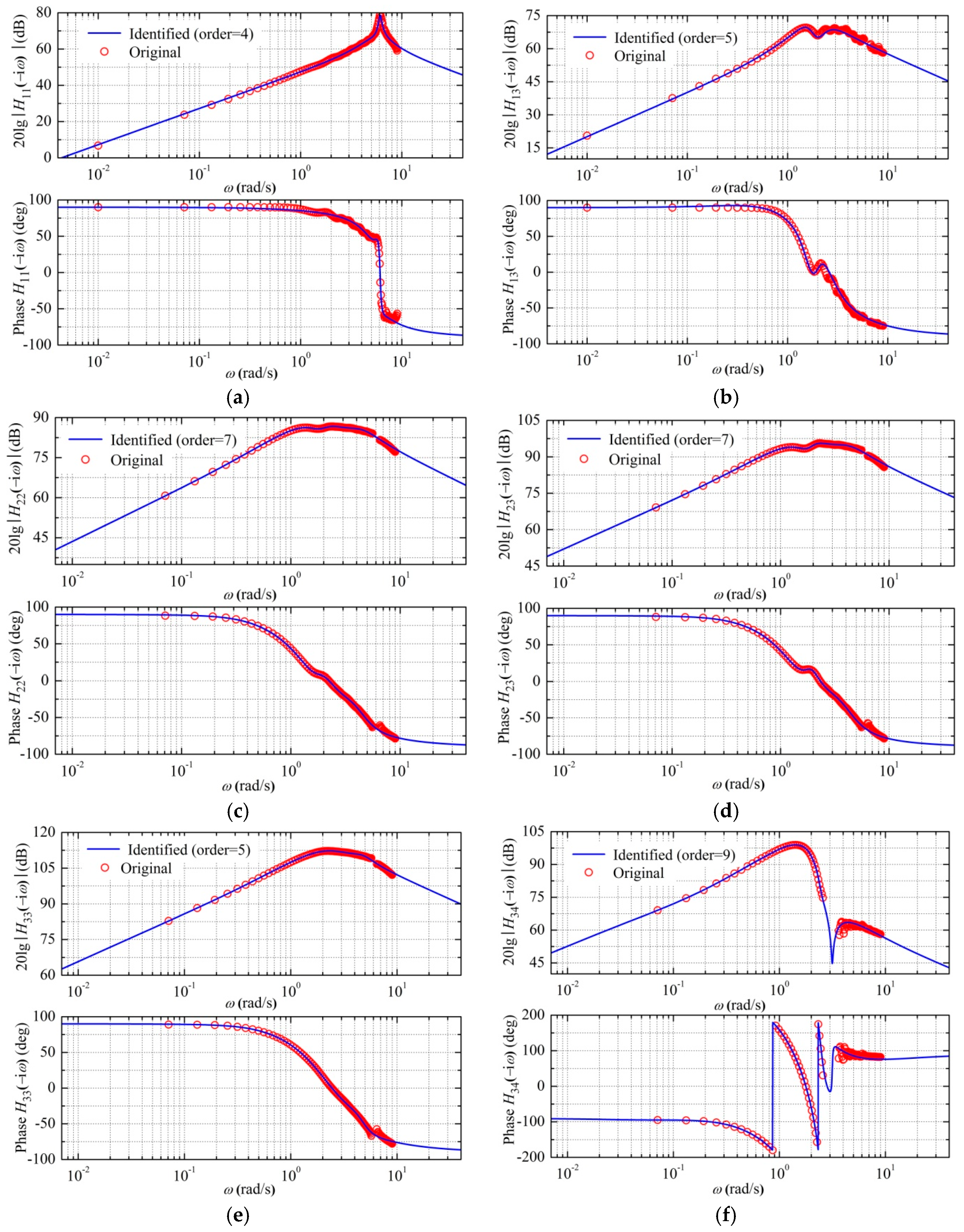
Figure 3 shows the identification results of the retardation functions H11(−iω), H13(−iω), H22(−iω), H23(−iω), H33(−iω), and H34(−iω) for the device with structure parameters L = 10 m, D = 1 m, d0 = 1 m, and ρ0 = 512.5 kg/m3. The sizes of constant matrices As, Bs, and Cs are 87 × 87, 87 × 4, and 4 × 87, respectively, which are not shown here for their large sizes. The original data of retardation functions H11(−iω), H13(−iω), H22(−iω), H23(−iω), H33(−iω), and H34(−iω) calculated by Equation (9) are also presented in Figure 3. It can be seen that there is a good agreement between the identification results and those obtained by Equation (9).
5.2. Validation of Time Domain Analysis
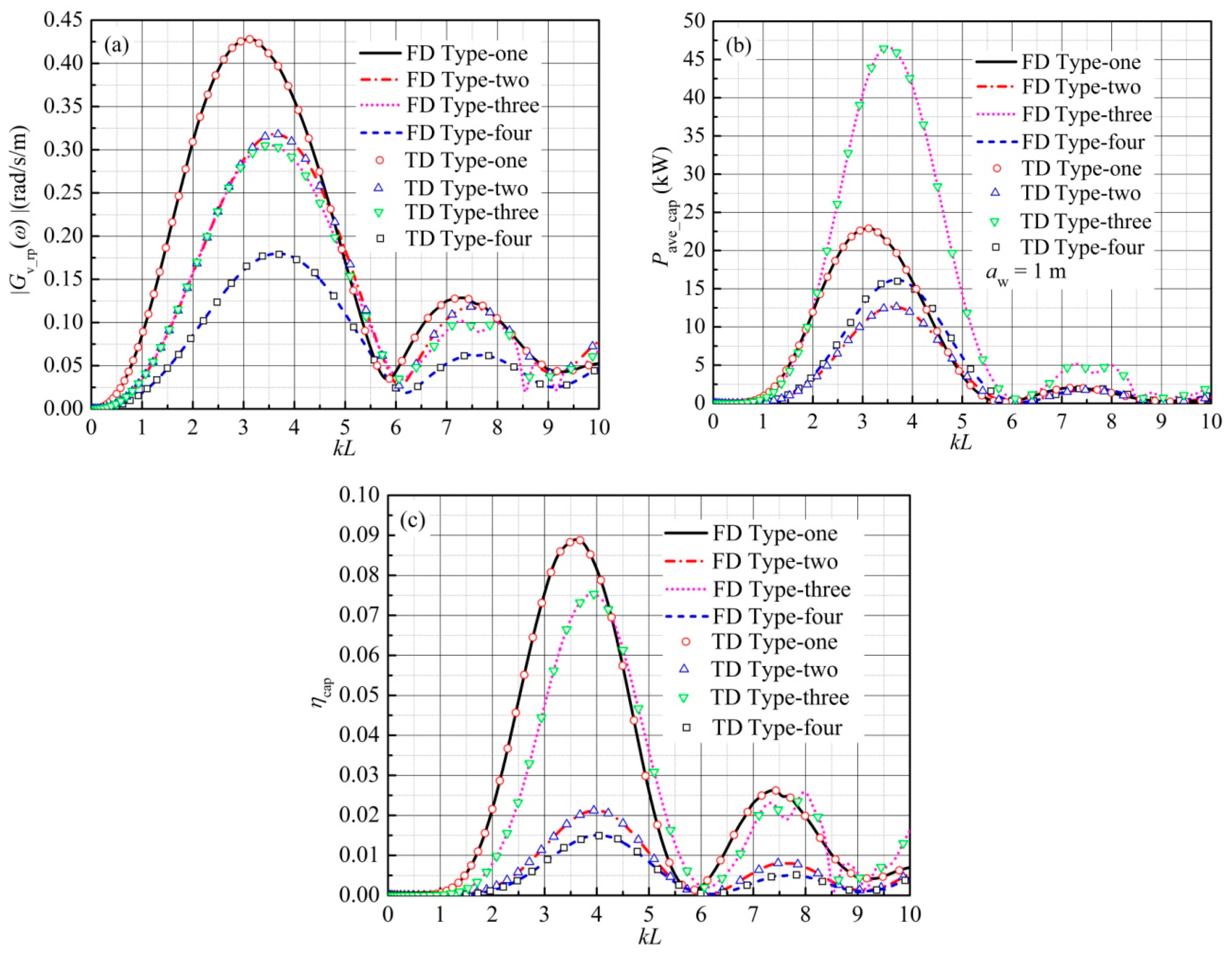
The time domain model (see Equation (7)) can be solved by the fourth-order Runge-Kutta method. Thus, the FRF of the wave amplitude-to-complex amplitude of relative pitch velocity and the capture width ratio can be obtained. In the frequency domain analysis, they can be calculated quickly by Equations (3) and (6), respectively. The stiffness of the PTO unit is assumed to be zero in this work, unless otherwise specified. Four types of structure parameters are considered, as shown in Table 1.
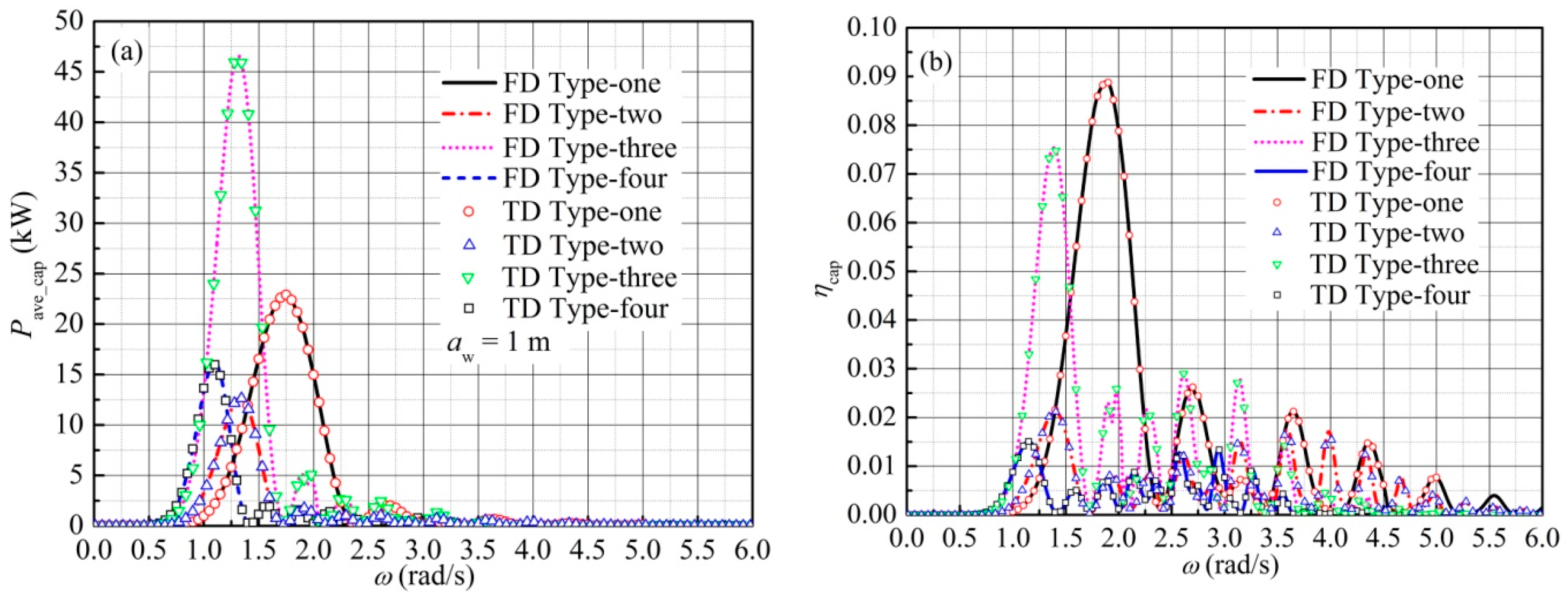
Figure 4 shows the comparison of the performance of the devices with these four types of structure parameters between the frequency domain calculations and the time domain simulations. It can be seen from Figure 4 that there is a good agreement between the results obtained by using the time domain analysis and those calculated by using the frequency domain analysis.
5.3. Numerical Results in Regular Waves
5.3.1. Influence of Wave Frequency
One can also see from Figure 4b that, for the devices with these four types of structure parameters, the optimal ratio kL corresponding to the peak captured power ranges from 3.1163 to 3.6715, which is shown explicitly in Table 1. The optimal ratio of raft length to wavelength varies from 0.4960 to 0.5843, whereas the corresponding resonant frequency of relative pitch velocity varies from 1.7485 rad/s to 1.0957 rad/s. Figure 5 shows the variation of average captured power and capture width ratio with wave frequency.
It can be seen from Figure 5 that the captured power and the capture width ratio are relatively large when the wave frequency gets close to the corresponding resonant frequency of the device, whereas they are rather small at the wave frequency far away from the resonant frequency. Therefore, in order to maximize the captured power and the capture width ratio, the resonant frequency of the designed device should be close to the considered wave frequency. The resonant frequency depends on the raft mass, the rotary inertia about the mass centre, the added mass, the radiation damping, the hydrostatic restoring stiffness, and the damping coefficient and stiffness of the PTO unit, among which the added mass, the hydrostatic restoring stiffness, the raft mass, and rotary inertia mainly depend on the raft size when the material of the raft is chosen. If there is no control included in the PTO unit, the arrival of resonance is usually at the cost of a relatively large raft size, which is shown explicitly in Table 1. The resonant frequency of the device with a type-one parameter is 1.7485 rad/s, whereas the resonant frequency of that with a type-four parameter is 1.0957 rad/s; however, the raft volume of the device with a type-four parameter is twelve times as large as that with a type-one parameter.
5.3.2. Influence of Mounting Position r0
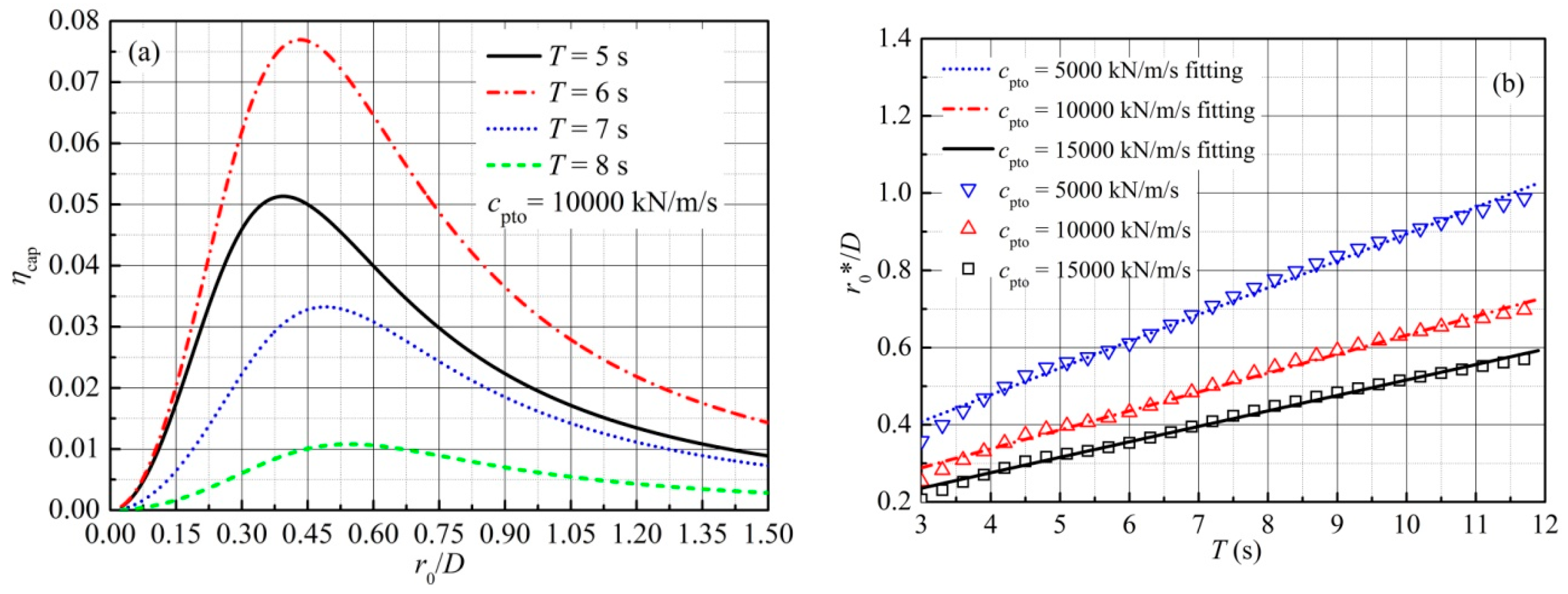
As shown in Equations (4) and (6), the mounting position r0 of hydraulic cylinder is a key parameter influencing the capture width ratio of the device. It is assumed that the mounting position r0 is not confined to the diameter of the rafts. The power capture ability of the device is examined by using the time domain analysis over a wide range of mounting positions r0. Figure 6a shows the variation of the capture width ratio of the device with a type-four parameter with the mounting position normalized by the diameter of the raft at four different wave periods. It can be seen that the capture width ratio ηcap increases with an increasing normalized mounting position r0/D, and then decreases after reaching a peak value. This is not surprising. As shown in Equation (A.6), there is a quadratic function relationship between the rotational damper 2r02cpto and the mounting poison r0. For any specified wave period T and any specified damping coefficient cpto, a too large mounting position r0 (i.e., too large rotational damping 2r02cpto) would lead to a small relative pitch motion, and consequently, the device outputs a little power; whereas a too small mounting position r0 (i.e., too small rotational damping 2r02cpto) would induce a small PTO force, which also results in a little captured power. Therefore, for any specified wave period and any specified damping coefficient cpto, there exists an optimal normalized mounting position r0*/D, which corresponds to a peak capture width ratio ηcap*.
The variation of the optimal normalized mounting position r0*/D with wave period T is illustrated in Figure 6b. It is found that the optimal normalized mounting position r0*/D presents an approximately linear relationship with wave period, and a smaller damping coefficient cpto gives a larger gradient of the approximate linear relationship.
5.3.3. Influence of Damping Coefficient cpto and Stiffness kpto
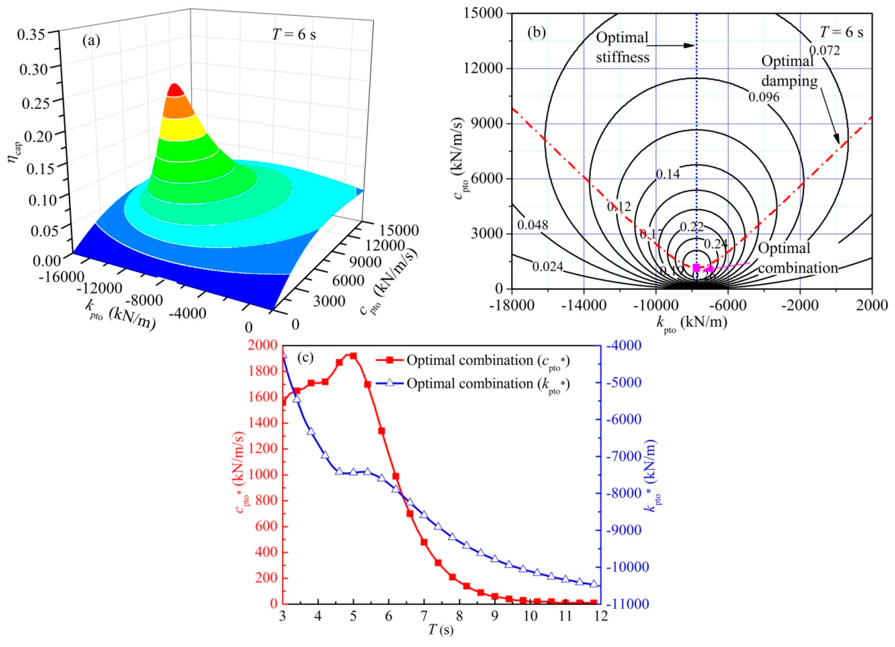
In the above sections, the stiffness kpto is assumed to be zero, while in fact, the stiffness plays a significant role in power extraction. In order to see how the stiffness kpto and the damping coefficient cpto affect the power capture ability of the device, the capture width ratio is examined by using the time domain analysis over a wide range of damping coefficients cpto and stiffnesses kpto. Figure 7 shows the influence of the damping coefficient cpto and stiffness kpto on the capture width ratio of the device with a type-four parameter.
It can be seen from Figure 7a,b that, for a specified wave period T, there exists an optimal stiffness kpto*, which only depends on the wave period T. For a specified wave period T and a specified stiffness kpto, there exists an optimal damping coefficient cpto*. The optimal damping coefficient cpto* decreases with increasing stiffness kpto, and then increases after reaching a minimum value, and is symmetric to the optimal stiffness kpto*, as shown in Figure 7b. When the optimal damping coefficient cpto* is obtained in the condition of optimal stiffness kpto*, an optimal combination of the optimal damping coefficient and the optimal stiffness is achieved. This optimal combination could improve the power extraction ability significantly. As is shown in Figure 7a,b, the capture width ratio obtains a value of 0.0769 at kpto = 0 kN/m and the corresponding optimal damping coefficient, whereas it can reach 0.2868 at the optimal combination, i.e., an increase of more than 270%. Therefore, if the stiffness kpto of the PTO unit can be adjusted to be an optimal stiffness kpto* in the varying wave states, which makes the resonant frequency close to the considered wave frequency, the capture width ratio of the device can be improved dramatically. However, as it is revealed in [35], the nonlinear viscous damping would play an important role in the dynamic response of a WEC, especially in the vicinity of the resonant frequency. Hence, the present numerical model based on inviscid flow theory may overestimate the captured power, and the capture width ratio may thus be overpredicted.
The variation of the optimal damping coefficient cpto* and the optimal stiffness kpto* in the optimal combination with wave period is presented in Figure 7c. It can be learned from Figure 7c that the optimal stiffness kpto* in the optimal combination is normally negative, which means that the PTO unit may output power to the rafts in some period of its cycle. To be scientific, it is a kind of reactive control [28], but it is difficult to implement practically without a complicated PTO unit. It can also be seen from Figure 7c that the optimal damping coefficient cpto* in the optimal combination increases with the increase of wave period, then decreases after reaching a peak value, whereas, generally, the optimal stiffness kpto* in the optimal combination decreases monotonously.
5.3.4. Influence of Surge and Heave Motions of Joint
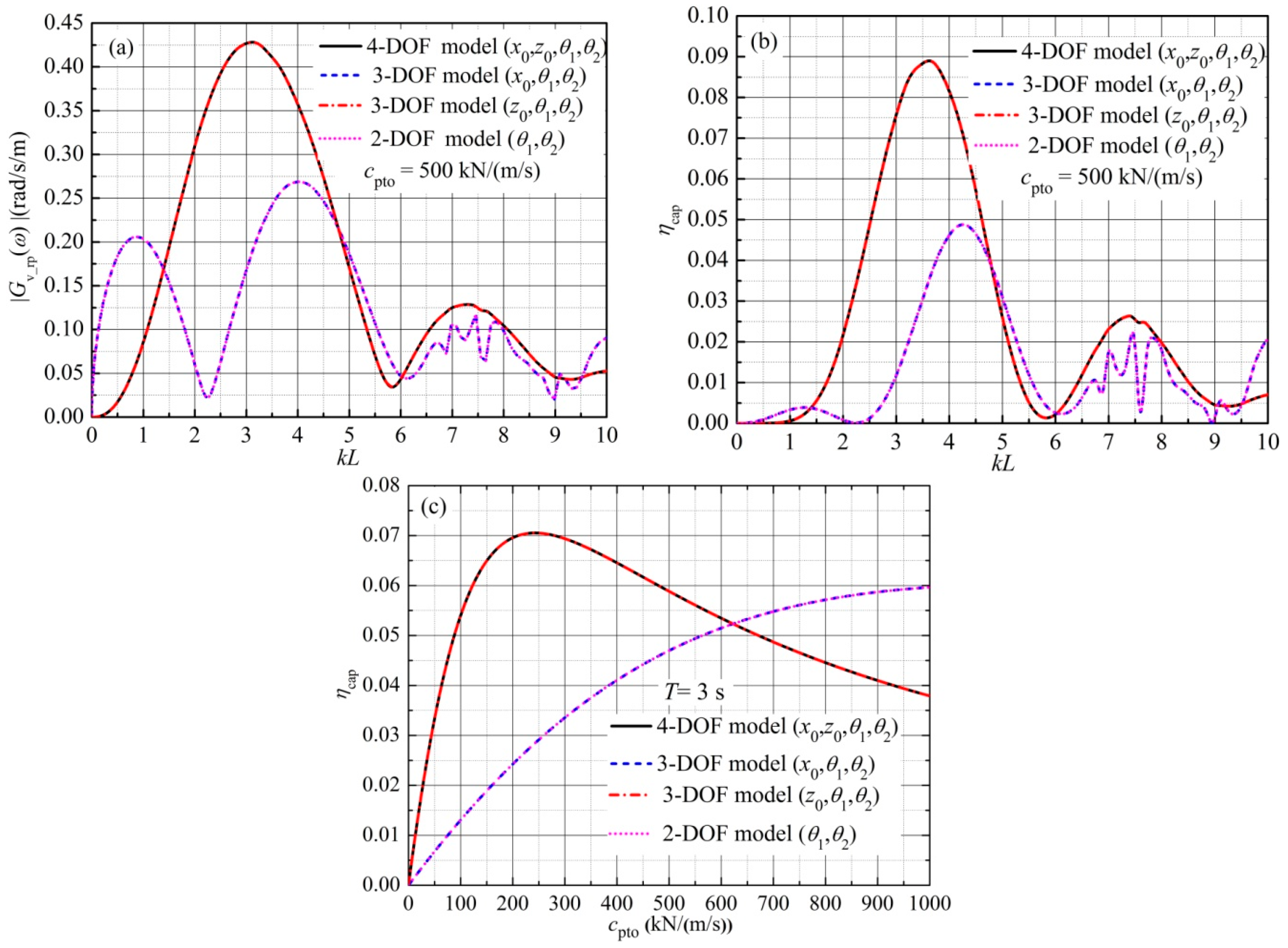
To investigate the effect of surge and heave motions of the joint on the performance of the device, we remove the surge and heave motions of the joint, and take the motion system as a two-DOF model and a three-DOF model, and then compare their results with those of the full four-DOF model. Figure 8a presents the FRF of the wave amplitude-to-complex amplitude of the relative pitch velocity Gv_rp for the device with a type-one parameter. Figure 8b shows the corresponding capture width ratio ηcap, obtained by the model with and without a consideration of surge and heave motions of the joint, whereas the variation of capture width ratio ηcap with the damping coefficient cpto is presented in Figure 8c.
It can be seen from Figure 8 that the results obtained by the full-four DOF model are almost overlaid by those obtained by the three-DOF model only removing the surge motion of the joint. However, the results obtained by the three-DOF model only removing the heave motion of the joint and those obtained by the two-DOF model removing both the surge and heave motions of the joint deviate greatly from those obtained by the full-four DOF model. This indicates that the surge motion of the joint has little effect on the performance of the device, whereas the heave motion of the joint makes a huge difference. This is, perhaps, not surprising based on physical intuition. For a deeper understanding, we can see from Table 1 that the resonant frequency of heave velocity is very close to that of relative pitch velocity, while the resonant frequency of surge velocity is far away from that of relative pitch velocity. In addition, the amplitude of FRF of the wave amplitude to heave velocity at the resonant frequency of heave velocity is largely higher than that of the wave amplitude to surge velocity at the resonant frequency of surge velocity. The information in Table 1 and Figure 8 reveals that the relative pitch mode shows stronger coupling with the heave mode than the surge mode. Therefore, the surge motion of the joint could be neglected. Thus, the motion equation of the device could be reduced to a three-DOF model only with the consideration of the heave motion of the joint and two pitch motions of the two rafts. Besides, by using the three-DOF model removing the surge motion of the joint to obtain the total state-space model for substituting the convolution term, the identification procedure only need to be carried out four times, which is more concise than the full four-DOF model.
5.3.5. Influence of Quadratic Damping PTO
In this section, the force applied by the PTO system is assumed to be quadratic damping. It can be written as:
where fx0(t), fz0(t), fθ1(t), and fθ2(t) are the PTO forces acting on the generalized modes x0, z0, θ1, and θ2, respectively; and β is the quadratic damping coefficient.
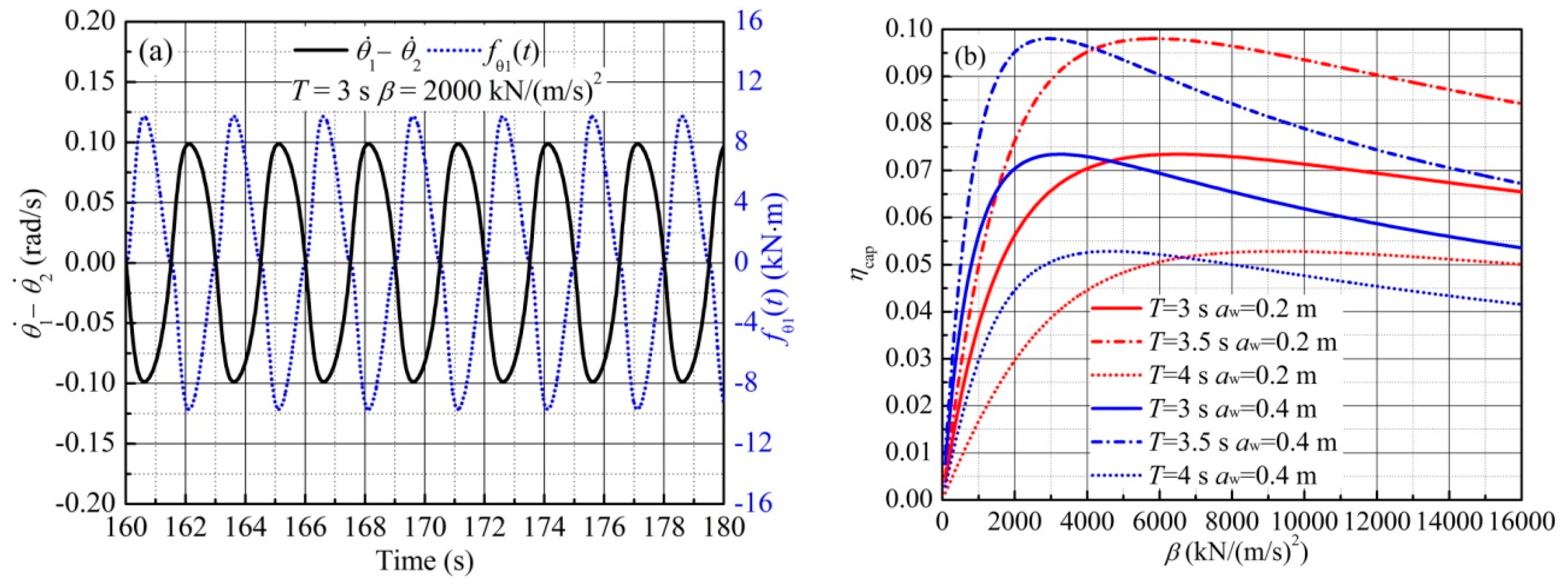
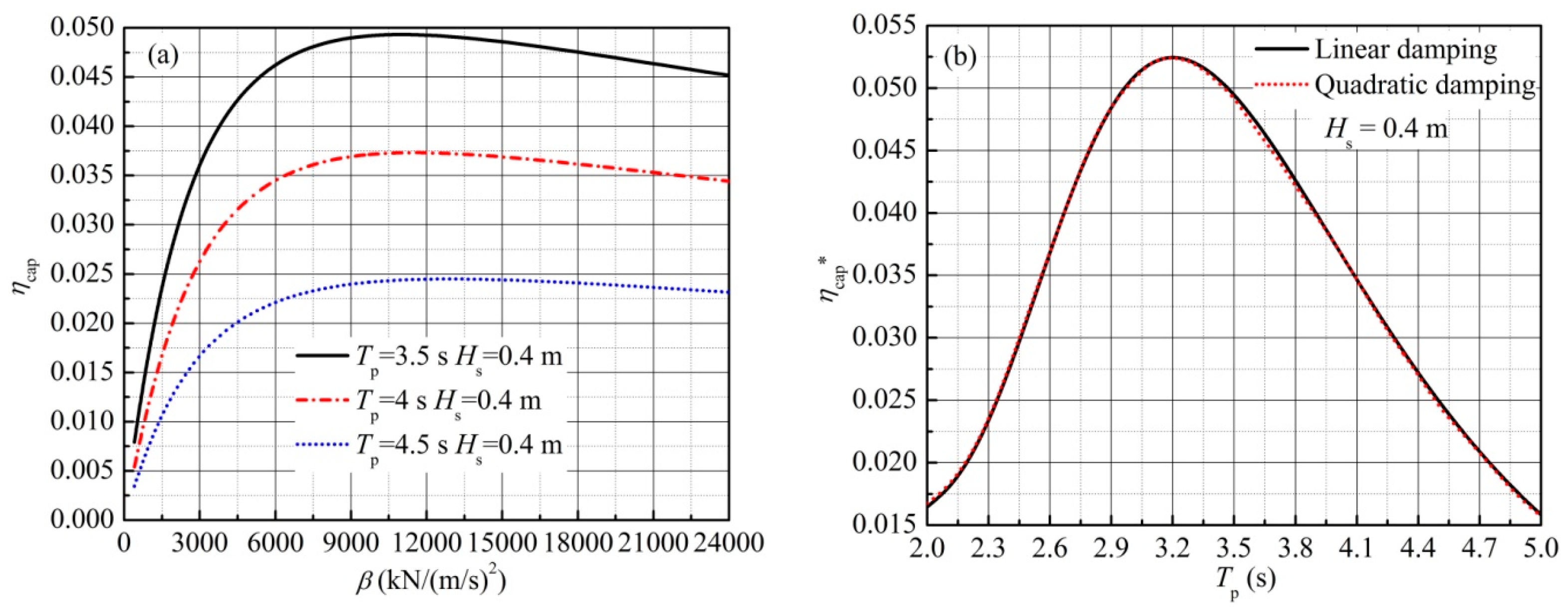
We apply the time domain analysis to explore the effect of quadratic damping on the performance of the device with a type-one parameter. Figure 9a shows how relative pitch velocity and PTO force vary with time, whereas the variation of capture width ratio with quadratic damping coefficient β is presented in Figure 9b.
It can be seen from Figure 9a that the relative pitch velocity presents nonlinear characteristics due to the nonlinear PTO unit. As shown in Figure 9b, the capture width ratio ηcap increases with an increasing quadratic damping coefficient β, and then decreases after reaching a peak value. For the wave states with the same period, a larger wave amplitude gives a higher capture width ratio at small quadratic damping coefficients β, while the peak capture width ratio ηcap* has the same value at different wave amplitudes.
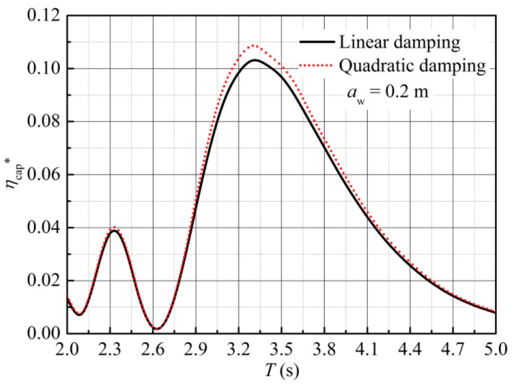
To recognize the difference in behaviour exhibited between linear damping and quadratic damping, we compare the peak capture width ratios obtained by using linear damping and quadratic damping. Figure 10 presents the comparison of peak capture width ratios ηcap* obtained by using linear damping and quadratic damping. It can be seen that the peak capture width ratio ηcap* obtained by using quadratic damping is slightly larger than that obtained by using linear damping, especially in the vicinity of wave period T = 3.3 s. For 2 s < T< 2.6 s or 2.6 s < T< 5 s, the difference in peak capture width ratios obtained by using linear damping and quadratic damping increases with increasing wave period, and then decreases after reaching a local maximum value. The maximum peak capture width ratio ηcap* obtained by using quadratic damping is 0.1086, whereas that obtained by using linear damping is 0.1031, and they are all obtained at wave period T = 3.3 s.
5.4. Numerical Results in Irregular Waves
We also investigate the performance of the device in irregular waves by using the time domain analysis. For the irregular wave computations, the Pierson–Moskowitz energy density spectrum as a function of the angular frequency is used to provide a good representation of the sea states. The Pierson–Moskowitz spectrum has the form [36]:
where Hs is the significant wave height and Tp is the peak wave period.
5.4.1. Influence of Mounting Position R0
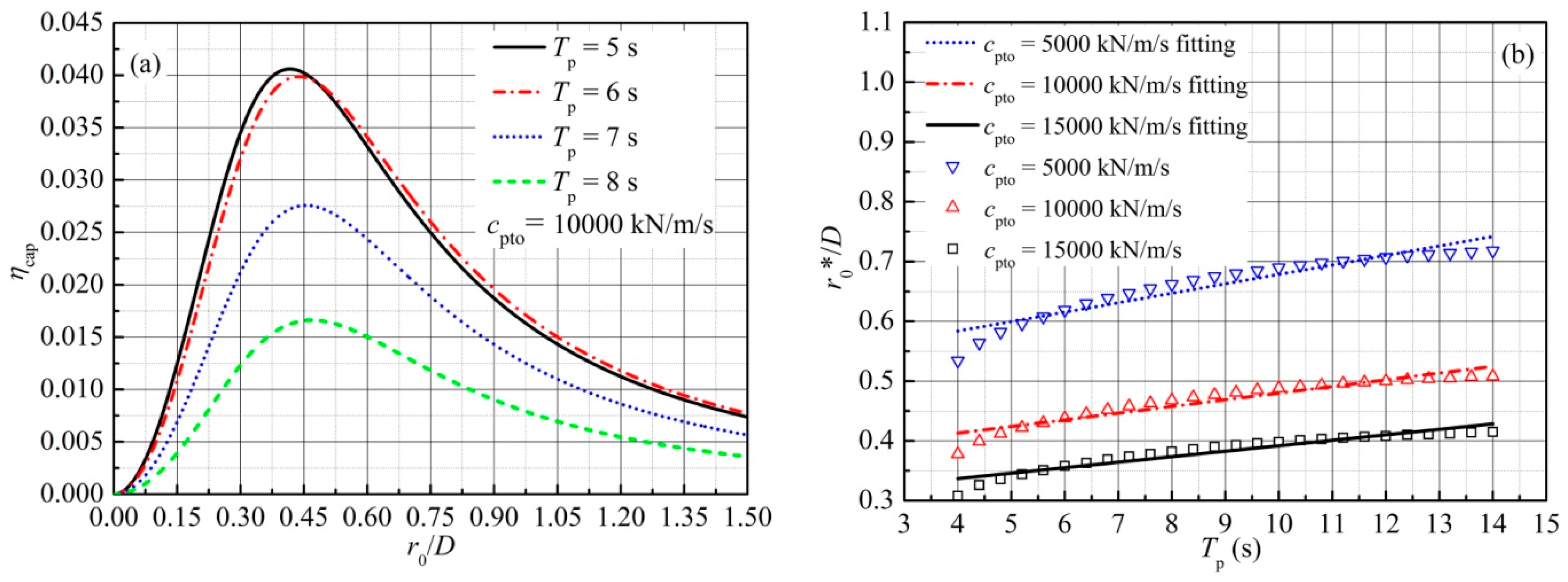
In regular waves, it is found that there exists an optimal normalized mounting position r0*/D, and the optimal normalized mounting position r0*/D presents an approximately linear relationship with wave period. In this section, we intend to investigate how the capture width ratio varies with mounting position r0 in irregular waves. A wide range of mounting positions r0 are examined. Figure 11a shows the variation of capture width ratio ηcap with normalized mounting position r0/D for the device with a type-four parameter, whereas the variation of the optimal normalized mounting position r0*/D with peak wave period is presented in Figure 11b.
One can see that, similar to the results in regular waves, for a specified peak wave period Tp and a specified damping coefficient cpto, there exists an optimal normalized mounting position r0*/D. However, unlike the results in regular waves, the relationship between the optimal normalized mounting position r0*/D and the peak wave period Tp presents obvious nonlinear characteristics in irregular waves. This is perhaps due to the random nature of the irregular waves.
5.4.2. Influence of Damping Coefficient cpto and Stiffness kpto
As it has been demonstrated that in regular waves the damping coefficient cpto and the stiffness kpto play a significant role in the capture width ratio, we wonder whether the damping coefficient cpto and the stiffness kpto play a similar role in the capture width ratio in irregular waves. Figure 12a,b show the influence of the damping coefficient cpto and stiffness kpto on the capture width ratio of the device with a type-four parameter in irregular waves. Unlike the results in regular waves, it can be seen from Figure 12b that the optimal stiffness kpto* not only depends on the peak wave period but also increases slightly with an increasing damping coefficient cpto, and the optimal damping coefficient cpto* is not symmetric to the optimal stiffness kpto*. The variation of the optimal damping coefficient cpto* and the optimal stiffness kpto* in the optimal combination with peak wave period is presented in Figure 12c. Similar to the results in regular waves, the optimal stiffness kpto* in the optimal combination is negative and decreases with increasing peak wave period, whereas the optimal damping coefficient cpto* in the optimal combination increases with increasing peak wave period, and then decreases after reaching a peak value.
5.4.3. Influence of Surge and Heave Motions of Joint
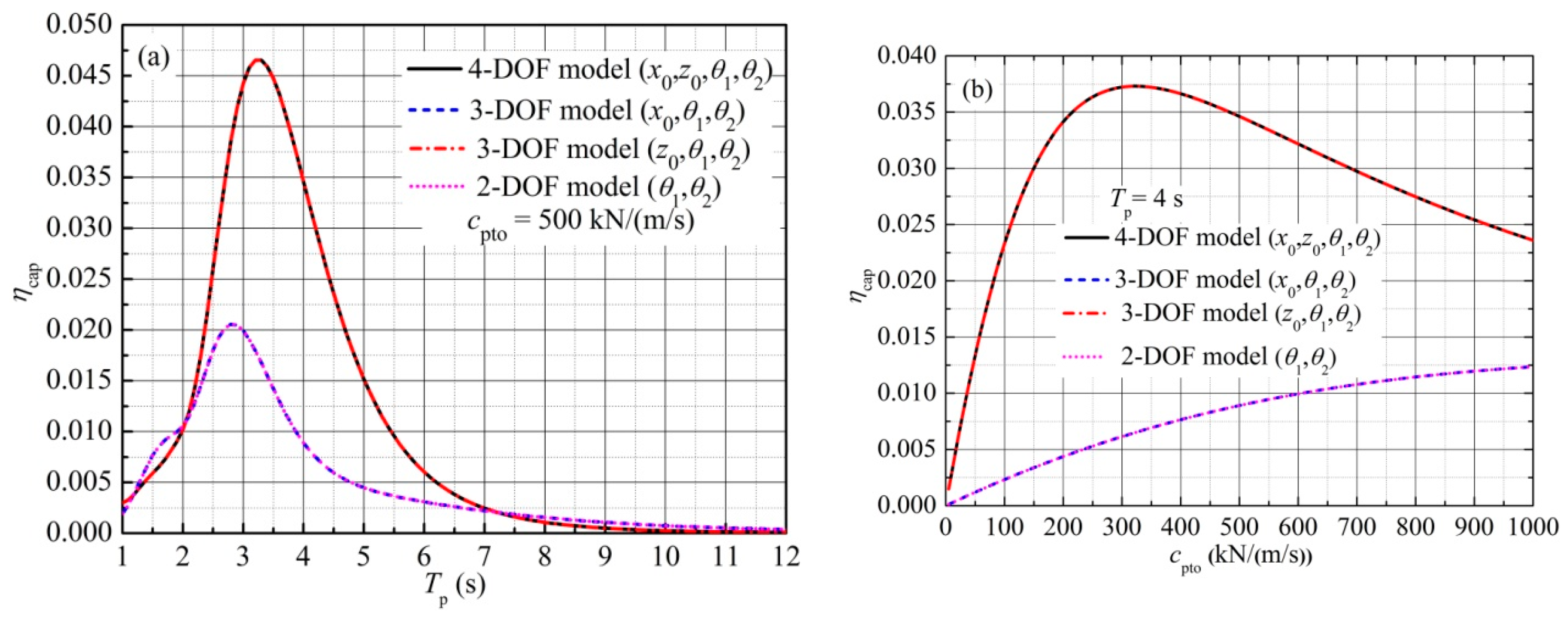
To see whether surge and heave motions of the joint affect the power capture ability of the device in irregular waves, the capture width ratio of the device with a type-one parameter is examined by using the model with and without a consideration of surge and heave motions of the joint. Figure 13a shows the variation of capture width ratio ηcap with peak wave period, whereas the variation of capture width ratio ηcap with damping coefficient cpto is presented in Figure 13b.
Similar to the results in regular waves, it can be seen from Figure 13 that the surge motion of the joint has no effect on the capture width ratio, whereas the heave motion of the joint makes much difference to the capture width ratio.
5.4.4. Influence of Quadratic Damping PTO
As it was demonstrated in the previous section that the peak capture width ratio ηcap* obtained by using quadratic damping is slightly larger than that obtained by using linear damping in regular waves, it is necessary to investigate how quadratic damping β influences the capture width ratio ηcap in irregular waves. Figure 14a shows the variation of capture width ratio ηcap with quadratic damping coefficient β, whereas the variation of peak capture width ratio ηcap* with peak wave period is presented in Figure 14b. As shown in Figure 14a, there exists an optimal quadratic damping coefficient β*, which corresponds to a peak capture width ratio ηcap*. However, unlike the results in regular waves, it can be seen from Figure 14b that the peak capture width ratio ηcap* obtained by using quadratic damping is almost the same as that obtained by using linear damping.
6. Conclusions
In this paper, a state-space approximation of the convolution term in a time domain analysis of a raft-type WEC consisting of two rafts and a PTO unit is presented. The state-space model is identified through regression in the frequency domain. Verification of such a type of time domain analysis is conducted by comparison of its simulation results with those calculated by using frequency domain analysis, and there is a good agreement. The effects of PTO parameters, wave frequency, surge and heave motions of the joint, and quadratic damping PTO on the power capture ability of such a raft-type WEC are investigated. From the above investigations, some conclusions can be drawn as follows:
- (1)
- State-space approximation of the convolution term through regression in the frequency domain has sufficient accuracy. The time domain analysis with the convolution term approximated by a state-space model could be used to investigate the performance of the device.
- (2)
- To obtain a relatively large capture width ratio, the resonant frequency of the designed device should be as close to the considered wave frequency as possible. When there is no control included in the PTO unit, the arrival of resonance is usually at the cost of a relatively large raft size.
- (3)
- For a certain wave period (or peak wave period), there exists an optimal mounting position r0*, corresponding to a peak capture width ratio ηcap*. In regular waves, the relationship between the optimal normalized mounting position r0*/D and the wave period is approximately linear, and a smaller damping coefficient cpto gives a larger gradient of the approximately linear relationship; however, this relationship presents nonlinear characteristics in irregular waves.
- (4)
- In regular waves, the optimal stiffness kpto* only depends on wave period, and the optimal damping coefficient cpto* relies on wave period and stiffness kpto, and is symmetric to the optimal stiffness kpto*. However, in irregular waves, the optimal stiffness kpto* depends on not only the wave period, but also the damping coefficient cpto, and the optimal damping coefficient cpto* is not symmetric to the optimal stiffness kpto*. The optimal damping coefficient cpto* in the optimal combination increases with increasing wave period (or peak wave period), and then decreases after reaching a peak value, whereas the optimal stiffness kpto* in the optimal combination is usually negative and decreases monotonously.
- (5)
- The surge motion of the joint could be neglected. The motion equation of the device can be reduced to a three-DOF model only with the consideration of heave motion of the joint and two pitch motions of the two rafts.
- (6)
- In regular waves, the peak capture width ratio ηcap* obtained by using quadratic damping is slightly larger than that obtained by using linear damping; however, this advantage vanishes in irregular waves.
The present model based on potential theory is relatively convenient to predict the performance of the raft-type WEC. However, without any consideration of energy dissipation due to the fluid viscosity, vortex shedding, and turbulence, it may over-assess the captured power and consequently leads to an over-estimation of the capture width ratio. This problem will be studied in the near future.
Acknowledgments
The authors gratefully acknowledge the support of National Natural Science Foundation of China (51075081).
Author Contributions
Changhai Liu derived the model, performed the simulation, and wrote the paper; Qingjun Yang was responsible for supervising this research and was involved in exchanging ideas and reviewing the article draft; Gang Bao contributed analysis methods.
Conflicts of Interest
The authors declare no conflict of interest.
Appendix A
Here, m is the mass of each raft; Ic is the rotary inertia about the centre of mass; auj and buj are the frequency-dependent added mass and radiation damping at mode u due to the motion of mode j (u = 1, 3, 5, 1′, 3′, 5′; j = 1, 3, 5, 1′, 3′, 5′), respectively; k33 and k3′3′ are the hydrostatic restoring stiffnesses of the fore and aft rafts caused by the their heave motions, respectively; k55 and k5′5′ are the hydrostatic restoring stiffnesses of the fore and aft rafts caused by the their pitch motions, respectively; Γj (ω) is the complex excitation force coefficient at mode j (force per unit incident wave amplitude); the modulus and argument of Γj (ω) are |Γj (ω)| and ∠Γj (ω), respectively; r0 is half the distance of the mounting position between the top and bottom hydraulic cylinders, as shown in Figure 1b; and cpto and kpto are the equivalent damping coefficient and stiffness of the hydraulic cylinder, respectively.
Formulations for resembling the total state-space model:
References
- McCormick, M.E. Ocean Wave Energy Conversion; Dover Publications: Mineola, NY, USA, 2007; Volume 45, ISBN 9780486462455. [Google Scholar]
- Cruz, J. Ocean Wave Energy-Current Status and Future Prespectives; Springer Science & Business Media: Berlin, Germany, 2008; ISBN 978-3-540-74894-6. [Google Scholar]
- Drew, B.; Plummer, A.R.; Sahinkaya, M.N. A review of wave energy converter technology. Proc. Inst. Mech. Eng. Part A J. Power Energy 2009, 223, 887–902. [Google Scholar] [CrossRef]
- López, I.; Andreu, J.; Ceballos, S.; de Alegría, I.M.; Kortabarria, I. Review of wave energy technologies and the necessary power-equipment. Renew. Sustain. Energy Rev. 2013, 27, 413–434. [Google Scholar] [CrossRef]
- Haren, P. Optimal Design of Hagen-Cockerell Raft. Master’s Thesis, Massachusetts Institute of Technology, Cambridge, MA, USA, 1979. [Google Scholar]
- Haren, P.; Mei, C.C. Head-sea diffraction by a slender raft with application to wave-power absorption. J. Fluid Mech. 1981, 104, 505–526. [Google Scholar] [CrossRef]
- Haren, P.; Mei, C.C. An array of Hagen-Cockerell wave power absorbers in head seas. Appl. Ocean Res. 1982, 4, 51–56. [Google Scholar] [CrossRef]
- Haren, P.; Mei, C.C. Wave power extraction by a train of rafts: Hydro-dynamic theory and optimum design. Appl. Ocean Res. 1979, 1, 147–157. [Google Scholar] [CrossRef]
- Farley, F.J.M. Wave energy conversion by flexible resonant rafts. Appl. Ocean Res. 1982, 4, 57–63. [Google Scholar] [CrossRef]
- Kraemer, D.R.B. The Motions of Hinged-Barge Systems in Regular Seas. Ph.D. Thesis, Johns Hopkins University, Baltimore, MD, USA, 2001. [Google Scholar]
- Nolan, G.; Catháin, M.; Murtagh, J.; Ringwood, J. Modelling and Simulation of the Power Take-Off System for a Hinge-Barge Wave-Energy Converter. In Proceedings of the Fifth European Wave Energy Conference, University College Cork, Ireland, 17–20 September 2003; pp. 1–8. [Google Scholar]
- Paparella, F.; Bacelli, G.; Paulmeno, A.; Mouring, S.E.; Ringwood, J.V. Multibody Modelling of Wave Energy Converters Using Pseudo-Spectral Methods with Application to a Three-Body Hinge-Barge Device. IEEE Trans. Sustain. Energy 2016, 7, 966–974. [Google Scholar] [CrossRef]
- Retzler, C. Measurements of the slow drift dynamics of a model Pelamis wave energy converter. Renew. Energy 2006, 31, 257–269. [Google Scholar] [CrossRef]
- Yemm, R.; Pizer, D.; Retzler, C.; Henderson, R. Pelamis: Experience from concept to connection. Philos. Trans. R. Soc. A Math. Phys. Eng. Sci. 2012, 370, 365–380. [Google Scholar] [CrossRef] [PubMed]
- Henderson, R. Design, simulation, and testing of a novel hydraulic power take-off system for the Pelamis wave energy converter. Renew. Energy 2006, 31, 271–283. [Google Scholar] [CrossRef]
- Thiam, A.G.; Pierce, A.D. Segmented and continuous beam models for the capture of ocean wave energy by Pelamis-like devices. Proc. Meet. Acoust. 2012, 11, 65001. [Google Scholar] [CrossRef]
- Thiam, A.G.; Pierce, A.D. Radiation loss in Pelamis-like ocean wave energy conversion devices. Proc. Meet. Acoust. 2013, 12, 65003. [Google Scholar] [CrossRef]
- Thiam, A.G.; Pierce, A.D. Damping mechanism concepts in ocean wave energy conversion: A simplified model of the Pelamis converter. J. Acoust. Soc. Am. 2010, 127, 65002. [Google Scholar] [CrossRef]
- Zheng, S.; Zhang, Y.; Sheng, W. Maximum theoretical power absorption of connected floating bodies under motion constraints. Appl. Ocean Res. 2016, 58, 95–103. [Google Scholar] [CrossRef]
- Zheng, S.-M.; Zhang, Y.-H.; Zhang, Y.-L.; Sheng, W.-A. Numerical study on the dynamics of a two-raft wave energy conversion device. J. Fluids Struct. 2015, 58, 271–290. [Google Scholar] [CrossRef]
- Sun, L.; Taylor, R.E.; Choo, Y.S. Responses of interconnected floating bodies. IES J. Part A Civ. Struct. Eng. 2011, 4, 143–156. [Google Scholar] [CrossRef] [Green Version]
- Sun, L.; Stansby, P.; Zang, J.; Moreno, E.C.; Taylor, P.H. Linear diffraction analysis for optimisation of the three-float multi-mode wave energy converter M4 in regular waves including small arrays. J. Ocean Eng. Mar. Energy 2016, 2, 429–438. [Google Scholar] [CrossRef]
- Sun, L.; Zang, J.; Stansby, P.; Moreno, E.C.; Taylor, P.H.; Taylor, R.E. Linear diffraction analysis of the three-float multi-mode wave energy converter M4 for power capture and structural analysis in irregular waves with experimental validation. J. Ocean Eng. Mar. Energy 2017, 3, 51–68. [Google Scholar] [CrossRef]
- Stansby, P.; Moreno, E.C.; Stallard, T. Large capacity multi-float configurations for the wave energy converter M4 using a time-domain linear diffraction model. Appl. Ocean Res. 2017, 68, 53–64. [Google Scholar] [CrossRef]
- Taghipour, R.; Perez, T.; Moan, T. Hybrid frequency-time domain models for dynamic response analysis of marine structures. Ocean Eng. 2008, 35, 685–705. [Google Scholar] [CrossRef]
- Kristiansen, E.; Hjulstad, Å.; Egeland, O. State-space representation of radiation forces in time-domain vessel models. Model. Identif. Control 2006, 27, 23–41. [Google Scholar] [CrossRef]
- Liu, C.; Yang, Q.; Bao, G. Performance investigation of a two-raft-type wave energy converter with hydraulic power take-off unit. Appl. Ocean Res. 2017, 62, 139–155. [Google Scholar] [CrossRef]
- Falnes, J. Ocean Waves and Oscillating Systems: Linear Interactions Including Wave-Energy Extraction; Cambridge University Press: Cambridge, UK, 2002; Volume 56, ISBN 0521017491. [Google Scholar]
- Newman, J.N. Absorption of wave energy by elongated bodies. Appl. Ocean Res. 1979, 1, 189–196. [Google Scholar] [CrossRef]
- Taghipour, R.; Perez, T.; Moan, T. Time-Domain Hydroelastic Analysis of a Flexible Marine Structure Using State-Space Models. J. Offshore Mech. Arct. Eng. 2008, 131, 11603. [Google Scholar] [CrossRef]
- Perez, T.; Fossen, T.I. Practical aspects of frequency-domain identification of dynamic models of marine structures from hydrodynamic data. Ocean Eng. 2011, 38, 426–435. [Google Scholar] [CrossRef]
- Duarte, T.; Sarmento, A.; Alves, M.; Jonkman, J. State-Space Realization of the Wave-Radiation Force within FAST. In Proceedings of the ASME 32nd International Conference on Ocean, Offshore and Arctic Engineering, Nantes, France, 9–14 June 2013; pp. 1–12. [Google Scholar] [CrossRef]
- Sanathanan, C.; Koerner, J. Transfer function synthesis as a ratio of two complex polynomials. IEEE Trans. Automat. Contr. 1963, 8, 56–58. [Google Scholar] [CrossRef]
- ANSYS AQWA. Available online: http://www.ansys.com/fr-fr/products/structures/ansys-aqwa (accessed on June 2015).
- Wang, D.; Qiu, S.; Ye, J. An experimental study on a trapezoidal pendulum wave energy converter in regular waves. China Ocean Eng. 2015, 29, 623–632. [Google Scholar] [CrossRef]
- Faltinsen, O.M. Sea Loads on Ships and Offshore Structures; Cambridge University Press: Cambridge, UK, 1990; Volume 1, ISBN 0-521-45870-6. [Google Scholar]
Figure 1.
Schematic of a raft-type WEC consisting of two rafts and a PTO unit: (a) Front view (b) Initial position and (c) Position after motion.
Figure 1.
Schematic of a raft-type WEC consisting of two rafts and a PTO unit: (a) Front view (b) Initial position and (c) Position after motion.

Figure 2.
General idea of assembling the state-space model.

Figure 3.
Identification results of retardation functions: (a) H11 (−iω); (b) H13 (−iω); (c) H22 (−iω); (d) H23 (−iω); (e) H33 (−iω); (f) H34 (−iω).
Figure 3.
Identification results of retardation functions: (a) H11 (−iω); (b) H13 (−iω); (c) H22 (−iω); (d) H23 (−iω); (e) H33 (−iω); (f) H34 (−iω).

Figure 4.
Performance of the device in regular waves (FD = Frequency domain TD = Time domain): (a) Amplitude of Gv_rp; (b) Pave_cap; and (c) ηcap.
Figure 4.
Performance of the device in regular waves (FD = Frequency domain TD = Time domain): (a) Amplitude of Gv_rp; (b) Pave_cap; and (c) ηcap.

Figure 5.
Influence of wave frequency in regular waves (FD = Frequency domain TD = Time domain): (a) Pave_cap; and (b) ηcap.
Figure 5.
Influence of wave frequency in regular waves (FD = Frequency domain TD = Time domain): (a) Pave_cap; and (b) ηcap.

Figure 6.
Influence of mounting position in regular waves: (a) Variation of ηcap with r0/D; and (b) Variation of r0*/D with T.
Figure 6.
Influence of mounting position in regular waves: (a) Variation of ηcap with r0/D; and (b) Variation of r0*/D with T.

Figure 7.
Influence of damping coefficient and stiffness in regular waves: (a) 3D ηcap in T = 6 s; (b) ηcap contour in T = 6 s; and (c) Optimal damping coefficient and optimal stiffness in optimal combination.
Figure 7.
Influence of damping coefficient and stiffness in regular waves: (a) 3D ηcap in T = 6 s; (b) ηcap contour in T = 6 s; and (c) Optimal damping coefficient and optimal stiffness in optimal combination.

Figure 8.
Influence of surge and heave motions of joint in regular waves: (a) Variation of Amplitude of Gv_rp with kL; (b) Variation of ηcap with kL; and (c) Variation of ηcap with cpto.
Figure 8.
Influence of surge and heave motions of joint in regular waves: (a) Variation of Amplitude of Gv_rp with kL; (b) Variation of ηcap with kL; and (c) Variation of ηcap with cpto.

Figure 9.
Performance of the device with quadratic damping PTO in regular waves: (a) Variation of and fθ1(t) with time; and (b) Variation of ηcap with β.
Figure 9.
Performance of the device with quadratic damping PTO in regular waves: (a) Variation of and fθ1(t) with time; and (b) Variation of ηcap with β.

Figure 10.
Variation of ηcap* with wave period for the device with linear damping or quadratic damping.
Figure 10.
Variation of ηcap* with wave period for the device with linear damping or quadratic damping.

Figure 11.
Influence of mounting position in irregular waves: (a) Variation of ηcap with r0/D; and (b) Variation of r0*/D with Tp.
Figure 11.
Influence of mounting position in irregular waves: (a) Variation of ηcap with r0/D; and (b) Variation of r0*/D with Tp.

Figure 12.
Influence of damping coefficient and stiffness in irregular waves: (a) 3D ηcap in Tp = 6 s; (b) ηcap contour in Tp = 6 s; and (c) Optimal damping coefficient and optimal stiffness in optimal combination.
Figure 12.
Influence of damping coefficient and stiffness in irregular waves: (a) 3D ηcap in Tp = 6 s; (b) ηcap contour in Tp = 6 s; and (c) Optimal damping coefficient and optimal stiffness in optimal combination.
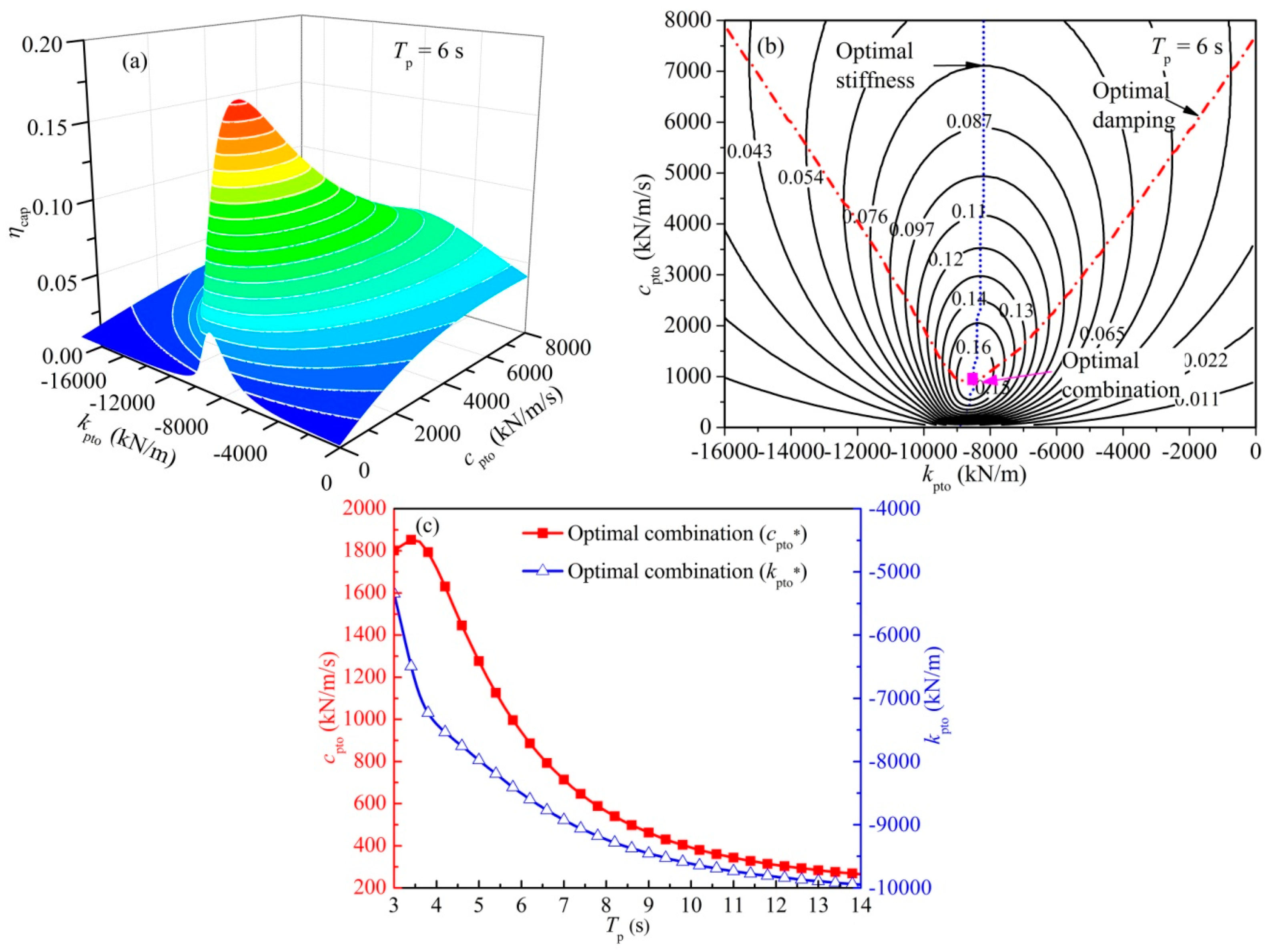
Figure 13.
Influence of surge and heave motions of joint in irregular waves: (a) Variation of ηcap with Tp; and (b) Variation of ηcap with cpto.
Figure 13.
Influence of surge and heave motions of joint in irregular waves: (a) Variation of ηcap with Tp; and (b) Variation of ηcap with cpto.

Figure 14.
Influence of quadratic damping PTO in irregular waves: (a) Variation of ηcap with β; and (b) Variation of ηcap* with Tp.
Figure 14.
Influence of quadratic damping PTO in irregular waves: (a) Variation of ηcap with β; and (b) Variation of ηcap* with Tp.


Table 1.
Four types of parameters.
| Parameter | Type-One | Type-Two | Type-Three | Type-Four |
|---|---|---|---|---|
| Raft length L (m) | 10 | 20 | 20 | 30 |
| Raft diameter D (m) | 1 | 1 | 2 | 2 |
| Raft space d0 (m) | 1 | 1 | 1 | 1 |
| Raft density ρ0 (kg/m3) | 512.5 | 512.5 | 512.5 | 512.5 |
| Raft volume V/m3 | 7.8540 | 15.7080 | 62.8319 | 94.2478 |
| Damping coefficient cpto (kN/m/s) | 500 | 500 | 500 | 500 |
| Mounting position r0 (m) | 0.5 | 0.5 | 1 | 1 |
| Optimal ratio kL | 3.1163 | 3.6184 | 3.4987 | 3.6715 |
| Optimal ratio of raft length to wavelength | 0.4960 | 0.5759 | 0.5568 | 0.5843 |
| Resonant frequency of relative pitch velocity ωrp (rad/s) | 1.7485 | 1.3322 | 1.3100 | 1.0957 |
| Resonant frequency of heave velocity ωh (rad/s) | 1.4078 | 1.2354 | 1.2100 | 1.0179 |
| Resonant frequency of surge velocity ωs (rad/s) | 1.0144 | 0.7370 | 0.7322 | 0.6021 |
| Amplitude of FRF of wave amplitude to relative pitch velocity at ωrp (rad/s/m) | 0.4281 | 0.3181 | 0.3054 | 0.1799 |
| Amplitude of FRF of wave amplitude to heave velocity at ωh (m/s/m) | 1.2623 | 1.5099 | 1.4735 | 1.2589 |
| Amplitude of FRF of wave amplitude to surge velocity at ωs (m/s/m) | 0.7881 | 0.5624 | 0.5655 | 0.4674 |
© 2018 by the authors. Licensee MDPI, Basel, Switzerland. This article is an open access article distributed under the terms and conditions of the Creative Commons Attribution (CC BY) license (http://creativecommons.org/licenses/by/4.0/).
Share and Cite
MDPI and ACS Style
Liu, C.; Yang, Q.; Bao, G. State-Space Approximation of Convolution Term in Time Domain Analysis of a Raft-Type Wave Energy Converter. Energies 2018, 11, 169. https://doi.org/10.3390/en11010169
AMA Style
Liu C, Yang Q, Bao G. State-Space Approximation of Convolution Term in Time Domain Analysis of a Raft-Type Wave Energy Converter. Energies. 2018; 11(1):169. https://doi.org/10.3390/en11010169
Chicago/Turabian StyleLiu, Changhai, Qingjun Yang, and Gang Bao. 2018. "State-Space Approximation of Convolution Term in Time Domain Analysis of a Raft-Type Wave Energy Converter" Energies 11, no. 1: 169. https://doi.org/10.3390/en11010169
Note that from the first issue of 2016, this journal uses article numbers instead of page numbers. See further details here.