Impact on Congestion and Fuel Consumption of a Cooperative Adaptive Cruise Control System with Lane-Level Position Estimation

Abstract

In recent years, vehicular communications systems have evolved and allowed for the improvement of adaptive cruise control (ACC) systems to make them cooperative (cooperative adaptive cruise control, CACC). Conventional ACC systems use sensors on the ego-vehicle, such as radar or computer vision, to generate their behavioral decisions. However, by having vehicle-to-X (V2X) onboard communications, the need to incorporate perception in the vehicle is drastically reduced. Thus, in this paper a CACC solution is proposed that only uses communications to make its decisions with the help of previous road mapping. At the same time, a method to develop these maps is presented, combining the information of a computer vision system to correct the positions obtained from the navigation system. In addition, the cut-in and cut-out maneuvers for a CACC platoon are taken into account, showing the tests of these situations in real environments with instrumented vehicles. To show the potential of the system in a larger-scale implementation, simulations of the behavior are provided under dense traffic conditions where the positive impact on the reduction of traffic congestion and fuel consumption is appreciated.

1. Introduction

Technological advances in the last years have improved the precision of geolocalization systems [1] while reducing their costs. This has allowed the data obtained from geographical positioning systems to be implemented more efficiently in the automotive field. With better precision of global navigation satellite systems (GNSSs), [2] geographic positioning system (GPS) data can be entered into a global information system (GIS) database.

With a database built from the retrieved geographical positions, the next step is the development of digital road maps, but in order to do so, accuracy needs to be improved, as the inherent error of the GNSS receptors oscillates between 1 and 10 m. For enhancing such accuracy, there already exist algorithms such as Hao Wu’s [3] which allow precision improvements of GNSS receptors of up to 90%.

Other algorithms allow precision enhancement of GNSS in real time, such as Tao’s method [4], depicting corrections of obtained data of the GNSS using computer vision. Another possibility is presented in [5] where a map is made implementing both GPS and inertial sensors to obtain accurate maps. If these technologies are combined, a really accurate digital map can be made, including the identification of different lanes.

On the other hand, in recent years, vehicle-to-X (V2X) communications have begun to take relevance in automotion, allowing data sharing between different vehicles and/or other entities, like infrastructures. These communications enable information exchange among the elements of the network, overcoming the limitation of the visual horizon of the ego-vehicle when receiving information from its surroundings. Nowadays, these communications are standardized by the IEEE 802.11p or ETSI EN-306 [6,7]. However, the tendency is to hybridize these communications with systems based on mobile telephony.

V2X communications make possible the deployment of cooperative intelligent transport systems (C-ITSs), defined as ‘a subset of the overall ITS that communicates and shares information between ITS stations to give advice or facilitate actions with the objective e of improving safety, sustainability, efficiency and comfort beyond the scope of stand-alone systems’ [8].

C-ITS applications are organized as Day-1 and Day-2 [8] according to proximity of their implantation, and a great number of applications that make use of the advantages of vehicular communications systems have been proposed. One of the most classic ones is truck platooning, as in [9]. The authors resolve the interference produced by other vehicles by implementing several emission antennas on each vehicle.

Cooperative systems have been used as an upgrade of advanced driver assistance systems (ADASs). In this sense, adaptive cruise control (ACC) has evolved to cooperative adaptive cruise control (CACC) that sets the cruise control for the vehicle that uses the information obtained via communications systems to make decisions.

Schmied [10] proposes a CACC system with vehicle to infrastructure (V2I) communications that is capable of reducing the vehicle’s consumption and therefore, its emissions. Other example of CACC with several vehicles is posed by Shladover [11] where the system is tested under real traffic conditions in order to cooperate with other vehicles, regardless of whether communications modules were installed.

More references available on CACC systems [12,13] contribute with solutions to different problems occurring in certain situations and in [14] a review of CACC systems and the different developed algorithms is presented, exposing the highlights of each.

The impact of these technologies in traffic is hard to measure. In one hand, traffic is an environment tied to highly strict safety regulations that hinder instrumentation and monitoring activities. On the other hand, it behaves as a complex system which arises from the interaction of a great number of individual elements and whose evolution is highly sensitive to initial conditions. Furthermore, currently there are not enough connected vehicles to evaluate the implantation on the field. This is why an ideal way to measure the performance is by means of simulators that allow realist studies of massive implantation of these kinds of C-ITSs.

An example of the impact of CACC and ACC systems over traffic density is presented by Delis [15,16] that shows that if only 20% of the vehicles were to use an ACC system, the traffic congestion would be substantially reduced. In addition, in [17] show that savings in the consumption of heavy vehicles can be reduced by 20% by coordinating driving with platooning systems. Using a macroscopic simulation tool, the traffic density evolution is predicted with both an ACC system and a CACC one. However, being a macroscopic simulation, the functional aspects of the C-ITS applications are not taken into account, such as positioning accuracy or the trust level when detecting the driving lane.

In this paper, a CACC system is presented that only uses the data received by V2X communications with GPS navigation devices without recurring to other environment supervision systems. The communications allow for platooning behavior and speed control, and additionally this article shows the possibilities of realizing and detecting lane changes. To prove all these functionalities and real capabilities, the system has been tested on real environments. Furthermore, to complete the test, simulations of the system behavior at a macroscopic level were also made, analyzing the impact in traffic density from the interaction of vehicles as entities with or without CACC, thus offering a more realistic vision of a large-scale deployment.

2. Methodology and System Description

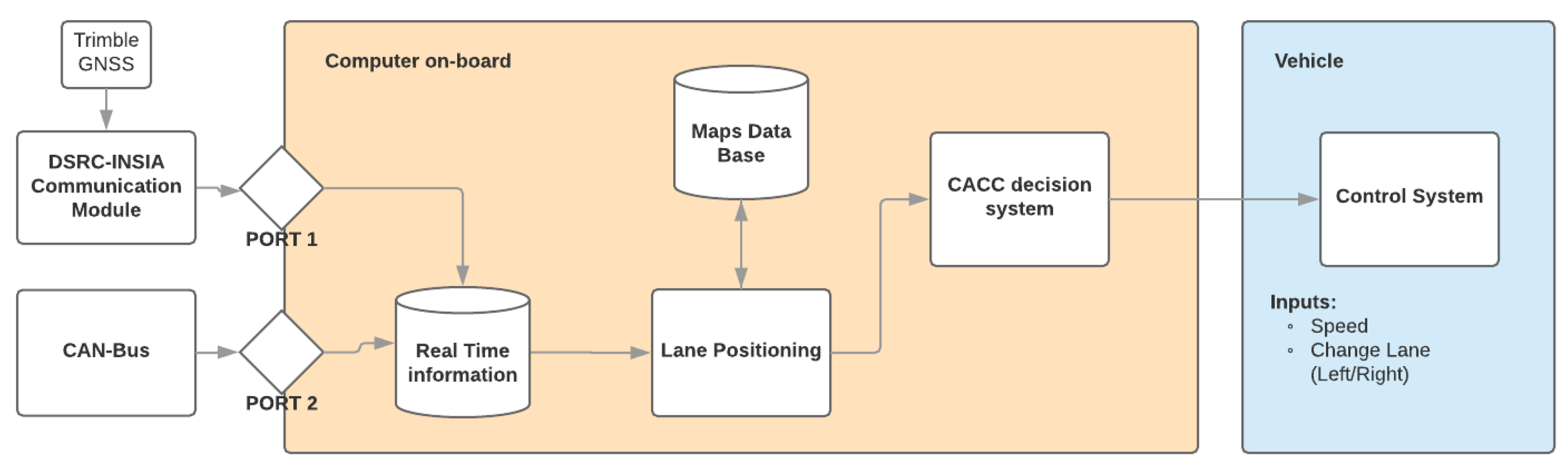
The designed system bases its operation on several elements: an accurate digital map at the lane level of the road, a communications system that supports the CACC, and an algorithm of positioning in the lane and decision algorithms of the CACC, designed for the optimal positioning of the vehicle as well as its correct interaction and operability. Figure 1 depicts the relationship between the different components of the CACC system with the vehicle’s control model. The figure is divided into three segments: data collection, a CACC system executed on an on-board computer, and a vehicle control system. In the data collection segment, using the communications module DSRC-INSIA (Dedicated Short Range Communication) and CAN-Bus, the geographical positions of all the vehicles that have modules and the local vehicle speed are obtained. With this information only, lane positioning for each vehicle cannot be performed, so a digital map of the roads and a lane positioning algorithm allowing each vehicle to be placed in a specific lane have been developed. Once each vehicle has been positioned, the CACC system can make decisions about the speed or lane change to be sent to the control system. The algorithm works locally in each vehicle, which means that it only uses the information received from communications; no message is sent to the rest of the vehicles.

In this way, the CACC system is subsequently allowed to make decisions on distance adaptation or lane change. For this, it is necessary to use geopositioning of the different vehicles of the network in each lane using a specific algorithm for the precise discrimination of the lane. Then, the responses of the lane or speed changes generated by the system are adapted according to traffic conditions.

The following sections explain the algorithms, as well as the steps that have been followed for their implementation.

2.1. Development of the Digital Map

The first step is to determine the specifications and actions that have been carried out for the creation of the road database. In order to obtain a more accurate mapping, computer vision tools and GNSS systems with satellite-based augmentation system (SBAS) support have been used with the European Geostationary Navigation Overlay Service (EGNOS). In this way, attempts are made to reduce errors that other methods introduce because of being dependent on the specific trajectory described by the instrumented vehicle [5].

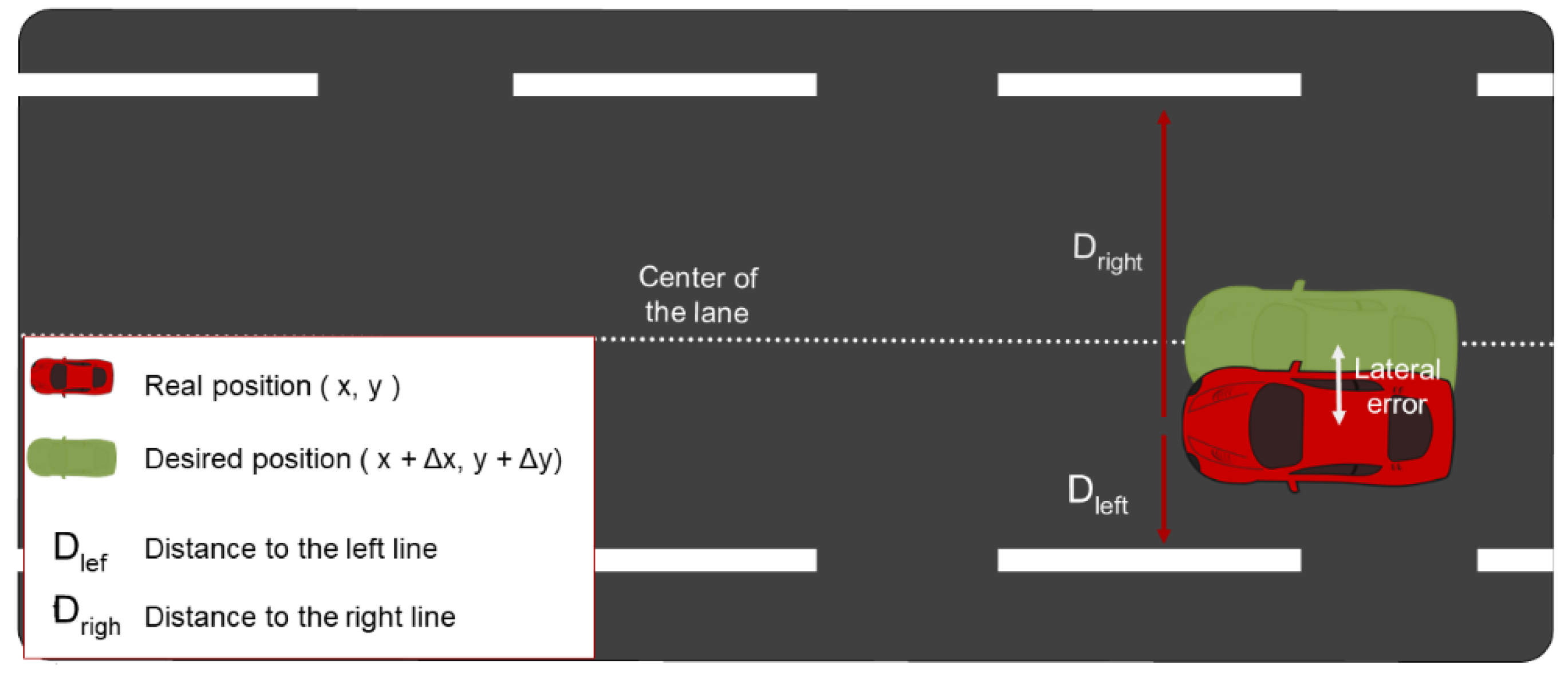
Geographical position data has been obtained using a Trimble R4 GNSS with EGNOS. Additionally, a system based on computer vision Mobileye perception system is used. The computer vision system, located on the central axis of the car, allows for capturing of the distance from the center of the vehicle to the lane lines, the lateral error. The lane width is obtained from the data received from the computer vision system.

In particular, data obtained from the computer vision system allow the GNSS position to be corrected, displacing the geographical positions until reorganizing them in the center of the lane, although the instrumented vehicle has not exactly followed this (Figure 2). This step is carried out to correct the different maneuvers a driver takes and therefore, have an influence on the data collected from the GNSS. To ensure proper corrections to locate the positions in the lane center, we use Equation (1) to calculate the exact displacement projection using the vehicle local Universal Transverse Mercator (UTM) coordinates (x, y), where $\Delta x$ and $\Delta y$ represent the error in both the x and the y coordinates, respectively.

$$\begin{gathered} \Delta x=cos\left(\theta \right)·ℰ·{\sigma }_{North} \\ \Delta y=sin\left(\theta \right)·ℰ·{\sigma }_{East} \end{gathered}$$

(1)

The azimuth angle (α) is a crucial element to calculate all necessary lateral control corrections. A more accurate estimation of α can dramatically improve overall system performance. The calculation of θ depends on the lateral error ($ℰ$) value, to enhance the structure following:

For $(ℰ<0)$:

$$\theta =\{\begin{array}{cc} \alpha ,& 0°\le \alpha <90°\\ \alpha -90,& 90°\le \alpha <180°\\ \alpha -180,& 180°\le \alpha <270°\\ \alpha -270,& otherwise \end{array}$$

(2)

For $\left(ℰ\ge 0\right)$:

$$\theta =\{\begin{array}{cc}90-\alpha ,& 0°\le \alpha <90°\\ 180-\alpha ,& 90°\le \alpha <180°\\ 270-\alpha ,& 180°\le \alpha <270°\\ 360-\alpha ,& otherwise \end{array}$$

(3)

As orientation adjustments are required to make the right correction decision (front vehicle direction), both azimuth angle α and correction direction (σ) are to be calculated as the following:

$${\sigma }_{North}=\left\{\begin{array}{l}-1, if 270°>\alpha \ge 90°\\ +1, otherwise \end{array}\right\}$$

(4)

$${\sigma }_{East}=\left\{\begin{array}{c}-1, if \alpha \le 180°\\ +1, otherwise \end{array}\right\}$$

(5)

where UTM coordinates are obtained from the data of the GNSS, and ∆x and ∆y represent the position correction in UTM north and east coordinates, respectively. ${\sigma }_{North}$ and ${\sigma }_{East}$ are the sign corrections that are made according to the vehicle travel direction, and are obtained by calculating the azimuth angle.

As the last part of the GNSS preprocessing data, it is necessary to generate the mapping of all the lanes that constitute the highway. To check which methodology is better for the road mapping, different tests were carried out to compare two different ways of generating it. Firstly, all the GNSS data of each lane were collected individually. On the other hand, an attempt was made to lighten the task by obtaining only the data from the central lane and generating the rest of the lanes by moving the central lane positions. The first method makes the proposed positioning system more problematic because the geographical positions obtained from each lane are not equidistant (even the corrections). Then, if the geographical positions of two adjacent lanes have a shorter distance between them, it is more probable that the system places a vehicle in that wrong lane. Therefore, in this paper the second method is used since it ensures that the positions of all the lanes are equidistant and positioning results in the CACC are improved.

All the obtained and corrected data become part of a database of the road. This database is loaded in memory in 3-km road stretches; this distance was adjusted after performing tests with different stretch lengths and was the greatest distance that could be stored without applying a significant delay. In this way, the search size is limited and the entire process is streamlined. The data loaded in memory must be updated as the vehicles move along the road.

2.2. Communications System

The CACC system obtains information only through the received data from the V2X communications and the CAN-Bus of the vehicle, that is, it does not use laser sensors or computer vision. The communications have been developed entirely in the research group at the Technical University of Madrid, including the hardware and software. In addition, it uses as a reference the maps generated with high precision positioning and map-matching techniques.

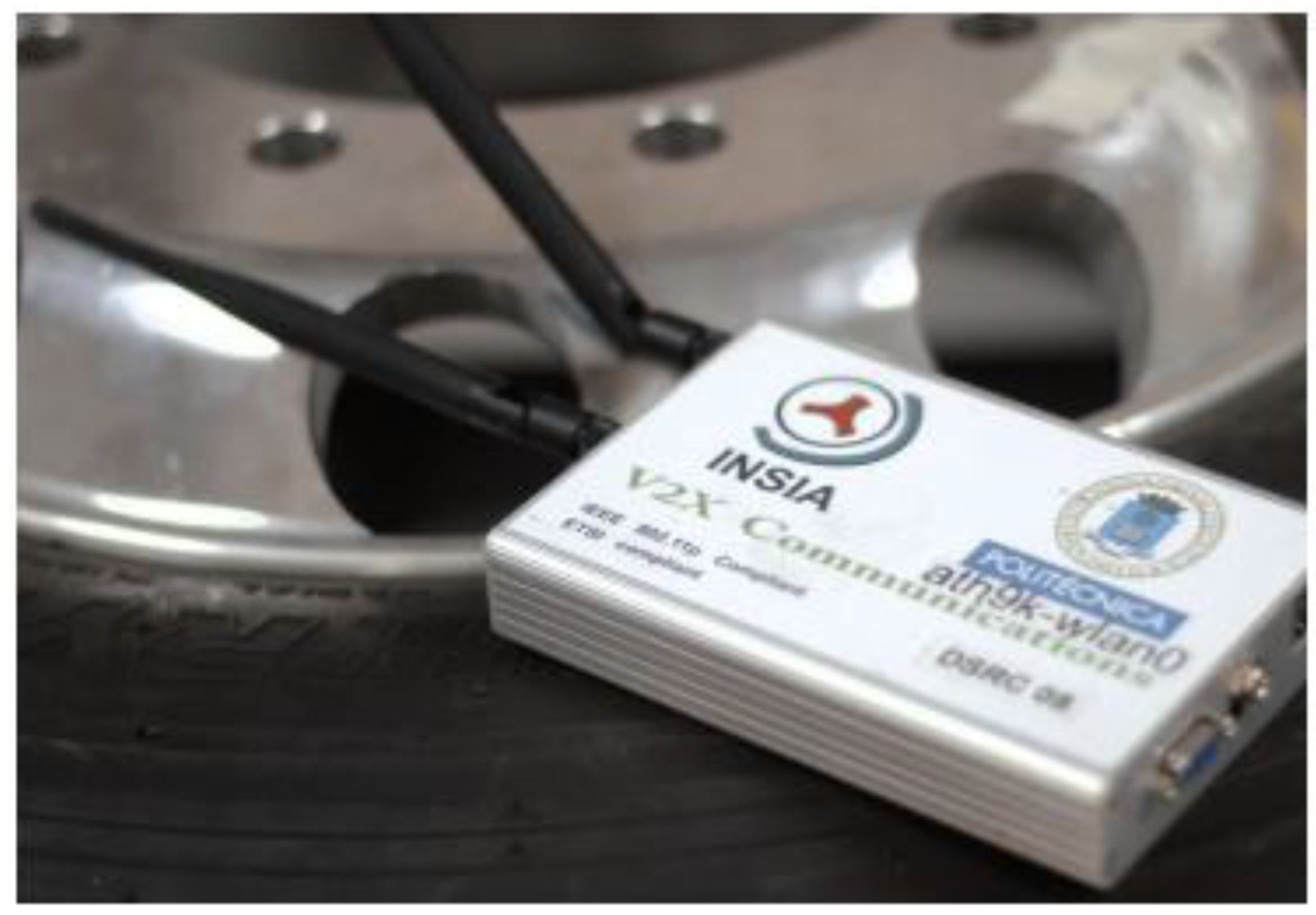
To access the V2X information, the DSRC-INSIA communications module (Figure 1) is used, which is responsible for following the communication protocols between vehicles, as described in [6].

2.3. Estimation of the Driving Lane

The proposed CACC system is based on a precise knowledge of the lane in which the vehicle is moving, making use of the digital map previously obtained. However, due to multiple factors, including positioning systems errors [18], the behavior of the drivers, and the imperfections of the road, this knowledge was not trivial. To obtain the lane through which each vehicle moves, the algorithm uses the data previously stored with the road mapping (Section 2.1). All the tests were carried out in a Skylake Intel I7 6500U, with 8 G RAM. Figure 2 and Figure 3 show operating examples of two different algorithms that allow calculating the lane according to the position of the car.

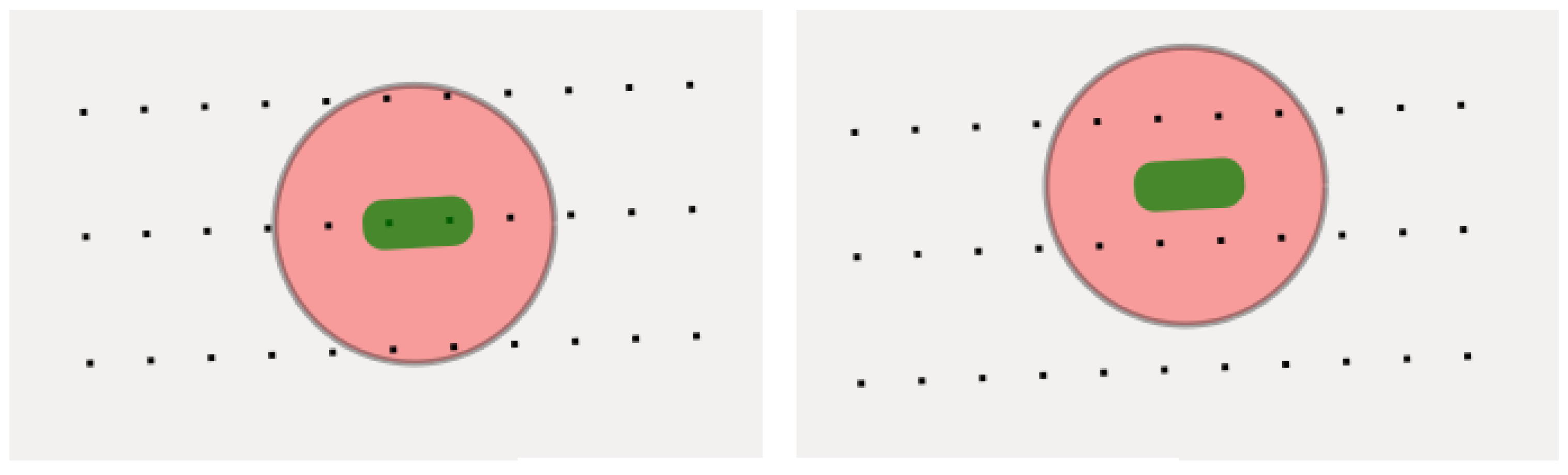
In Figure 4 and Figure 5, the idea of the functioning of each algorithm is represented. The vehicle is represented by a rectangle in green and the center lines of each lane are black-dotted. In the first case (Figure 4), the circumference around the vehicle is calculated and its dimensions are adjustable depending on the width of the lanes.

This algorithm can be interpreted as a mathematical problem of mode calculation obtaining a response with low delay (~45 ms). In the tests carried out the algorithm manages to obtain the lane through which the vehicle drives with an accuracy of 87%. This accuracy is calculated using the algorithm in each data received from the communications module (10 Hz) in a 6-km road stretch in which the lane through which the vehicle moves is known at each moment. This method has problems in situations where the same number of points in one lane are obtained as in another (Figure 4b), which can be due to a lane change but also a deviation in the navigation system data given the uncertainty of this positioning system.

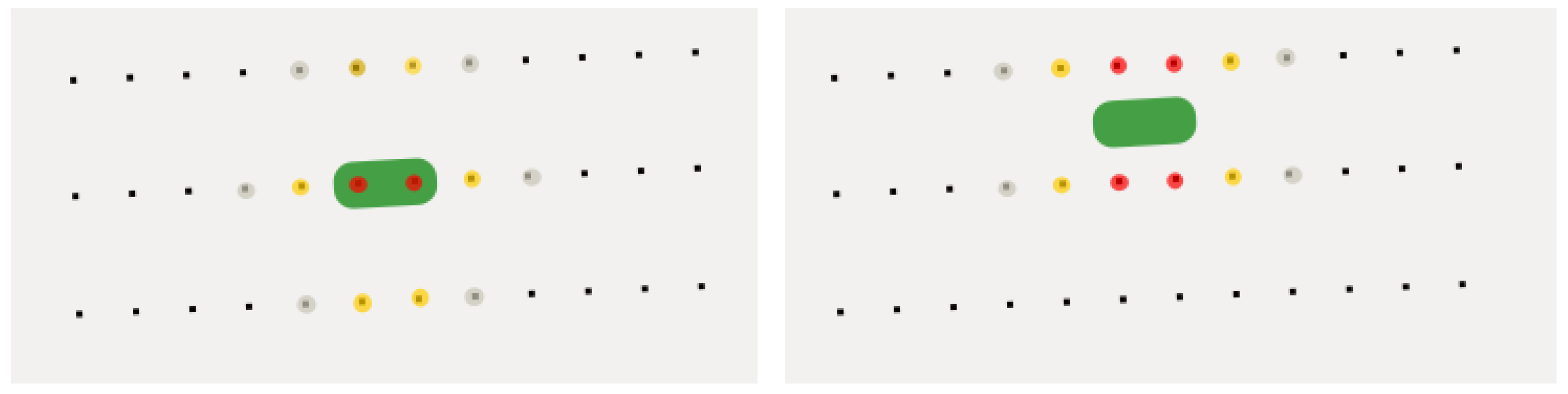
Due to the problems presented by the previous algorithm, it was decided to use the k-nearest neighbors (k-NN) algorithm, where the nearest k nodes are located and thus the degree of belonging to each lane was obtained (Figure 5). In this case, it is a problem of resolving distances with geographical positions using the equation of Euclidean distances (Equation (6)), where the position values correspond to the geographical points of the road ($x_i$, $y_i$) and the latest position of the vehicle ($x_v$, $y_v$). Equation (6) calculates the Euclidean distance with respect of all the points of the sector of 3 km of road that is loaded in memory. The road sector is constantly updated with a double buffer to speed up the process.

$$K_{NN}=\underset{i=0\to n}{\min }\left(\sqrt{{\left(x_v-x_i\right)}^2+{\left(y_v-y_i\right)}^2}\right)$$

(6)

Performing the same positioning tests on both algorithms, the k-NN algorithm obtained the best results, with an accuracy around 90% and a delay of 33 ms. The delay is obtained from the average time used for lane positioning of three vehicles and the fact that including more vehicles in the system does not excessively increase the processing time (3 ms per vehicle).

2.4. CACC Decision Algorithms

Knowing the lane of each vehicle provides new possibilities for performing applications of CACC systems. The purpose of the algorithm is to make decisions on the driving speed, safety distance and, as the most relevant point, the lane-change maneuvers.

Lane-change decisions focus on avoiding accidents and easing traffic congestion on the roads. Therefore, the actions that the CACC system will infer with respect to the car consist in vehicle lane change and adaptation of the same speed with the previous vehicle. This improvement allows for the traffic of a lane to be diverted due to an accident, lane cut, etc.

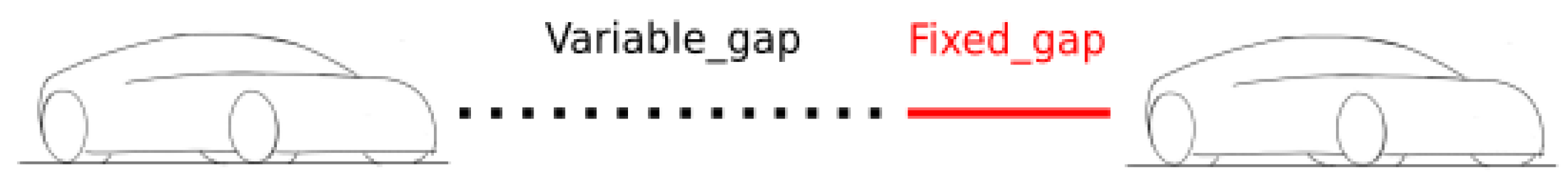
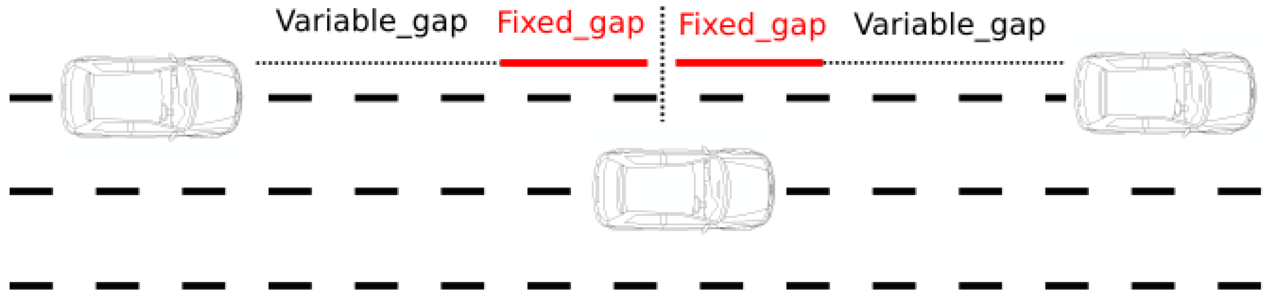
Here we propose a platooning system with cut-in and cut-out maneuvers and lane change maneuvers. In both cases it is important to know the safety distance that the vehicle must maintain at all times. In Figure 6 and Figure 7 a diagram of how the safety distance is calculated is shown. In both cases, it is always necessary to leave a distance that allows driving safely without causing problems to the rest of the road users.

Safety distance consists of a fixed space and a variable one. The fixed space is directly proportional to the error that is obtained in the GNSS systems. The variable space is calculated with the maximum vehicle speeds and the time that there must be between vehicles (~3 s). In [19] a solution is presented to minimize the gap between vehicles with a CACC system, but for this system a gap of 3 s to permit cut-in/cut-out maneuvers is considered, with the possibility of mixed traffic including vehicles with and without communication modules. Furthermore, this approach avoids the need to perform a message delivery system, because the algorithm is oriented to dense traffic situations where it is necessary to avoid saturation of the communication channels.

The final space that must be left to perform the maneuvers or to drive is expressed in Equation (7), where $v_1$ and $v_2$ are the speeds of each vehicle and t represents the time space that should be maintained. In the event that vehicles move at the same speed, a minimum gap is established that will be proportional to the speed.

$$Tota{l}_{gap}=\frac{Max\left(v_1,v_2\right)}{t}+fixedgap$$

(7)

The CACC system must ensure at every moment that safety distances are maintained. To calculate the vehicle speed setpoint, this distance is taken into account and modified in real time to adapt to each situation. A detailed description of the algorithm used to adapt the vehicle speed is shown in [20,21], where the error produced between the real and optimal distance is minimized to keep a safety space.

Finally, it must be taken into account that the safety distance in a lane change must be maintained not only with the vehicle that runs in front of it but also with those that drive behind. When the system wants to make a lane change it locates the vehicles that are in the lane and calculates the distance that separates them. If it is guaranteed that there is no risk of collision with another vehicle and the safety distance is maintained, the lane change instruction will be sent.

3. Experimental Results

The trials were designed to test the CACC system in real environments. Three vehicles (Mitsubishi iMiev) equipped with V2X communication DSRC-INSIA modules and Trimble R4 GNSS were used. The purpose was to test both the precision of the system and the delay produced when taking decisions.

Here, low-scale trials that show the system response to specific cases are performed. The tests were made with a speed close to 80 km/h and the speed controls operating at a frequency of 10 Hz.

For a better comprehension, the array of trials has been divided in two parts: a road mapping and positioning test, and a CACC system test.

3.1. Road Mapping and Positioning Test

The first test was a comparison of the same route but in two different situations: using only the GNSS and correcting the position with the computer vision system. During the trial, a single vehicle (Mitsubitshi Imiev) with an enabled CACC system was used and the lane positioning results obtained were compared (detected position vs. real position).

In the results (

Table 1. Precision test for the mapping system.

		Without Computer Vision		With Computer Vision
Diving Lane	Total Points	Points Correct	Precision	Points Correct	Precision
left	2000	1958	97.0%	1876	93.0%
central	2000	1726	86.0%	1812	90.0%
right	2000	1818	90.9%	1840	92.0%

), using the k-NN algorithm, the difference between both situations is shown. In the first scenario, the accuracy when driving along the left lane is greater, but this is due to the positions being slightly moved towards the left side. Accuracy is worsened in the rest of the cases. This shift to the left side is an error obtained from driving when the data was taken for mapping—the vehicle moved closer to the left side of the lane. When using the computer vision system, this error is corrected and positioning accuracy is stabilized in every lane.

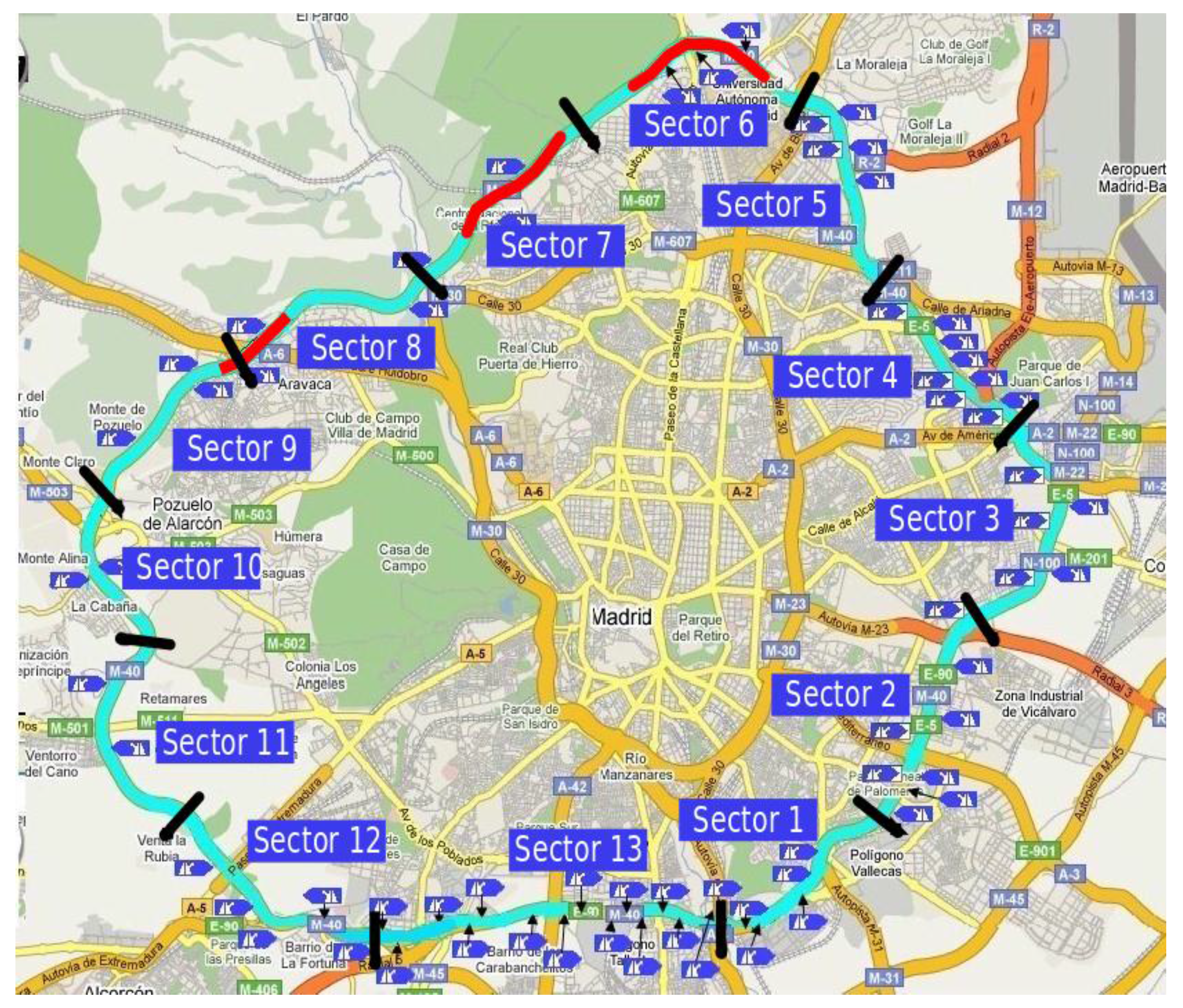
In order to obtain a more extensive trial, the same test was performed over the M40 (an interurban highway with a length of 63 km, (Figure 8) located in Madrid. This highway has 2 carriageways with 3 lanes in each direction. This road counts with a high traffic density and also with some tunnels along the way, which is reflected at the obtained results.

The results of the test are divided in sectors. This decision was taken as there are different zones of the road with tunnels (zones marked in red) that prevent the positioning of the GNSS from being correct. These sections are comprised between exits A-6 and A-1 of the highway. For this reason,

Table 2. Precision test with lane positioning enabled for the mapping system (with computer vision).

Sector	Points Correct	Points Incorrect	Percent
1	1739	261	86.9%
2	1820	180	91.0%
3	1790	210	89.5%
4	1802	198	90.1%
5	1893	107	94.6%
6	1326	674	66.3%
7	1420	580	71.0%
8	1745	255	87.2%
9	1798	202	89.9%
10	1879	121	93.9%
11	1815	185	90.7%
12	1911	89	95.5%
13	2192	326	87.0%

includes two intervals where precision is considerably low, as it is directly related with the position loss of the GNSS. In this table, other results are acceptable according to what was expected from the system.

3.2. CACC System Test

Once corroborated the system precision with the use of computer vision, some specific trials in a real environment in mixed traffic were made with three vehicles equipped with DSRC-INSIA communication modules and the CACC system. These vehicles should also interact during assays with vehicles without communication that are external to the tests. In the following depicted tests, the correct performance of the system is probed in two critical cases of the CACC.

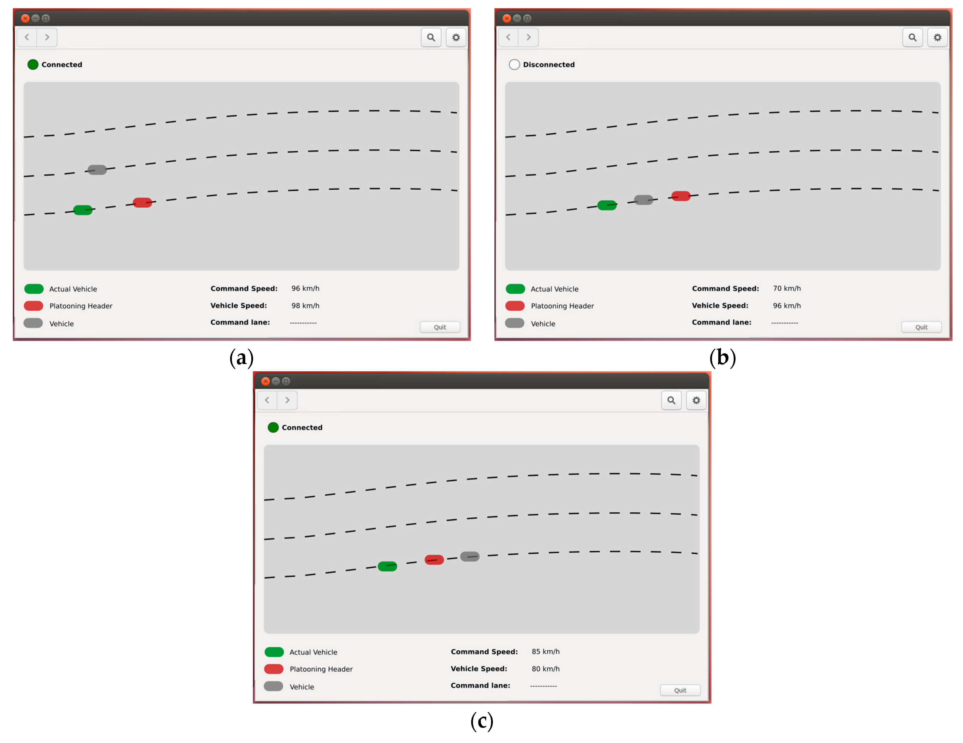
The first critical situation is the insertion of a vehicle between the CACC-equipped members of a platoon driving in the road (cut-in situation). When the new vehicle is set between two vehicles of the platoon, they are forced to restructure the connections. Figure 9 shows the complete process of the maneuver, from the moment of the incident up to the point of stabilization. Firstly, the system formed a platoon of two vehicles (Figure 9a). In the next instant, a new vehicle equipped with a communications module is set between both vehicles of the platooning in the same lane (Figure 9b). In that moment the system detects it and redoes the structure, so the new vehicle serves as the new leader of the last vehicle. Figure 9c depicts the moment when the system is stabilized once again and the platoon moves normally. The vehicle speed decreases from 96 km/h to 86 km/h, because the vehicle has to obtain a safety gap with the new platooning header.

Table 3. Results of the cut-in maneuver tests.

Elapsed Time	Event	Delay (T0 + Tn)
T0	The vehicle is going to change the lane	0 s
T1	The maneuver starts	0.742 s
T2	The systems detects the car	4.260 s
T3	The platoon is disabled	4.272 s
T4	The maneuver has been completed	7.032 s
T5	The platoon is reorganized	7.301 s
T6	The vehicle recovers the safety distance	8.458 s

shows the events considered during the maneuver depicted in Figure 10. The third column marks the time spent by each maneuver into being completed since the instant T₀. The vehicle that makes the lane change maneuver takes 7 s from the start of the movement up to the placement in the new lane. In the data obtained, the system takes 4.260 s to detect the maneuver and 0.012 more to disable the platoon. At instant T₂, the vehicle making the maneuver is placed between both lanes and the system still counts with enough time to lower its speed and set a great enough distance for the maneuver to be completed. The lane change maneuver ends in 7.032 s and in the following 0.279 s the platoon is reestablished. The system takes 1.157 s to stabilize.

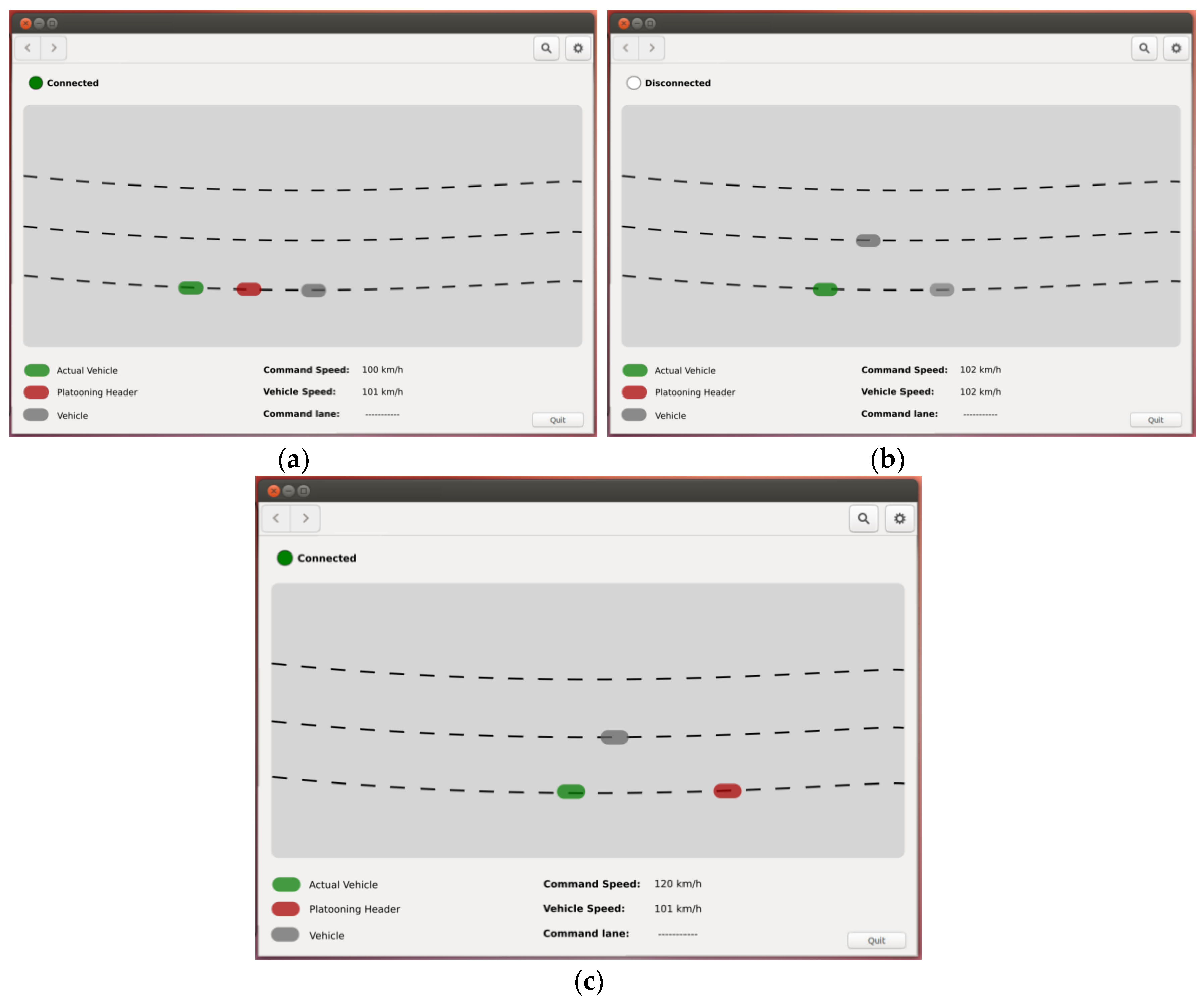
The second trial is made with three vehicles moving on a platoon and the first or second changes the lane on a cut-out maneuver. In the series of screenshots shown in Figure 10 the behavior of the system is appreciated. Figure 8a shows the platoon of three vehicles. Then, the second vehicle changes the lane and the system detects this in order to stop sending instructions to the vehicle’s control (Figure 10b). In that instant, the system looks for the closest vehicle located at the same lane and, if it is feasible, the distance between them is determined. If such vehicle is found, then it is taken as the new leader and the parameters that must be sent to the control are adjusted in order to recover the distance in between (Figure 10c).

Just like the previous situation,

Table 4. Results of the cut-out maneuver tests.

Elapsed Time	Event	Delay (T0 + Tn)
T0	The vehicle is going to change the lane	0 s
T1	The maneuver starts	0.012 s
T2	The systems detects the car coming out	5.105 s
T3	The platoon is disabled	5.160 s
T4	The maneuver has been completed	5.320 s
T5	The platoon is reorganized	6.490 s
T6	The vehicle recovers the safety distance	12.760 s

shows the events to consider from the maneuver made in Figure 10. The vehicle making the lane change maneuver takes 5 s from the start of the movement up to its placement in the new lane. In the data obtained it is appreciated how the system takes 5.105 in detecting the vehicle has gone out of the platoon and 0.055 s more in disabling the latter. Given the nature of the maneuver, it is not necessary for the vehicle to detect which is cutting out of the platoon, as the safety distances are always going to be maintained. Once the platoon is disabled, 1.370 s are needed to locate the closest vehicle in the same lane and set it as the new leader. Due to the space left in the lane by the vehicle that made the maneuver, the system spends 8.270 s in closing the gap. It must be taken into account that the vehicle cannot surpass the maximum speed of the road nor accelerate and decelerate abruptly in order to avoid high fuel consumption.

With these tests, the correct functioning of the system has been validated, as well as its precision and viability. Then, the impact of the introduction of such system on traffic is analyzed using a simulation environment.

4. Simulation Tests

In this second phase, a simulation environment is introduced into the CACC system, which depicts a higher number of vehicles, and the impact over jams and lane cuts in a road, as well as variable traffic density and V2X deployment.

For this matter, Simulation of Urban Mobility (SUMO) [22,23] was chosen as the simulation environment. SUMO is a granularity micro simulator developed by the Institute of Transportation Systems of the German Aerospace Center and is licensed under the General Public License (GPL) version 3.0. SUMO was used as server application and Traffic Control Interface (TraCI) as the Application Programming Interface (API) (and as the Python library) to communicate with the server. Lastly, an outrun header was developed for granting the vehicles with a virtual communications module, which emulates the behavior of the implemented system.

All the vehicles implement the default SUMO modification of Krauß-model for the car-following behavior and the LC2013 model [24] for the lane-change behavior. All the vehicles have V2X communication and the default vehicle’s lane-change model to force a change to the fast lane (in our case the left one) was modified. The fuel consumption model is implemented by SUMO and corresponds to the model gasoline EURO 4 described in Handbook Emission Factors for Road Transport (HBEFA) v3.1 [25]. Furthermore, the purpose of the paper is to show qualitative results but not quantitative ones, so the safety of vehicles is not considered.

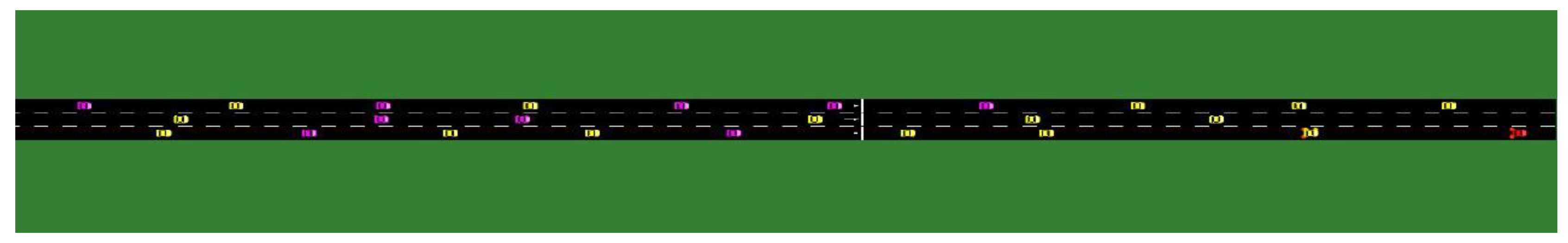
To evaluate the impact of this technology over the traffic flow, two simulations were performed for the case study “Behavior of the CACC system when facing an accident in the highway”. The scenario used in the trials was set in SUMO as a three-lane highway measuring 1 km in length (Figure 11). In such case study, a vehicle stands still at the end of a stretch, blocking the right lane. Simulations register over such stretches the evolution of traffic density with two different flows (low, high) either enabling or not enabling the CACC system in a third of the vehicles.

The CACC system receives the “right lane blocked” message through the communications modules and tries to change the lane as soon as possible. The behavior of the system has been programmed as described in Section 2, meaning that the safety distances are assured for lane changes and adaptation of the vehicle’s speed.

The presented simulations show the behavior of the system when facing situations of dense traffic due to a blocked lane. Trials made lasted for 60 min and always occur in the same scenario. In order to show the improvement obtained over the CACC system, every trial is done twice, with the system enabled or disabled.

At the beginning of every test, the right lane is blocked at 100 m from the ending of the scenario. Whenever the CACC system is enabled, the vehicles received information of the blocked lane 500 m in advance. In the moment that a vehicle that moves through the right lane receives the warning, it analyzes if it can change its lane under safety conditions. If it is possible, then the command is sent to the vehicle’s control system in order to do so. Therefore, two simulations are carried out with different input data of traffic flows: low (1500 vehicles/hour per lane) and high (3000 vehicles/hour per lane). The simulator adjusts the actual flow of vehicles considering road and traffic conditions at each moment. The second situation is quite near to the maximum traffic flow in the bottle neck, so it is considered that the scenario leads to a congested traffic profile.

Table 5. Results of the simulation test.

Traffic Flow	CACC System	Average Speed (m/s)	Average Consumption (mL/Vehicle)	Vehicles Exiting the Road
Low flow	Disabled	21.5	0.064	4340
	Enabled	33.5	0.043	4443
High flow	Disabled	12.6	0.061	6673
	Enabled	26.8	0.052	8863

shows the results with the comparison between a conventional case and the one with the CACC activated. The most notable difference is produced in the flow of exiting vehicles of the road stretch and the average speed. Then, it is possible to reduce the road jam and thus the fuel consumption.

Both flows allow us to see that as the traffic increases, the results obtained when using the CACC system are more evident. In low traffic flow the vehicles exiting the road are almost the same (only 2.3% more vehicles with CACC), but when the system is enabled, the traffic density is lower so the speed is higher with a lower average consumption per vehicle.

In high traffic flow with the CACC system enabled, the average speed is higher (more than twice the average speed with the system disabled) and there are more vehicles exiting the road (24% more vehicles with CACC). In addition, a lower average consumption per vehicle and traffic density are achieved.

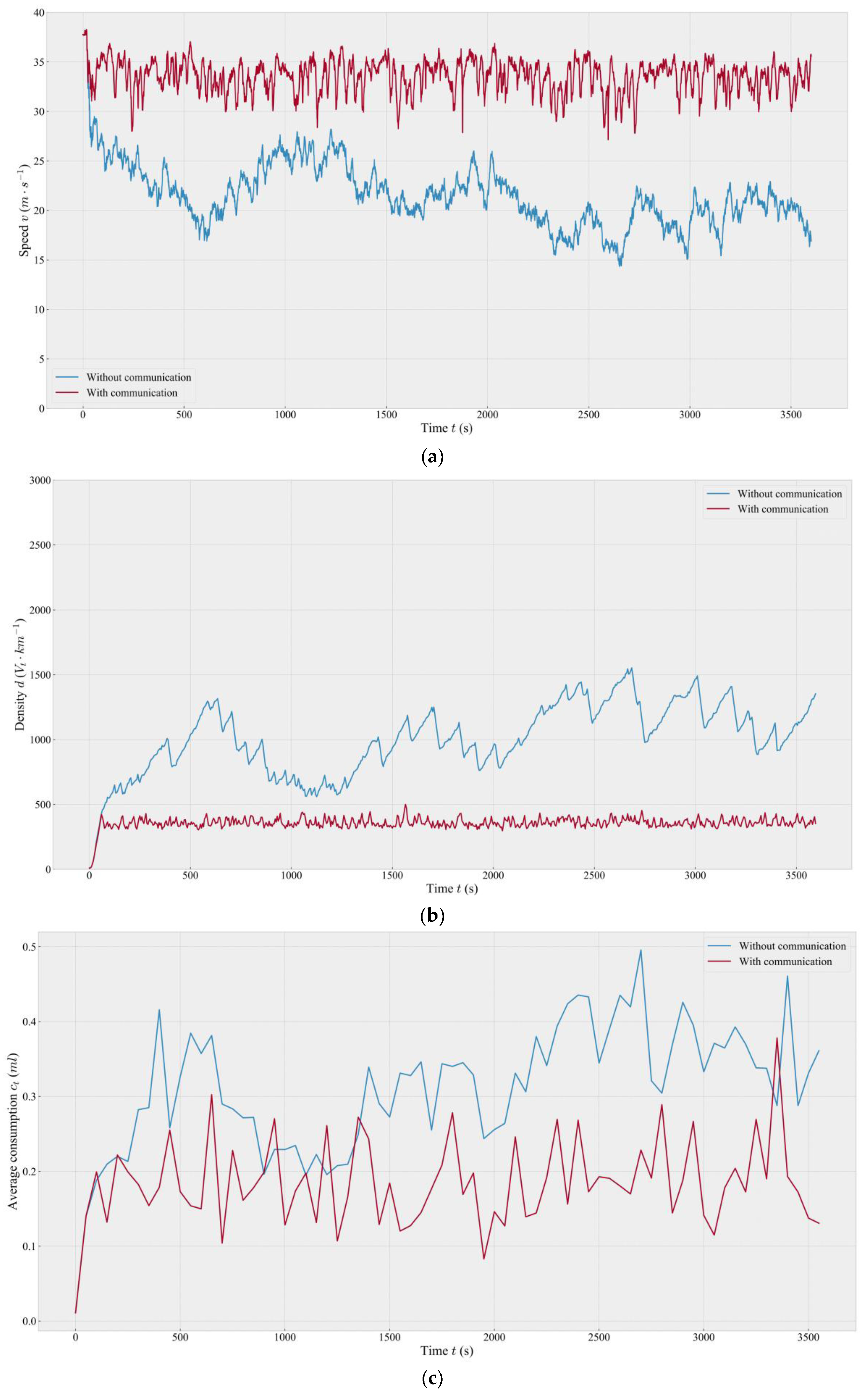
In the Figure 12 and Figure 13, the graphics with the results during the simulation are shown and include:

• Average Speed: average speed of all the vehicles that move along the road.
• Density: number of vehicles in the road stretch.
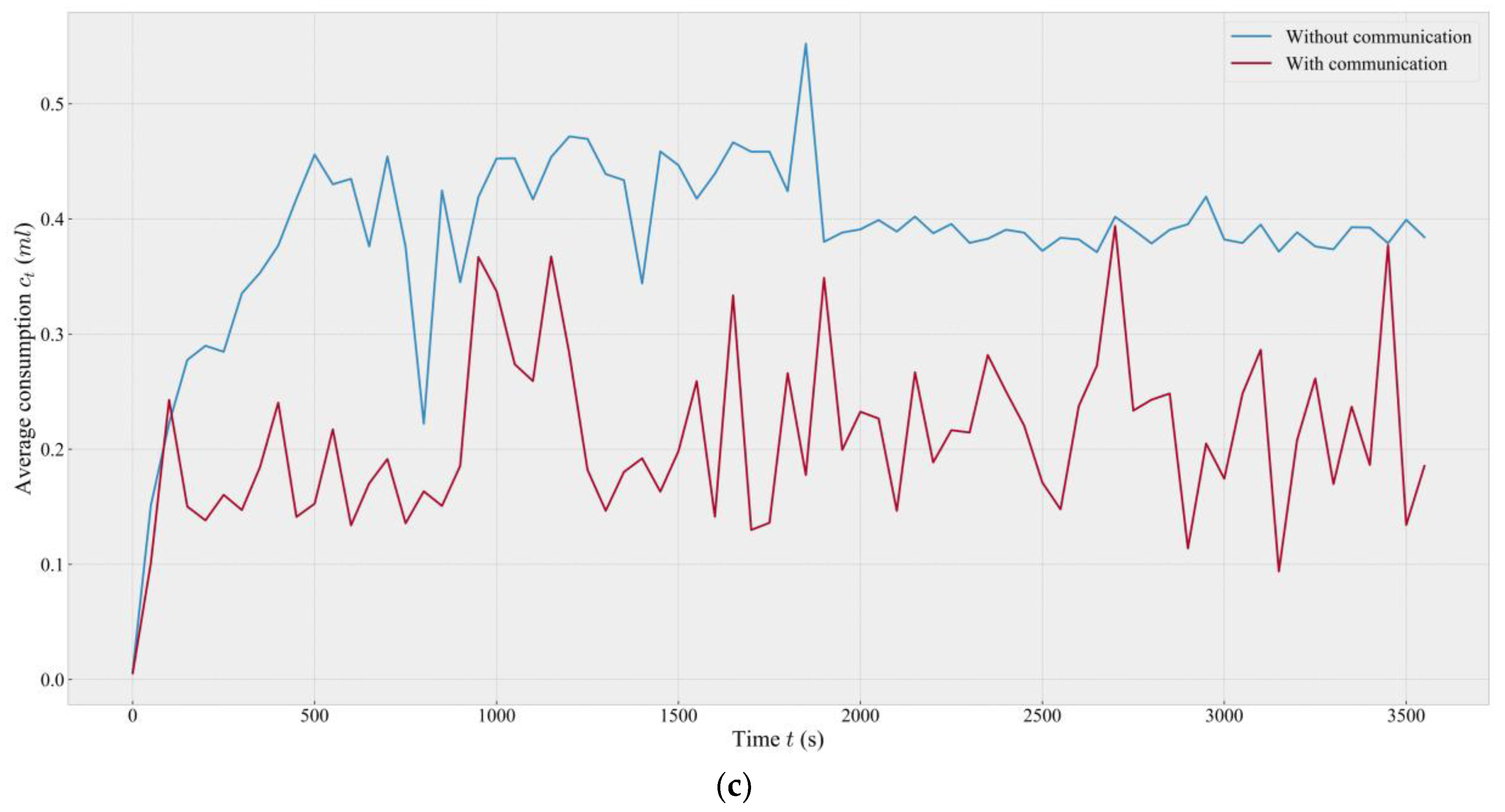
• Average Consumption: average consumption referred to the total number of exiting vehicles.

Figure 12 shows the results of the first trial with input data flow of 1500 vehicles per hour per lane. With the communications and the CACC system enabled it is possible to increase the average traffic speed. By obtaining a higher and constant speed, traffic density is reduced and stabilized to around 400 vehicles. However, without the CACC system, the traffic density tends to increase due to a shock wave that reduces the average speed. This simulation culminates in demonstrating that by using the system, fuel consumption is reduced while traffic is improved.

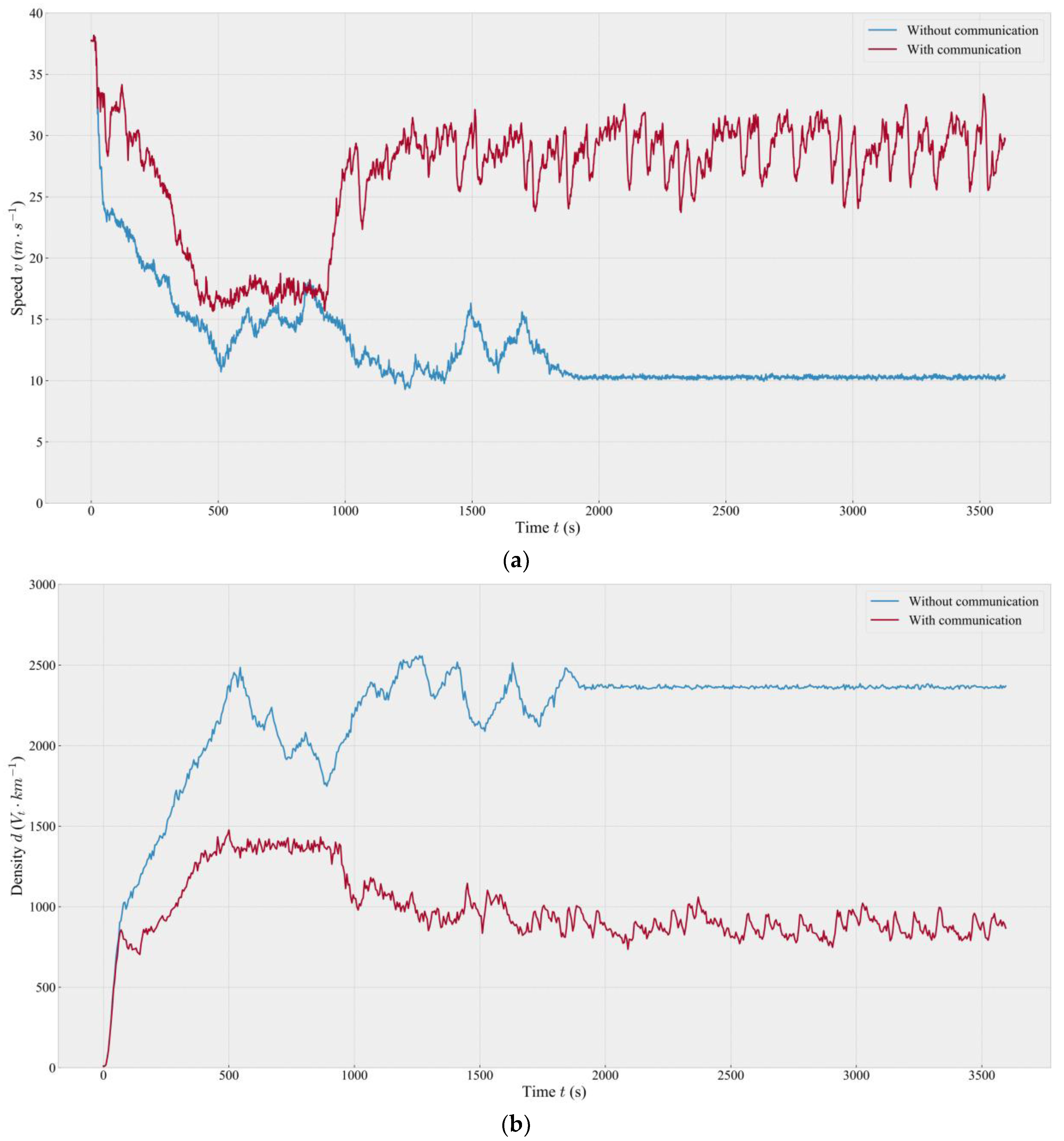
On the other hand, in the simulation of Figure 13, the vehicle flow is duplicated to analyze a situation of congested traffic. The objective of incrementing traffic intensity is to determine the saturation point of the system. With this amount of vehicles, the system with communications and CACC enabled in the first 1000 s of the test is not able to stabilize traffic. After this first stage of the trial, the system stabilized the traffic flow. For this case, the differences between using or not using the system are clearer, with a greater reduction in fuel consumption.

5. Conclusions

In this paper, a CACC system that combines precise positioning at the lane level and V2X communications has been successfully developed. The communications are oriented to the integration of cooperative autonomous driving and the tests in real environments allow for assessment of effectiveness and versatility in different situations.

The proposed mapping combines two technologies, GNSS positioning and computer vision. Through the use of computer vision, the errors obtained in the GNSS positions derived from driving have been corrected. That is, the driver at the time of mapping introduces an error because the vehicle does not remain continuously in the center of the lane, but the proposed algorithm corrects those deviations in the data finally stored in the digital map. It has also been shown that the system solves queries made with a minimum delay (~15 ms).

Despite the fact that the proposed CACC model does not maintain any real-time record of vehicle consumption, nor does it take into account the immediate consumption of the vehicle in its decisions, the system is capable of reducing CO₂ emissions in dense traffic conditions. That is, as demonstrated in the simulations, the actions taken by the system improve the flow of traffic, which results in lower fuel consumption.

V2X communications allow the incorporation of warnings and information from the infrastructure, as shown by way of example in the simulations with a blocked lane. This type of messages reduces congestion and speeds up traffic by reducing fuel consumption and polluting emissions. As has been demonstrated in the tests, the CACC system improves the response because it is able to warn the drivers in advance of situations that the vehicle cannot yet detect (~500 m) with the existing sensors.