A Time for Introducing the Principle of Least Potential Energy in High School Physics

Abstract

Comprehending physical phenomena in topics such as advanced mechanics, quantum mechanics, relativity theory, or particle physics demands one considering the system’s energy, usually under equilibrium constrains. The least potential energy principle (LPEP), which demonstrates an interesting fascinating generalization in physics, is a powerful tool to understand such physics phenomena. Unfortunately, students at high school and universities are exposed to solely considering the forces acting on the system’s particle and apply the Newton’s laws on the system’s particles. Thus, they gain only partial understanding of the physical phenomena they are confronted with and find enormous difficulties to apply energy consideration when needed. If we wish providing students with necessary background to deal with advanced physics, the LPEP should be introduced already in high schools. The current essay provides examples of physics situations in equilibrium where students can apply the LPEP.

1. Introduction

“When I was in high school, my physics teacher—whose name was Mr. Bader—called me down one day after physics class and said, “you look bored; I want to tell you something interesting. “Then he told me something which I found absolutely fascinating, and have, since then, always found fascinating…the principle of least action” [1].

Analyzing physics problems often requires one to understand how to apply conditions for static equilibrium in those problems. Usually, in school physics courses as well as in introductory physics courses students mainly learn that there are two conditions which one has to apply in such problems: (a) zero resultant force; and (b) zero resultant torque about any axis. Equipped with these two conditions a student usually applies them to deal with most physics situations in those courses. However, dealing with more advanced topics such as advanced mechanics, quantum mechanics, relativity theory, or particle physics demands one considering the system’s energy, usually under equilibrium constrains rather than taking into account the forces acting on the system’s particles and calculate their torque. Students who are not used to consider the particle’s energies have difficulties in understanding and analyzing those situations when they are needed. We therefore suggest exposing students to getting used to consider energies involved in physics situations already in high-school and introductory courses at colleges and universities.

In addition, students’ traditional experiences with the concept of energy leads many to view energy as traveling through machines and wires and changing appearances at different points—what Duit calls a quasi-material conception [2]. We believe that this view is caused because students are usually applying the concept of energy in dynamic situations. Consider energies under equilibrium situations and applying the least potential energy principle may assist students to get better understanding of the energy concept as an abstract idea rather than a traveling material.

Herein we first introduce the principle of least potential energy and second, offer three examples taking from hydrostatic, electricity and mechanics to demonstrate how to apply the least of potential energy principle. All the examples are elementary problems which students are expected to be able to easily apply the Newtonian approach to solve them. Knowing one approach will enable them to concentrate on the idea behind LPEP approach.

2. Description of the Principle of Least Potential Energy

The least potential energy principle states that a physical system subjected to conservative forces (i.e., gravitational force), forces that are given by a gradient of conservative field will have the lowest potential energy at a stable equilibrium. In other words, according to this principle and under those conditions a system of bodies at rest will adopt a configuration that minimizes total potential energy. This means that in equilibrium the gradient of the total system’s potential energy equals to zero. Mathematically, we may write this as:

$$\frac{\partial U}{\partial x}=\frac{\partial U}{\partial y}=\frac{\partial U}{\partial z}=0$$

(1)

where U(x, y, z) is the potential energy, which its derivatives are continuous. Equation (1) can be obtained from the zero-resultant force condition in equilibrium ${\displaystyle \sum }\overrightarrow{F}=0$. It is known that when conservative forces are involved we may write:

$$F=-gradU$$

(2)

Since the total force F in equilibrium equals zero we get Equation (1). The principle of least potential energy is actually a private case or a static version of the more general least action principle. According to the least action principle the motion of a physical system from time t₁ to time t₂ is such that the following line integral:

$$S={\displaystyle \underset{t_1}{\overset{t_2}{\int }}(T-U)dt}$$

(3)

where T is the kinetic energy, is an extremum relative to all other paths. It was shown that the path with the minimal action is the one satisfying Newton’s second law [3]. It is clear that for stationary system the principle of least action is reduced to the principle of least potential energy since T = 0 and the potential energy under equilibrium conditions U is time independent. The least action principle, which is one of the greatest generalizations in all physical science, was first formulated by Maupertuis in 1746 [4]. This metaphysical idea was further mathematically developed by the works of Euler, Lagrange, Jacobi and finally formulated by Hamilton and known as Hamilton’s principle [5,6,7].

3. The Use of the Least Potential Energy Principle

3.1. Example a: Fluid Static in a Piston of Small Cross-Sectional Area

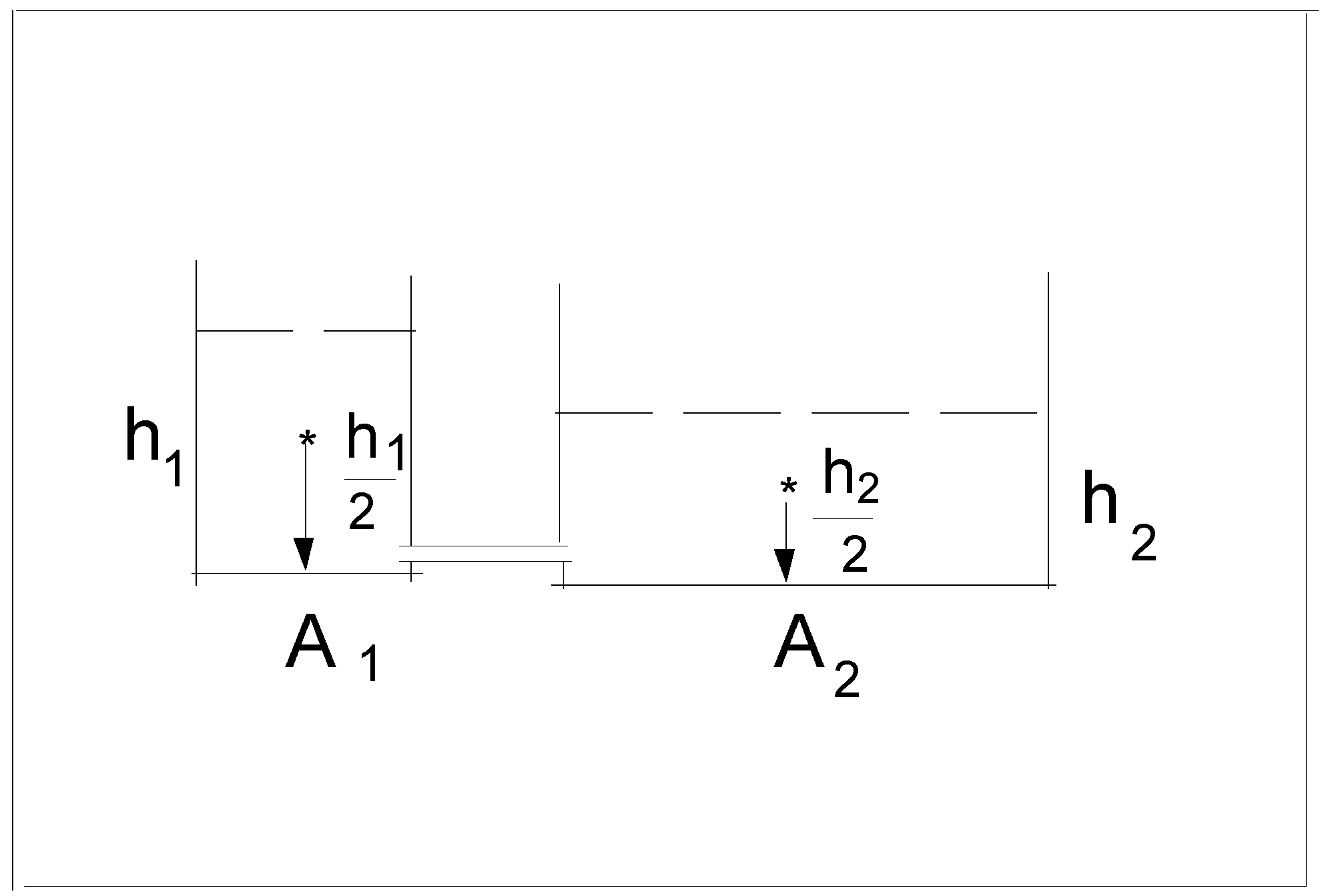
We pour V₀ volume of water into a piston of small cross-sectional area. The bigger pipe area is A1 and the smaller pipe area is A2. The problem is to find the heights h₁ and h₂ of the water in each pipe (see Figure 1) in the equilibrium state.

3.1.1. Newton’s Laws-Based Solution

It is well known [6] that for incompressible fluids the pressure inside the fluid is given by:

$$p=p_0+\rho gh$$

(4)

where $p_0$ is the atmospheric pressure on the surface of the liquid and $\rho$ is the fluid density which assumed to be constant. At equilibrium, the pressures at the bottom of the two pipes are equal thus:

$$p_0+\rho g{h}_1=p_0+\rho g{h}_2$$

(5)

Equation (4) finally yields h₁ = h₂.

3.1.2. Least Potential Energy Principle-Based Solution

Assume that the height of the water in the first pipe of the pistol is h₁ and h₂ in the second. Since the fluid volume in both pipes is V₀ we easily may arrive at the following relation between h₁ and h₂:

$$h_2=(V_0-h_1{A}_1)/A_2$$

(6)

Therefore, the system’s potential energy, taking the density of water as 1, may be expressed in the following formula:

$$E(h_1,h_2)=h_1{A}_1\frac{h_1}{2}g+h_2{A}_2\frac{h_2}{2}g=\frac{g}{2}(h_1^2{A}_1+h_2^2{A}_2)$$

(7)

Inserting the above expression for h₂ into Equation (6) gives the total energy as a function of one variable h₁:

$$E(h_1)=\frac{g}{2}\left(h_1^2{A}_1+\frac{{(V_0-h_1{A}_1)}^2}{A_2}\right)$$

(8)

To find to the stationary points we equate the derivative of Equation (8) and find h₁ which will yield zero. Using elementary calculus, we remain with the following Equation:

$$h_1\left(1+\frac{A_1}{A_2}\right)=\frac{V_0}{A_2}$$

(9)

From Equation (10) we get the following mathematical expression for h₁:

$$h_1=V_0/(A_1+A_2)$$

(10)

This point is indeed a minimum as Equation (11) describes a parabola. From the known relationship between h₁ and h₂ we get:

$$h_2=V_0/(A_1+A_2)$$

(11)

which leads to the final solution that h₁ = h₂.

3.1.3. Discussion Example

Obviously, it is much easier to solve this problem by applying the Newtonian approach. However, it is our belief that from the pedagogical point of view teachers should introduce both approaches of the solution. The Newtonian approach broadens students understanding of the relationship between force and pressure. It also provides them an opportunity to practice Newton’s laws and use them in the context of hydrostatics (and only in mechanical systems). On the other hand, the PLPE approach broaden students perspective on a general idea, a system in equilibrium will be arranged in a way that its potential energy will be the least. Only in introducing both approaches one may gain a deep insight of such a situation. After all, it is not the solution that we are chasing after but rather achieving a deep understanding of the physical situation we confront with [8,9].

3.2. Example b: A System of Point Charges

Four positive electric charges q₁, q₂, q₃ and q₄ are located at the vertexes of a square. What will be the magnitude and position (x, y) of a fifth positive electric charge q₅ so that the point charge system will be in equilibrium (see Figure 2).

3.2.1. Solution Based on Newton’s Laws

If the point charge system is in equilibrium the resultant force on each one of the point charges is zero. If we write this condition on q₅ we get:

$${\overrightarrow{F}}_{1-5}+{\overrightarrow{F}}_{2-5}+{\overrightarrow{F}}_{3-5}+{\overrightarrow{F}}_{4-5}=0$$

(12)

Writing the explicit equations in the system yields the following two equations:

$$\begin{array}{l}{F}_{1-5}\cos {\theta }_1-F_{2-5}\cos {\theta }_2-F_{3-5}\cos {\theta }_3+F_{4-5}\cos {\theta }_4=0\\ -F_{1-5}\sin {\theta }_1-F_{2-5}\sin {\theta }_2+F_{3-5}\sin {\theta }_3+F_{4-5}\sin {\theta }_4=0\end{array}$$

(13)

It is easy to express the sine and cosine of each angel in terms of x and y e.g.,

$$\cos {\theta }_4=x/\sqrt{x^2+y^2}$$

(14)

Inserting those angel expressions as well as Coulomb’s law in Equation (14) we get the following equations:

$$\begin{array}{l}k\left(\frac{q_1{q}_{5}x}{{\left(x^2+{(a-y)}^2\right)}^{3/2}}-\frac{q_2{q}_5(a-x)}{{\left({(a-x)}^2+{(a-y)}^2\right)}^{3/2}}-\frac{q_3{q}_5(a-x)}{{\left({(a-x)}^2+y^2\right)}^{3/2}}+\frac{q_4{q}_{5}x}{{\left(x^2+y^2\right)}^{3/2}}\right)=0\\ k\left(-\frac{q_1{q}_{5}y}{{\left(x^2+{(a-y)}^2\right)}^{3/2}}-\frac{q_2{q}_5(a-y)}{{\left({(a-x)}^2+{(a-y)}^2\right)}^{3/2}}+\frac{q_3{q}_5(a-y)}{{\left({(a-x)}^2+y^2\right)}^{3/2}}+\frac{q_4{q}_{5}y}{{\left(x^2+y^2\right)}^{3/2}}\right)=0\end{array}$$

(15)

where k is the electrostatic constant. Equations (15) are complicate to solve analytically, but can be solved numerically by using appropriate mathematical packages. We skip here the exact solutions of these Equations and present the energy approach for solving this problem.

3.2.2. Solution Based on the Least Potential Energy Principle

First, we write the electrostatic energy function of the system:

$$U(x,y)=U_0+k\left(\frac{q_1{q}_5}{\sqrt{x^2+y^2}}+\frac{q_2{q}_5}{\sqrt{{(a-x)}^2+y^2}}+\frac{q_3{q}_5}{\sqrt{x^2+{(a-y)}^2}}+\frac{q_4{q}_5}{\sqrt{{(a-x)}^2+{(a-y)}^2}}\right)$$

(16)

where U₀ is a the electrostatic energy of the fixed four charges which is constant and does not depend on x and y. Second, we find the minimum of U(x, y) which is now a function of two variables. This is not an easy analytical task at all. However, by using a computer software such as Mthematica this task is doable even in high schools. Moreover, using the computer reduces the technical complexity of solving the problem and enable students to focus on the qualitative understanding of the phenomena. In addition, using Mathematica (or other similar problems) we may also get a contour plot of

$$U(x,y)-U_0$$

(17)

which is a visual display of the potential energy in x-y plane [8,9]. This plot enables finding visually the point of minimum potential energy. Figure 3 shows contour maps for two cases, one where all the charges are identical and equal to 1c and the second where q₁ = 1.1 (for simplicity we choose a = 1 m and k = 1). It can be seen that the point of minimum should be in the middle of the green area (x, y) = (0.5, 0.5) (the green color represents the area of minimum potential energy) for the symmetric case and slightly to the right to the middle for the asymmetric case (x, y) = (0.523, 0.477). Also, it can be seen in the contour map that near the point charges the potential energy is the highest (the red color represents the area of high potential energy) [10,11].

3.2.3. Discussion Example b

By using the Newtonian approach students may deepen their understanding of the electrical forces, they can practice the technique to calculate components of the forces in the x and y axes, and practice applying the resultant zero constrain. However, again, it is our belief that from the pedagogical point of view teachers should introduce also the LPEP approach. The students might see that in a stable equilibrium the system’s particle will be arrange in such as to lowest the system’s potential energy [8,9,10].

Also, using the computer and plotting the two-dimensional maps of the potential energy might provide the students an opportunity to use more than verbal and mathematical representation of knowledge. It is known in the literature that using different representations of the same phenomena might deepen the understanding of the phenomena that the student is confronting with. Moreover, the contour plot of the energy provides global information about the electrostatic energy distribution of the point charge system and does not focus on the desired answer of the problem. The student does not only understand where the point of the lowest potential energy is but also may comprehend why it is not possible to put the fifth point charge near to one of the other four point charges. This means that those plots may provide the students an opportunity to further discuss the problem rather than be satisfied from the answer of where this point should be. One may argue that using computer software is out of the scope of school curriculum. We on the other hand believe that with the advantage of technology and the availability of computers in school teachers might find that such an experience might interest students [9,10,11].

3.3. Example c: Body Connected to a Spring on an Incline

In this example the students are asked to find the displacement x of a block mass m, connected to spring (with stiffness constant k) and being in rest on a frictionless incline. The incline forms an angle α with the horizontal (see Figure 4).

3.3.1. Solution Based on Newton’s Laws

The free diagram is shown in Figure 4. We choose the origin of the coordinate system at the point where the spring is upstretched. Then we write Newton first law for the x and the y axes:

$$\begin{array}{l}mg\sin \alpha -kx=0\\ N-mg\cos \alpha =0\end{array}$$

(18)

From the first Equation we get that:

$$x=mg\sin \alpha /k$$

(19)

3.3.2. Discussion Example c and Solution Based on the Least Potential Energy Principle

The total potential energy of the block consists from two parts on is gravitational potential energy and the second is elastic potential energy. Using the same coordinate system, the total potential energy of the block is given by:

$$U(x)=\frac{1}{2}k{x}^2-mgx\sin \alpha$$

(20)

which is a graph of a parabola. Note, that the gravitational potential energy is negative since it is below the reference level. Deviating Equation (21) with respect to x yields:

$$U^{\prime }(x)=kx-mg\sin \alpha$$

(21)

Equation (21) to zero and solve for x we obtain that x_min = mgsinα/k and that the equilibrium is stable.

Discussion. The Newtonian approach gives the solution for the problem even if we include static friction between the block and the incline. For this case it is easy to show that:

$$x=\frac{mg(\sin \alpha -\mu \cos \alpha )}{k}$$

(22)

where μ is the coefficient of static friction. Since we defined the LPEP for equilibrium states where only conservative forces are acting, we cannot treat in this framework dissipative forces such as the friction force [10,11,12,13]. Thus, it seems that for system subjected to nonconservative forces the Newtonian approach is advantageous. It is interesting that for this example we can use an extended potential energy $\tilde{U}$ which gives the correct answer:

$$\tilde{U}=\frac{1}{2}k{x}^2-xmg\sin \alpha -x\mu mg\cos \alpha$$

(23)

where the last term in Equation (23) is the work done by the friction force μmgcosα, but for writing this we had to go back to free-body diagram.

3.4. Example d: Loaded Flywheel

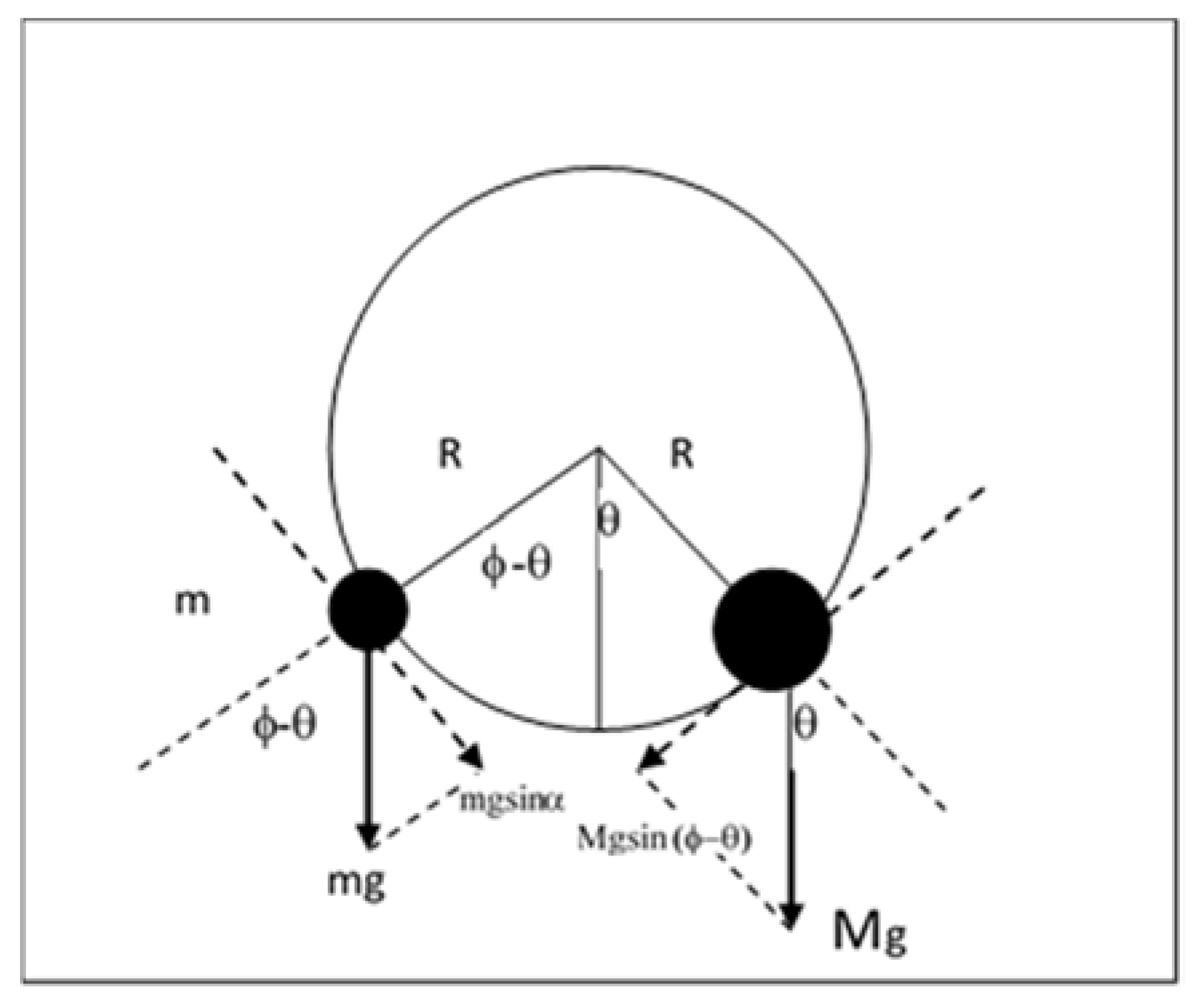
The following problem, taken from Lemones [7], demonstrates how one can distinguish between stable and unstable equilibrium states by using the LPEP approach [7]. Two-pointed masses M and m are fixed on the rim of massless flywheel of radius R hanging on its center. The angular separation between the two masses is ϕ (see Figure 5). The tangential component of the weight of each mass corresponds for a torque, which try to rotate the wheel around its center. Use the circular polar coordinate θ to find the position of equilibrium.

3.4.1. Solution Based on Newton’s Laws

In this problem we use the torque condition for static equilibrium. The two torques acting on the wheel’s center are ${\tau }_1=Rmg\sin \theta$, and ${\tau }_2=Mg\sin \left(\varphi -\theta \right)$. Applying the zero-resultant torque condition we obtain,

$$RMg\sin \theta -Rmg\sin (\phi -\theta )=0$$

(24)

Using the following trigonometric formula:

$$\sin (\phi -\theta )=\sin \phi \cos \theta -\cos \phi \sin \theta$$

(25)

and after simple algebraic manipulations we get the following solutions,

$$\begin{array}{l}{\theta }_1=arc\cot \left(\frac{M}{m\sin }+\cot \phi \right)\\ {\theta }_2={\theta }_1+\pi \end{array}$$

(26)

The solution indicates that there are two equilibrium points. To find the stable equilibrium state there is a need to check whether small displacements from the equilibrium points will result in a restoring torque tending to return the particle to the equilibrium position or whether it will tend to push it further away. There is no formalism that can directly be used to examine this point. Thus it might not be an easy task for novices.

3.4.2. Solution Based on the Least Potential Energy Principle

The potential energy of the system can be written as (the reference level is the bottom of the wheel):

$$U(\theta )=mgR(1-\cos (\phi -\theta ))+MgR(1-\cos \theta )$$

(27)

and the first derivative with respect to θ is:

$$U^{\prime }(\theta )=gR(m\sin (\phi -\theta )-M\sin \theta )$$

(28)

Solving $U^{\prime }\left(\theta \right)=0$ we the same solutions θ₁ and θ₂. In order to test the stability of the solutions we have to check the sign of $U^{″}({\theta }_1)$ and $U^{″}({\theta }_2)$. Instead of doing this we prefer to show the graph of the potential energy for real numerical values m = 0.5 kg, M = 1 kg, R = 0.5 m, ϕ = 2π/3 and g = 9.8 m/s².

Figure 6 shows that ${\theta }_1$ is indeed a stable equilibrium while ${\theta }_2$ is unstable equilibrium as it maxima of the potential energy.

3.4.3. Discussion Example d

When the system has more than one equilibrium point it is much easier to find which one is stable using the LPLE method, where the physical problem reduced to a regular mathematical problem of finding extremum points of a function which can be even done graphically [14,15].

4. Conclusions

The purpose of this essay was to advocate the use of LPEP in equilibrium situations already on first steps of physics courses. Usually, exposing students to energy consideration at school relates to dynamic situations. Typical question is to find the speed of a ball sliding on a frictionless loop-the-loop track at different points. Students, however, do not learn to consider energies in equilibrium situations. In the current essay we suggested to introduce to students the following two aspects while dealing with equilibrium: (A) The forces acting on the system’s particles, meaning applying the Newtonian rules (zero resultant force and zero resultant torque); and (B) the potential energy of the particles in the systems. Our examples show that such treatment has the following advantages: (1) Deep understanding of equilibrium situations—the two aspects are complementary and each contributes to the comprehension of the equilibrium phenomena. Exposing student to only one aspect the student may get only part of the picture; (2) Variety of presentations—the Newtonian approach is more algebraic in nature and students are thus exposed to mathematic Equations. Potential energy, on the other hand, which is a scalar, may be also described by graphs. For instance, the potential energy in the point charges problem was presented by contour map. Often the most effective way to describe, explore and summarize a set of numbers—even a very large set—is to look at a visual display of those numbers. A good representation of data, both graphically and numerically, may enable powerful and sufficient inferences, obviating the use of delicate and subtle statistical constructs [16]. Indeed, the point charge problem could be solved visually by looking at the contour graph and identifying the area of the lowest potential energy (the greenest color in the graph). In addition, from the graph a student can relate to other questions that he was not directly asked for. For instance, that the potential is a symmetric and that the region of highest potential energy is near the four-point charges; (3) Overcoming misconceptions—considering energy only in dynamic situations as being usually done in the traditional physics class may explain some misconceptions described in the literature such as described by Gilbert and Pope [17]: (I) energy is obvious activity; (II) energy is a dormant ingredient within objects, released by a trigger; (III) energy is seen as type of fluid transferred in certain processes. We believe that since in equilibrium there is nothing being “transferred” the students might better understand the idea of energy as an abstract concept which one can use to deal with physical phenomena. In addition, one of the rigorous misconceptions is relating to force as being energy. Equilibrium situations such those that were presented herein presented two solutions one is the Newtonian approach; the other is the energy approach in parallel. This might contribute to the students to grasp the relationship between force and energy.

Stability characterization of the system. The LPEP gives us information about the stability of the system by further classifying the extremum points as minimum, maximum or inflections points. Local minima are stable equilibria, local maxima and inflections points are unstable equilibria while finite regions of constant potential are regions of neutral equilibrium. In the long term we observe only stable and neutral equilibria as the unstable ones are sensitive to small perturbations that drive the system towards stable equilibria.

It is our hope that choosing three simple examples, known to most teachers as a framework for explaining how to use the LPEP in equilibrium as well as the rational provided here will convince teachers to introduce it before their students.

This paper provided four examples of how the Least Potential Energy Principle (LPEP) can be applied. The author suggests that the LPEP should be introduced in high schools, as its application could provide students with the deeper understanding of physical phenomena, as well as provide ground for their dealing with advanced physics afterwards. The examples are the following: ‘Fluid static in a piston of small cross-sectional area’, ‘A system of point charges’, ‘Body connected to a spring on an incline’ and ‘Loaded Flywheel’, where for each of them solutions based on both Newton’s laws and LPEP are provided. All are classic physics problems that students deal with in high school. This paper’s contribution is twofold. At first, it contributes to the discussion of restructuring energy education, and, secondly, provides an example of how to better prepare the next generation of scientists, which is especially required in fields like theoretical Physics and Mathematics that are selected by only few in tertiary education.

Although this subject doesn’t learn in most places, understanding of the least potential energy can leads to improve the other field of physics. By understanding very basic unique phrases and simple calculation the student can exposed to new physics that they didn’t learn before. In order to leads this subject to be universal, this program should have developed into new fields that some of them written these days. Houle et al. [18] and Hrepic et al. [19] claim that the right way teaching at the high school can avoid losing student at the colleges and the university. This way has to be universality with known pedagogical methods that encourage student to understand the subject. Voice, as an example, teachers avoid to teach it at the high school level since the complexity of mathematics formula. These students when they come to colleges and university, exposed to the complexity of the mathematics formula, some of them leave, some continue with a real understanding but the major part may understand the math, but not the voice subject as part of waves. So, if you teach the student at the high school the qualities aspects when they are young (at least at the beginning), the student come to the universities with the right tools that can govern on the mathematical level with real understanding. This pedagogical aspect has to suitable for all the student all over the world. Of course, each program has the right synonym. Also, here, the least potential energy should have learned in universality way and with different level. Means, at the high school the level should be with lower math level with a lot of phrases and explain in much more basic way. Furthermore, the Universal Design for Learning Principle roles have to assimilate in the least potential energy in the global learning. First, as I mention the level of high school student and universities are different, so, high school student doesn’t have to finish all the program. Second, the teachers have to learn a glossary of key terms at the beginning of the course, unit, or week. This glossary includes links to online resources where students can find definitions of key terms (e.g., subject encyclopedia through the library). Furthermore, all the lecture should be recorded, so the student from the different level could learned from that. After this recorded class, the student can learn from hard copy note book with different level of exercises. The program should to provide short videos that emphasize or highlight relationships between course concepts, especially when introducing new ideas. Of course, all of that should be in different languages.

References

- Feynman, R.P.; Leighton, R.B.; Sands, M. The Feynman Lectures on Physics; Addison-Wesley: Boston, MA, USA, 1964; Chapter 19. [Google Scholar]
- Duit, R. Should energy be illustrated as something quasi-material? Eur. J. Sci. Educ. 1987, 9, 139–145. [Google Scholar] [CrossRef]
- Hanc, J.; Tuleja, S.; Hancova, M. Derives Newton’s laws of motion from the Principle of Least action. Am. J. Phys. 2003, 71, 386–391. [Google Scholar] [CrossRef]
- Glass, B.; Temkin, O.; Straus, V. Forerunners of Darwin; Johns Hopkins University Press: Baltimore, MD, USA, 1959. [Google Scholar]
- Hilderbrandt, S.; Tromba, A. The Persimmons Universe; Springer: New York, NY, USA, 1996. [Google Scholar]
- Meriam, J.L.; Kraige, L.G. Engineering Mechanics, Statics; John Wiley & Sons: Hoboken, NJ, USA, 2002; p. 287. [Google Scholar]
- Lemons, D.S. Perfect Form; Princeton University Press: Princeton, NJ, USA, 1997. [Google Scholar]
- Courant, R.; Robbins, H. What Is Mathematics? Oxford University Press: Oxford, UK, 1951. [Google Scholar]
- Wolfram, S. The Mathematica Book, 3rd ed.; Wolfram Media/Cambridge University Press: Kwun Tong, UK, 1996. [Google Scholar]
- Denzler, J.; Hinz, A.M. Catenaria Vera—The true catenary. Expo. Math. 1999, 17, 117–142. [Google Scholar]
- Taylor, E.F. A call for action. Am. J. Phys. 2003, 71, 423–425. [Google Scholar] [CrossRef]
- Belmonte, A.; Shelley, M.J.; Eldakar, S.T.; Wiggins, C.H. Dynamic patterns and self-knotting of a driven hanging chain. Phys. Rev. Lett. 2001, 87, 114301. [Google Scholar] [CrossRef] [PubMed]
- Mareno, A.; English, L. The stability of the catenary shapes for a hanging cable of unspecified length. Eur. J. Phys. 2008, 30, 97. [Google Scholar] [CrossRef]
- Fallis, M.C. Hanging shapes of nonuniform cables. Am. J. Phys. 1997, 65, 117–122. [Google Scholar] [CrossRef]
- De Sapio, V.; Khatib, O.; Delp, S. Least action principles and their application to constrained and task-level problems in robotics and biomechanics. Multibody Syst. Dyn. 2008, 19, 303–322. [Google Scholar] [CrossRef]
- Eshach, H.; Schwartz, J.L. Understanding Children’s Comprehension of Visual Displays of Complex Information. J. Sci. Educ. Technol. 2002, 11, 333–346. [Google Scholar] [CrossRef]
- Gilbert, J.; Pope, M. Small group discussions about conception in science: A case study. Res. Sci. Technol. Educ. 1986, 4, 61–76. [Google Scholar] [CrossRef]
- Houle, M.E.; Barnett, G.M. Students’ conceptions of sound waves resulting from the enactment of a new technology-enhanced inquiry-based curriculum on urban bird communication. J. Sci. Educ. Technol. 2008, 17, 242–251. [Google Scholar] [CrossRef]
- Hrepic, Z.; Zollman, D.A.; Rebello, N.S. Identifying students’ mental models of sound propagation: The role of conceptual blending in understanding conceptual change. Phys. Rev. Phys. Educ. Res. 2010, 6, 020114. [Google Scholar] [CrossRef]
Figure 1.
Schematic illustration of the fluid static in a piston of small cross-sectional area problem.
Figure 2.
Four positive electric charges are fixed in the corner of a square. We have to find the place where a fifth positive charge will be in equilibrium. The repulsive forces acting on the charge are illustrated schematically in the diagram.
Figure 3.
Contour plots showing the energy function U(x, y) − U0 for k = 1 and a = 1 m. The symmetric case where all the charges are identical is shown at left and the asymmetric case where q1 = 1.1c, c is shown at the right.
Figure 4.
A block mass m which is connected to a spring with stiffness k, rests on a frictionless incline which makes an angle α with the horizontal. The forces acting on the block are the normal force N, the weight mg and the force exerted by the spring −kx.
Figure 5.
Loaded massless flywheel with two fixed point masses M and m.
Figure 6.
Potential energy (in Joules) of the loaded wheel vs. the polar coordinate θ. θ1 = 0.5236 is the stable equilibrium while is unstable equilibrium. Numerical values used: m = 0.5 kg, M = 1 kg, R = 0.5 m, ϕ = 2π/3 and g = 9.8 m/s2.
© 2018 by the author. Licensee MDPI, Basel, Switzerland. This article is an open access article distributed under the terms and conditions of the Creative Commons Attribution (CC BY) license (http://creativecommons.org/licenses/by/4.0/).
Share and Cite
MDPI and ACS Style
Ben-Abu, Y. A Time for Introducing the Principle of Least Potential Energy in High School Physics. Energies 2018, 11, 98. https://doi.org/10.3390/en11010098
AMA Style
Ben-Abu Y. A Time for Introducing the Principle of Least Potential Energy in High School Physics. Energies. 2018; 11(1):98. https://doi.org/10.3390/en11010098
Chicago/Turabian StyleBen-Abu, Yuval. 2018. "A Time for Introducing the Principle of Least Potential Energy in High School Physics" Energies 11, no. 1: 98. https://doi.org/10.3390/en11010098
Note that from the first issue of 2016, this journal uses article numbers instead of page numbers. See further details here.