Large-Signal Stability Modeling for the Grid-Connected VSC Based on the Lyapunov Method


Department of Energy Technology, Aalborg University, 9220 Aalborg, Denmark
*
Author to whom correspondence should be addressed.
Energies 2018, 11(10), 2533; https://doi.org/10.3390/en11102533
Submission received: 24 August 2018
/
Revised: 14 September 2018
/
Accepted: 19 September 2018
/
Published: 22 September 2018
(This article belongs to the Section F: Electrical Engineering)
Abstract
:In this paper, a Lyapunov-based method is used in order to determine the stability boundaries of the grid-connected voltage source converter (VSC). To do so, a state space model of the VSC is used to form the Lyapunov function of the system. Then, by using the eigenvalues of the Lyapunov function, the system stability boundaries will be determined. It is shown that the grid-connected VSC works in its stable mode when all of its Lyapunov function’s eigenvalues are positive. The proposed model validity is tested by time-domain simulation. Simulation results show that the method is credible in determining the stability margin of the grid-connected VSC.
1. Introduction
As the penetration of Distributed Generations (DGs) increases, the stability assessment of the power systems becomes more complicated. This is because of the very detailed control systems of the power electronic-based (PE-based) units [1]. Although the stability of the conventional power systems is a well-explored field of research, the integration of the PE-based units with the main grid and its penetration bring new challenges to the transmission and distribution system operators in respect of the reliability and the stability, which leads to new perspectives of the grid codes [2]. What makes the stability assessment of the PE-based energy sources different from the conventional power generators is in their control systems and their inertia. Generally, a PE-based unit has a small inertia compared with a conventional power plant. On the other hand, in the modeling of DGs connected to the power systems, typically called grid-connected Voltage Source Converters (VSCs), the control system plays a vital role [3]. In this manner, stability assessment of the control systems of the PE-based units is the matter of importance, which is well studied in [4,5,6,7,8,9], and still is a matter of concern for researchers [10,11].
There are many methods in the stability assessment of the power systems, such as Nyquist stability analysis, eigenvalue-based methods, root locus analysis, etc. [4,5,6,7]. Generally, methods developed for the stability analysis can be divided into two main categories: time-domain analysis, and frequency-domain analysis methods [4]. In time-domain analysis, the non-linearity behavior of the system is taken into account, while in most frequency-based methods linear techniques are applied in order to assess the stability [12]. The main disadvantage of the time-domain-based methods is that it is time consuming; hence, its computational burden increases as the system size becomes large. Therefore, these methods are not practical for large-scale systems [13].
On the other hand, regarding frequency-based methods, linear techniques are applied in order to analyze the system behavior. These linear techniques may apply into linear or linearized systems. PE-based power systems are nonlinear-based in their nature. In order to use linear-based stability analysis methods for PE-based power systems, linearization techniques should be applied. In addition, these methods are only credible around one equilibrium operating point of the system [14]. With this in mind, both linear and nonlinear methods have their merits and demerits. This is mentioned in Table 1.
To overcome these drawbacks, nonlinear-based methods are developed in order to evaluate the stability of the power systems [8,15]. One of the main sub-categories of the nonlinear stability assessment of the power systems belongs to the energy function-based (EF-based) methods (also known as Lyapunov-based methods). The idea behind the EF-based methods is that the system is called stable if and only if its energy is positive and the derivative of its energy with respect to the time is not positive [29]. Based on that, many attempts have been done in order to assess the stability of the PE-based power systems, which is reviewed in [8]. Although, Lyapunov-based methods may show either the system works in its stable mode or not, it will not be useful in designing the control parameters. On the other hand, as its nonlinear nature, Lyapunov-based methods are credible for all operating points of the system. Therefore, it is appropriate to use it for large-signal stability assessment [30]. As a nonlinear stability assessment technique, the Lyapunov stability method is credible for both small signal and large-signal stability analysis. The main challenge in determining the stability boundaries using the Lyapunov stability method is to determine the energy function. Although some attempts have been done in order to determine the energy function of a system, there is no straight method in order to define it [15,29]. In most cases, PE-based units are considered as energy sources that are coupled into the main systems [9,31]. In order to find the energy function for the PE-based units, the synchronous machine equivalent of the VSC is defined in [32]. Although synchronous machine equivalent of the VSC shows appropriate results both in simulation and experimental tests, the converter may not act as its synchronous machine equivalent in all conditions, which leads to some drawbacks of the equivalent synchronous machine of the VSC [33,34]. The stability analysis of the equivalent synchronous machine of the VSC can be assess by its linear approximation model [34]. On the other hand, an energy function is well developed for the synchronous machines, which can be used for the VSC as well. Yet, the main question of defining the step by step method for determining the energy function is not been answered [5,22,32,34].
By applying Lyapunov-based methods, it is possible to control the PE-based unit independent of the system parameters in addition to handling large-signal disturbances [35]. In [36], the Lyapunov-based stability analysis is applied on a reduced-order model of the system in order to assess the large-signal stability of the system. Results are compared with the full-order eigenvalue-based stability analysis, and it is shown that the energy function can appropriately determine the stability boundaries of the system. In [22], a current controller is designed based on the Lyapunov function in order to control the active and the reactive power of the converter. in this paper, the error of the control parameters of the system from their reference values is considered as the key components of the energy function. Although the format of the energy function and how to assess the stability of the system based on the Lyapunov function is described in this paper, the relation between the energy function and the system state variables are not cleared. In [23], state variables of the system are considered in the energy function. Although the stability boundaries are determined using the direct Lyapunov method, the energy function parameters’ effect on the system stability is not explained in the paper. The idea of using the Lyapunov function for the large-signal stability analysis is widely accepted, as it is still an interest of researchers [37]. Although, the Lyapunov function is used in order to assess the stability of the PE-based units in the literature, there is less attention in systematic analyzing the stability of the PE-based systems using the EF. To the best knowledge of the authors, there is less attention on determining the energy function of the system systematically. However, the impact of the energy function parameters on finding the stability boundaries is not yet investigated.
In this paper, a systematic analyzing method of the grid-connected VSCs is developed based on the Lyapunov function of the system. To do so, current control system and the time delay caused by switching of the converter are modeled in state space form. Then, the matrix energy function is introduced in order to find the boundaries of the stability. A parametric form of the Lyapunov function is presented in a matrix format in order to find the marginal point of the stability. It is shown that as long as the energy function is defined in a credible format, i.e., in positive definite form, the system will stay stable in stability region. Therefore, the stability boundary is independent of the defined energy function. In addition, the eigenvalue-based stability analysis is presented in order to validate the systematic energy function-based method. In this manner, the main contributions of this effort are listed as follows:
- Proposing a systematic way in order to find the Lyapunov function of the grid-connected VSC based on the system state variables.
- Parametric analysis of the energy function for the stability of the grid-connected VSC.
- Studying the effect of the linearization on determining the stability margin of the grid-connected VSC.
Another issue to be mentioned is that controlling in the dq frame leads to coupling between d and q element. Therefore, decoupling terms are needed in order to have an appropriate control system. The time delay is not typically considered in the decoupling process. As the time delay is not considered in decoupling, shown in the simulation results section, the method gives an approximation of the conservative stability boundaries.
The rest of the paper is organized as follows. Section 2 presents the concept of the Lyapunov function and its application in stability of the system. The parametric Lyapunov function and its validity to compare with linear methods, e.g., eigenvalue-based stability assessment, are proposed in Section 3. Simulation results are illustrated in Section 4. Finally, the conclusion of the paper is presented in Section 5.
2. Lyapunov-Based Stability Assessment
In this section, the basic concept of the Lyapunov-based stability assessment is explained. Consider a synchronous generator with voltage value of , connected to the grid with voltage through a line with reactance as shown in Figure 1. The active power transferred from synchronous generator to the grid can be calculated as follows:
Assume that the reactance of the transmission line abruptly changes from to , which is less than . The mechanical power produced by the generator () is considered to be fixed, while the electrical active power produced by the generator will change into due to the new transmission reactance value as shown in Figure 2. The difference between mechanical and electrical active power can be calculated in the swing equation as follows:
where M is the total moment of inertia of the generator. and are synchronous generator rotor angle and its mechanical active power, respectively.
The difference between mechanical and electrical power will cause accelerating in the rotor of the generator. This will continue until the mechanical and electrical power become equal. After that, the electrical active power will continue increasing until it reaches . If there is no damping in the system, electrical active power will continue oscillating between and . By adding a damping factor in the system, the electrical active power may eventually converge to . The area of and show the amount of energy added to the system during the acceleration time and absorb by the system during deceleration period, respectively. Based on Lyapunov stability definition, and should be equal in order to have a stable equilibrium operation point.
For the generator, the energy function may be defined in many forms. Here, the Lyapunov function is considered as follows [38]:
where is the angular velocity of the synchronous generator rotor angle is the stable equilibrium point generator angle. The energy function may be divided into two parts: the kinetic and potential energy, as follows:
The potential energy is zero at stable equilibrium point and it reaches its maximum value when becomes zero. As there is a limitation in system states value, there is maximum value for the potential energy. If the system’s maximum kinetic energy is more than the maximum value of the potential energy, then the system will continue accelerating beyond the maximum value of the potential energy. This leads the system into instability. The value of the energy function is always positive, and its derivative with respect to the time is negative in order to decelerate the system into the stable equilibrium point. This concept is widely used in the stability analysis of the system. In the next section, its use in relation to the grid-connected VSCs will be discussed.
3. Parametric Lyapunov-Based Stability Analysis of the Grid-Connected Voltage Source Converter (VSC)
3.1. Modeling of the Grid-Connected VSC
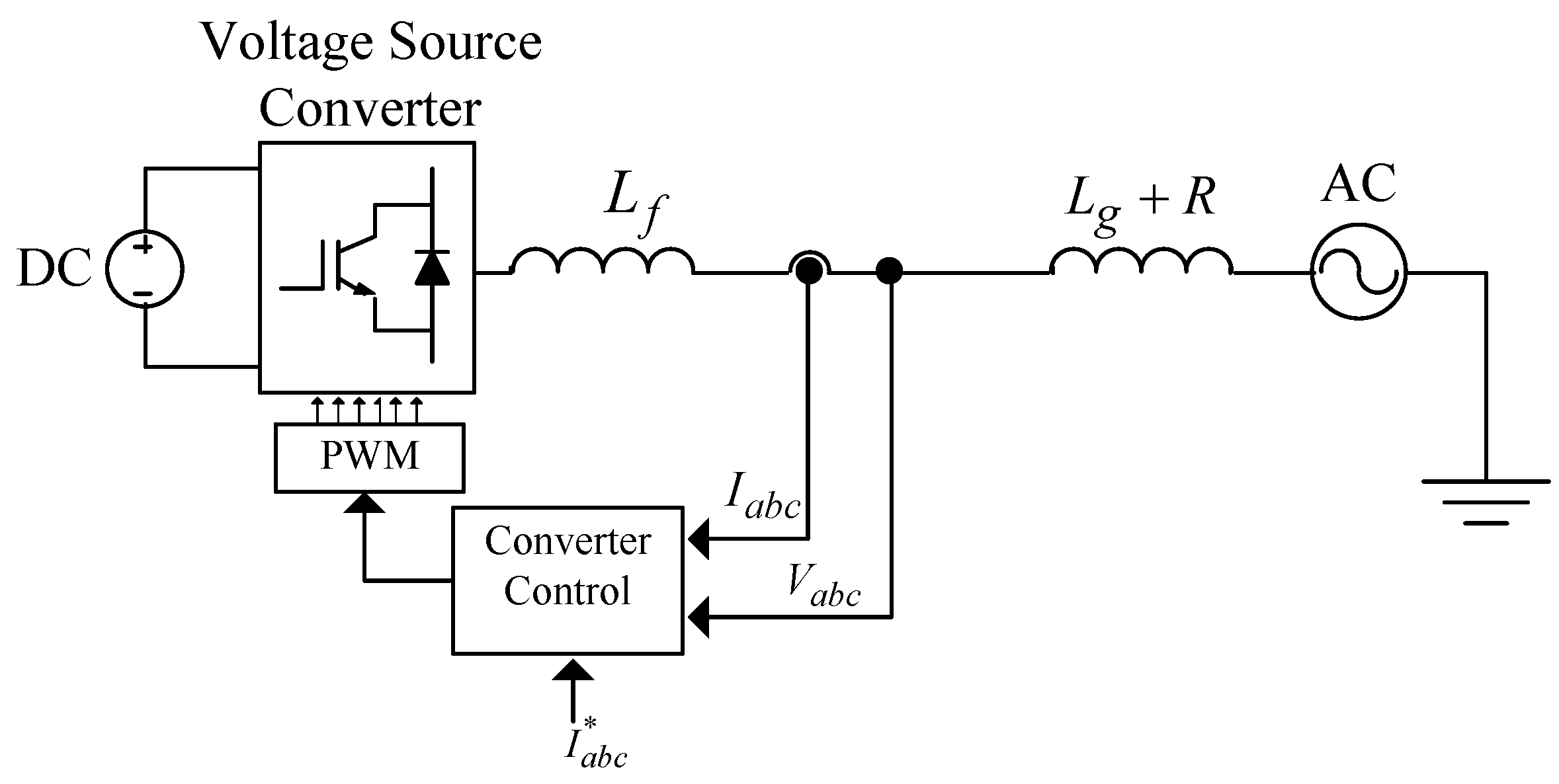
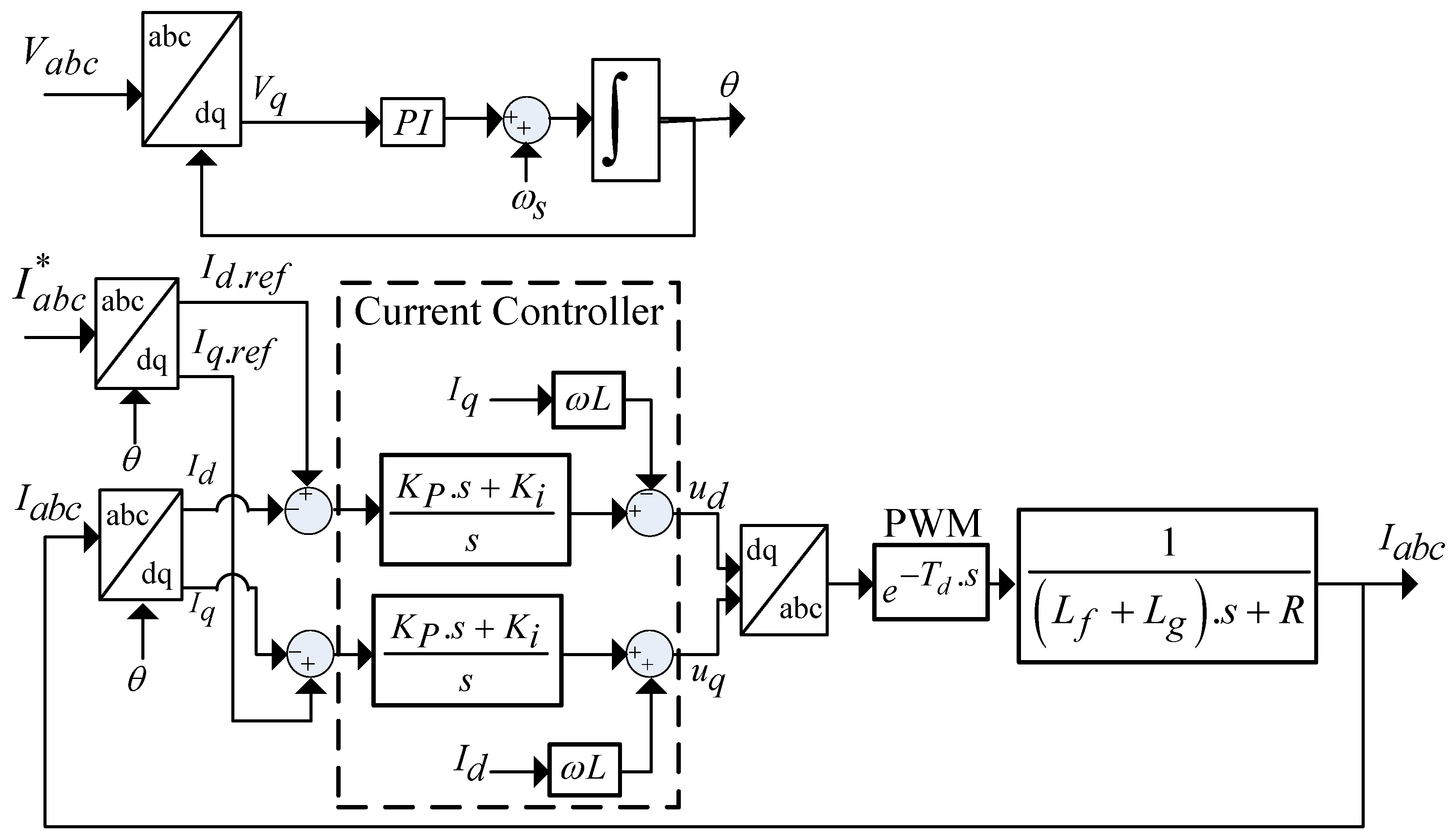
In this section, the Lyapunov function is used in order to determine the stability boundaries of the grid-connected VSCs. To do so, the VSC is considered as it works in the grid-feeding mode. In this manner, only current control and time delay are considered in the control loop and the plant, as shown in Figure 3.
In this model, the converter is connected to an ideal DC voltage source, and the grid is assumed to be an ideal three-phase voltage source. Therefore, and the VSC’s voltage at the Point of Common Coupling (PCC) is assumed to be fixed. The control system is designed in the dq rotating frame, hence Park’s and Clarke’s transformation are applied in Iabc in order to control Id and Iq as related to the current in the d- and q-axis, respectively. The combination of the Clarke and Park transformation is used to transfer Iabc into Id and Iq is presented as follows:
where is the voltage phase, as the voltage at the PCC is fixed by the grid side, which makes it stable in order to use for the Phase Locked Loop (PLL). This can be determined by using the PLL, as shown in Figure 4, where is an approximation of the voltage phase [39].
The current reference can be determined by using desired active and reactive power as follows:
where P and Q are desired active and reactive power of the VSC, respectively. In addition, Vd and Vq are voltage values at the PCC in the d- and q- axis, respectively. As the voltage is assumed to be fixed, Id and Iq can be controlled directly by choosing their related reference values (Id.ref and Iq.ref). The whole process of the current control is shown in Figure 5.
To consider the time delay into the model, the pade approximation is used in order to linearize the nonlinear behavior of the delay.
where Td is time delay, e.g., 1.5 times of the converter’s sampling time period.
Considering a state variable for each integrator of the system , the state space equations of the current control is presented as follows for the d axis:
where matrices A, B, and C are:
where Ki and KP are the integrator and proportional coefficients of the PI current controller, Td is the time delay of the PWM and the discrete implementation, L and R are the inductor and the resistor of the converter filter plus the grid impedance, respectively.
The state space equations for the q-axis is similar to the state space equations in d axis, yet only the d axis control is presented for the sake of brevity. In the Lyapunov-based stability assessment of the system, only the Matrix A of the system is used, which is discussed in the next part.
3.2. Systematic Lyapunov-Based Stability Method
To assess the stability of the system by using the energy function method, first the Lyapunov function and its derivative with respect to the time should be determined. The Lyapunov function may include physical variables or the whole state variables of the system. Here, as the detailed model of the system is presented, the Lyapunov function is defined based on all state variables of the system. In this manner, the Lyapunov function and its derivative with respect to the time are defined as follows:
where x and xT are the state variables vector and its transpose vector, respectively. A is the state matrix of the system, which is defined in the Section 3.1. Here, Q is defined as follows:
P and Q are numerical matrices, which are explained next. If both P and Q are positive definite, then the system works in the stable mode. By defining the P, Q will be determined based on the system state matrix. Alternatively, by defining Q, P can be determined. Here, Q is defined in a specific positive definite manner, then system stability is determined based on the analyzing the matrix P. Before that, the definition of the positive definite matrix is explained.
Assume Q is an nn positive definite matrix. Then, it should satisfy the following inequality:
where s1, s2, …, and sn are non-zero real numbers. Alternatively, if all eigenvalues of the Q have a positive real part, then it is positive definite. In order to calculate the eigenvalues of the system, the following equation should be solved:
where I is an identity matrix. indicates the eigenvalues of the system. Here in this approach, a specific form of Q is defined as (15), then, for every positive real value of a, Q satisfies (13).
In order to proof the mentioned claim, applying (2) into (14) will result in the following:
which is always positive for all positive value of a and non-zero values of , , and , , , and .
With this in mind, next, P will be determined based on the system state matrix, as shown in (9), and the Q. Assume P as follows:
where , …, and are matrix P’s element. For a stable system, P should be a positive symmetric matrix, e.g., Based on the definition of A in (10), and the definition of the Q and P presented in (11) and (16), respectively, six equations with six variables, as shown in (17), should be solved.
By solving the equations in (17), P can be determined. Then, if P is positive definite, then the system is stable. It can be seen from (17) that the values of the P’s element are dependent on the proportional and integral gain of the current controller in addition to the time delay caused by the converter and the system-impedance L. This means that P is dependent on the controller parameters in addition to the grid impedance. The eigenvalues of every positive definite matrix have real parts. By using this fact, the stability of the system will be determined. As long as the eigenvalues of the P have positive real parts, the system is stable.
It is worth mentioning that if P is positive definite, then the Lyapunov function becomes positive for all state vectors and hence the system is stable for all operating points. On the other hand, if P is not positive definite, then the Lyapunov function may have a positive, negative, or zero value. In case that the Lyapunov function is negative, then the system is unstable. With all this in mind, in order to evaluate system stability eigenvalues of the P and the energy function may be monitored. More detailed information is discussed in the results section.
4. Simulation Results
In this section, simulation results of the stability assessment using the Lyapunov function method for the grid-connected VSC is discussed. In this way, a grid-connected VSC as shown in Figure 3, with a controller as shown in Figure 4 and Figure 5 is developed in Matlab/Simulink in order to validate the method developed in Section 3. The system parameters and configurations are illustrated in Table 2.
To evaluate the stability of the system by using the Lyapunov-based method, the first step is to choose an appropriate Q matrix, which should be positive definite. This can be done by using (15). Here, a is considered to be equal to 1, as shown in (19).
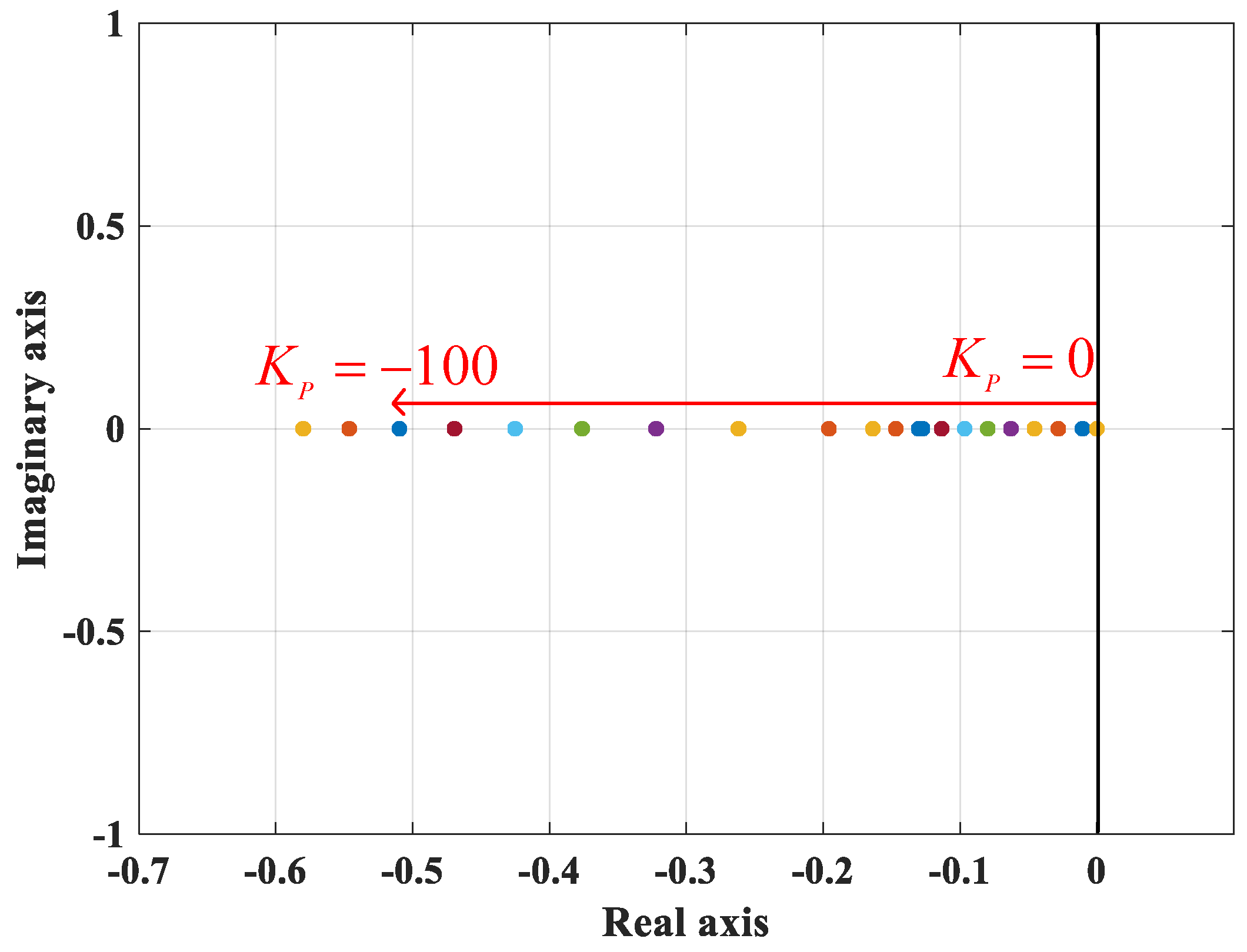
Next, the P will be determined by using (16) and (17). Then, by determining the eigenvalues of P, the stability of the system can be evaluated. Considering system parameters introduced in Table 1, by choosing Ki = 600 and KP increasing from zero to infinity, eigenvalues of P is illustrated in Figure 6. As KP increases from zero to 133, the value of one of the eigenvalues of the P increases. After that, by increasing KP from 134, one of the eigenvalues gets a large negative number. The absolute value of one of the eigenvalues decreases by increasing KP from 134 to infinity, and it gets closer to the imaginary axis. Considering the eigenvalues of P, it can be concluded the value of KP can be increased until 133 in order to work in the stable mode. In addition, if the value of KP is negative, two out of three eigenvalues of P, as shown in Figure 7, become negative.
Considering Figure 6 and Figure 7, it can be concluded that the value of KP should be between 0 and 133 in order to keep the P positive definite, which leads to positive value of the energy function for all state of the system. Moreover, as Q is positive definite, defined in (11), then the derivative of the energy function with respect to the time is negative. This leads to a stable mode of the system. Furthermore, as can be seen in Figure 7, by using negative proportional gain for the current controller, the real part of the P matrix will become negative. This means that as the proportional gain of the current control becomes negative, P matrix is not positive definite anymore, which explicates as the instability of the system.
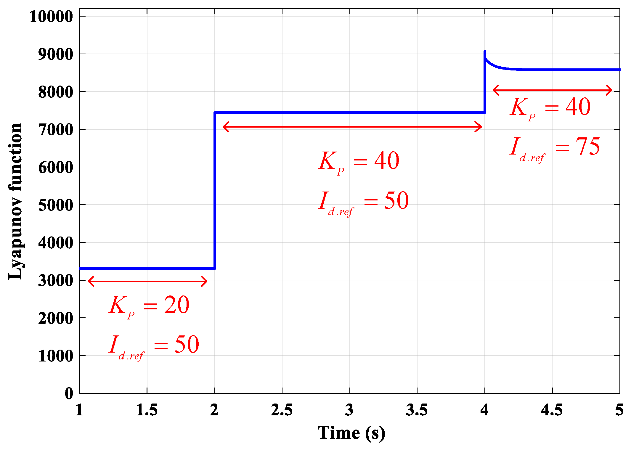
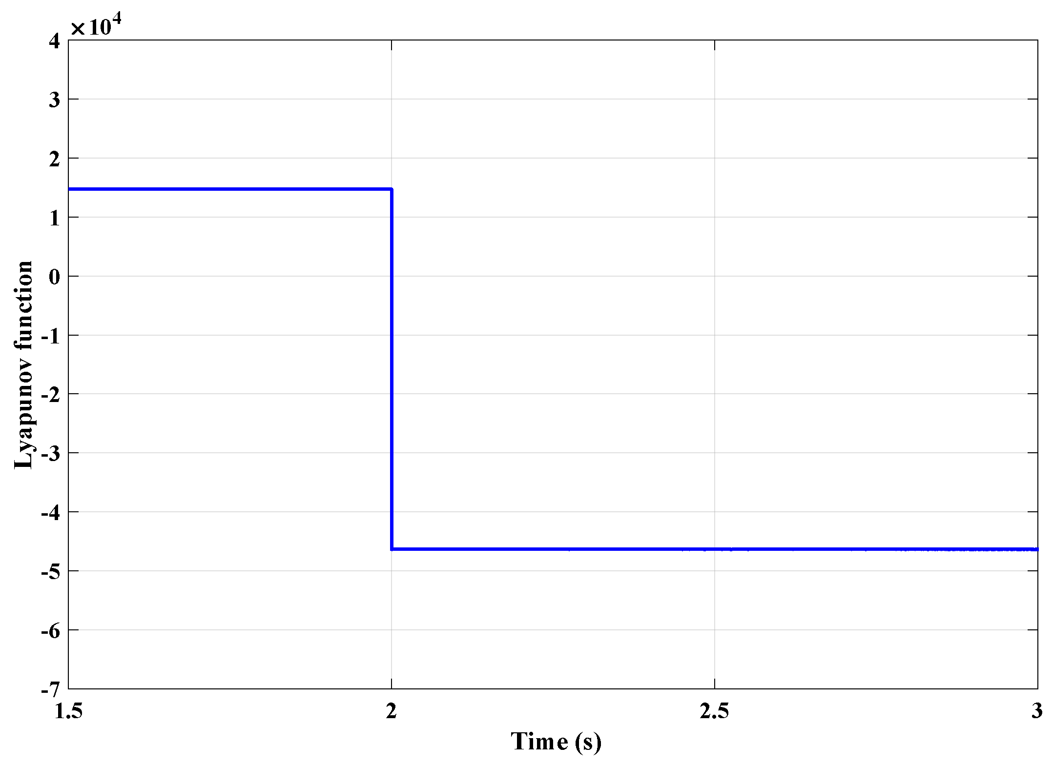
Considering the time-domain simulation of the energy function, simulated by Matlab/Simulink tool, if it is positive and its derivative with respect to the time is negative, it cannot be concluded that the system is stable. The reason is that even if P is not positive definite, the energy function may have a positive value. On the other hand, if the energy function is negative, then the system is unstable. The reason is that if the energy function is negative, then P is not positive definite, and it has at least one eigenvalue with a negative real part. These are shown in Figure 8, Figure 9 and Figure 10. In Figure 8, the system works in its stable mode with KP = 20 and Ki = 600. At t = 2 s, the value of the KP changes into 40. The energy function is still positive. Considering the P’s eigenvalues shown in Figure 6, the system will maintain stable for all state conditions. With a step change in the reference current at t = 4 s, the energy function will stay positive. Meanwhile, the current response to the step change in the reference for the mentioned condition is illustrated in Figure 9. Figure 10 shows the energy function value of the system with Id.ref = 50 A and change in KP from 70 to 140 at t = 2 s. The energy function value becomes negative at t = 2 s, which means that the system works in its unstable mode.
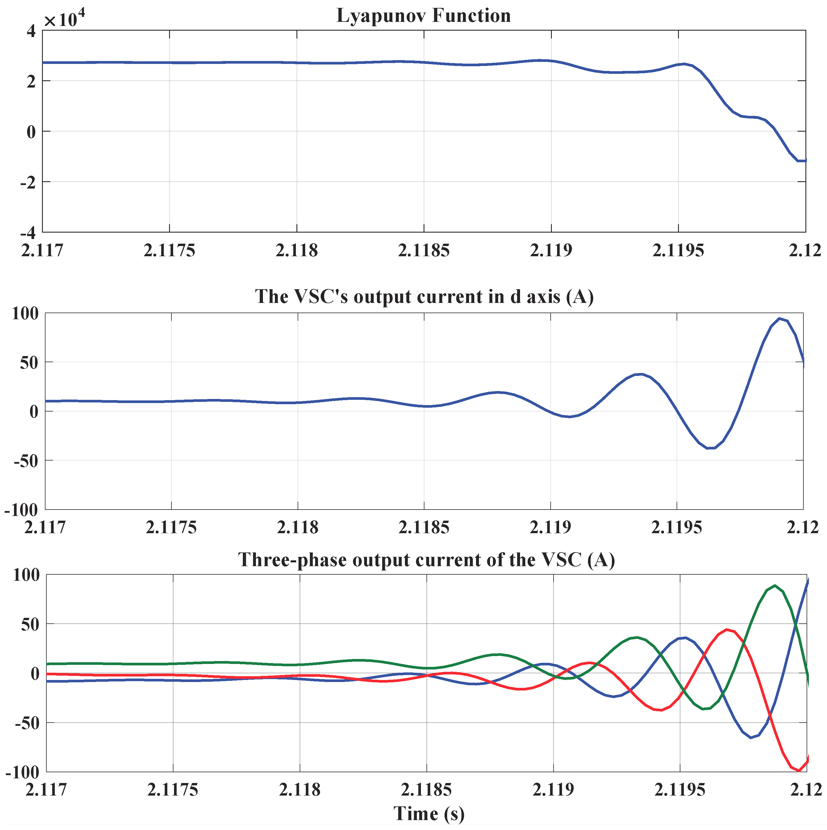
The simulation results of the current control response also show the instability in tracking the reference current after changes the KP from 80 to 160, as shown in Figure 11. The instability will not happen exactly at t = 2 s, which is due to the nonlinear behavior of the system and the time delay caused by the PWM and sampling period. Although the instability in the output current of the VSC, as shown in Figure 11, leads to a negative value for the Lyapunov function at t = 2.1198 s. In order to focus more on the behavior of the Lyapunov function, only the energy function and the output current of the VSC for the period from t = 2.117 s to 2.12 s is shown in Figure 11. This behavior of the system can be predicted by monitoring the eigenvalues of P.
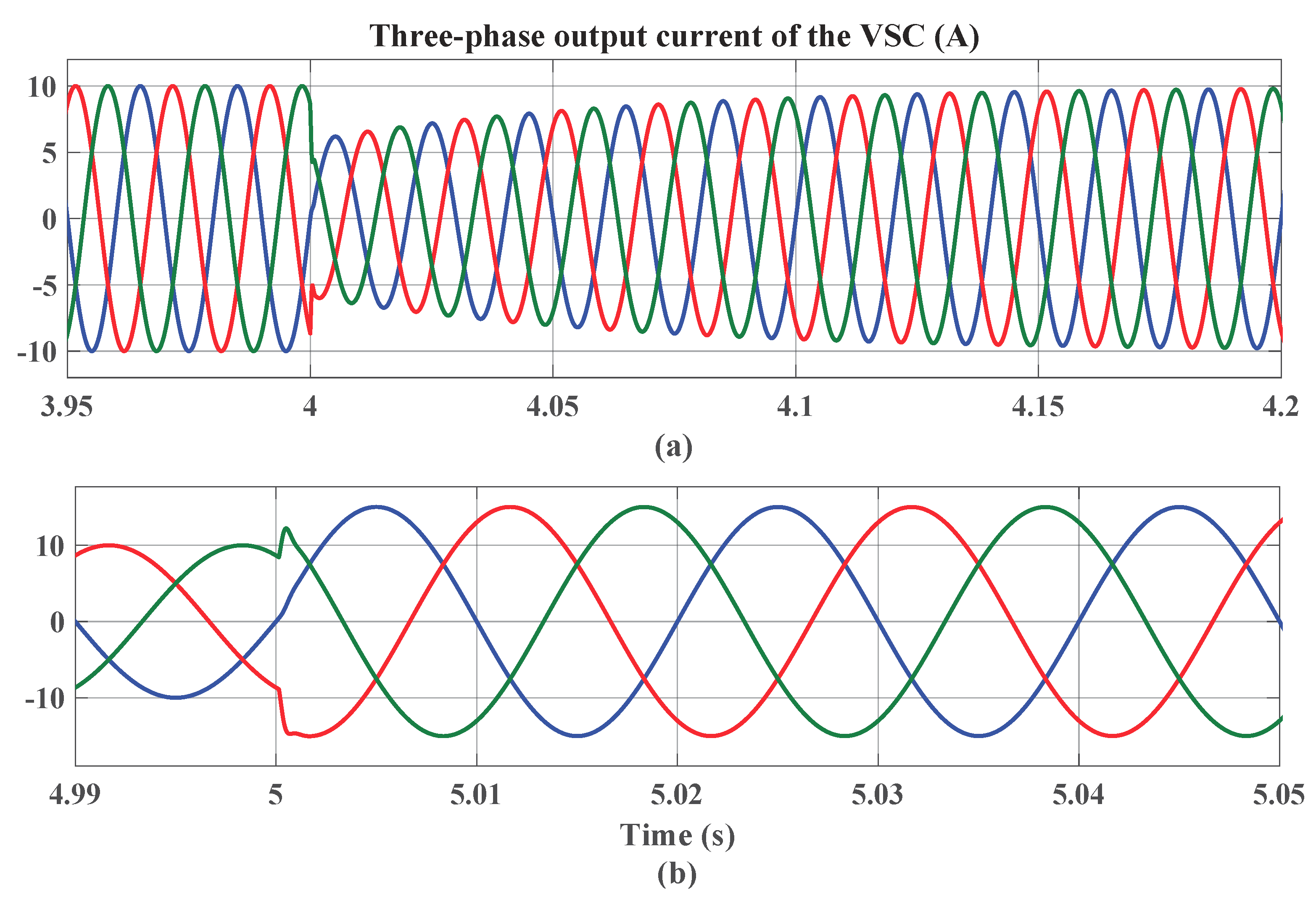
On the other hand, if a fault happens on the grid side, a voltage sag will typically appear. This can be simulated by a step change on the grid-side voltage magnitude. In case that the system works in its stable limits (Kp and Ki are set in their stable limits), the Lyapunov function will be positive, and the output current will follow a step change in the reference current. Although the step change in voltage reference will cause a change in the output current of the VSC, as there is no voltage controller in the control system, the output current will be changed with a large time constant. This is shown in Figure 12. A 50% voltage sag happens at t = 3 s and lasts for 1 s. Moreover, the current reference is changed from 10 A to 15 A at t = 5 s. As it can be seen in Figure 13, a step change in the reference current will be followed by the output current almost immediately, while the output current cannot follow a step change in the voltage output voltage with the same time step.
5. Conclusions
In this paper, a parametric representation of the Lyapunov-based stability assessment is presented in order to determine the stability margin of the grid-connected VSCs. To do so, a current control presented in dq rotating frame including the time delay is considered as the system controller. The matrix Lyapunov function is presented as the identifier of the stability status of the system. It is shown that as long as the Lyapunov function is positive and its derivative with respect to the time is negative, the system is stable. Unless, the system will converge into instability. Therefore, the system stability boundary is independent of the Lyapunov function’s parameters. on the other hand, it is shown that the stability boundary of the grid-connected VSC is dependent on the physical system parameters, such as line impedance, in addition to the control system parameters.
As the systematic approach is proposed in order to evaluate the stability boundaries of the system, therefore, this method is expandable to the evaluation of other control systems. By doing so, the energy function of other control systems can be defined in the parametric form. Then it can be evaluated if the system stability is dependent on the energy function or not. In this paper, it is shown that the stability boundaries are independent of the energy function parameters.
On the other hand, although a systematic approach is developed in order to determine the parametric energy function of the system in order to evaluate the stability of the system, the proposed method suffers from some drawbacks. In the proposed method, only one VSC is considered as the case study. in the real case, there can be some converters connected to the main grid. By expanding the system size, the computation burden will become larger, which means that in order to evaluate the system stability boundaries, more time is consumed. This is not appropriate for the transient stability analysis. A recommendation to deal with this drawback is to use a reduced-order model of the system.
Author Contributions
All authors contributed to prepare the manuscript equally.
Funding
This work was supported by the Aalborg University.
Conflicts of Interest
The authors declare no conflict of interest.
References
- Rocabert, J.; Luna, A.; Blaabjerg, F.; Rodriguez, P. Control of Power Converters in AC Microgrids. IEEE Trans. Power Electron. 2012, 27, 4734–4749. [Google Scholar] [CrossRef]
- Altin, M.; Göksu, Ö.; Teodorescu, R.; Rodriguez, P.; Jensen, B.B.; Helle, L. Overview of recent grid codes for wind power integration. In Proceedings of the 2010 12th International Conference on Optimization of Electrical and Electronic Equipment, Piscataway, NJ, USA, 20–22 May 2010. [Google Scholar] [CrossRef] [Green Version]
- Blaabjerg, F.; Teodorescu, R.; Liserre, M.; Timbus, A.V. Overview of Control and Grid Synchronization for Distributed Power Generation Systems. IEEE Trans. Ind. Electron. 2006, 53, 1398–1409. [Google Scholar] [Green Version]
- Kundur, P.; Balu, N.J.; Lauby, M.G. Power System Stability and Control; McGraw-Hill: New York, NY, USA, 1994; Volume 7. [Google Scholar]
- Ogata, K. Modern Control Engineering; Prentice-Hall: Boston, MA, USA, 2010; Volume 5. [Google Scholar]
- Zarei, S.F.; Mokhtari, H.; Ghasemi, M.A.; Blaabjerg, F. Reinforcing Fault Ride Through Capability of Grid Forming Voltage Source Converters Using an Enhanced Voltage Control Scheme. IEEE Trans. Power Deliv. 2018. [Google Scholar] [CrossRef]
- Bottrell, N.; Prodanovic, M.; Green, T.C. Dynamic Stability of a Microgrid With an Active Load. IEEE Trans. Power Electron. 2013, 28, 5107–5119. [Google Scholar] [Green Version]
- Kabalan, M.; Singh, P.; Niebur, D. Large Signal Lyapunov-Based Stability Studies in Microgrids: A Review. IEEE Trans. Smart Grid 2017, 8, 2287–2295. [Google Scholar]
- Andrade, F.; Kampouropoulos, K.; Romeral Martínez, J.L.; Vasquez Quintero, J.C.; Guerrero, J.M. Study of large-signal stability of an inverter-based generator using a Lyapunov function. In Proceedings of the 40th Annual Conference of the IEEE Industrial Electronics Society, Dallas, TX, USA, 30 October–1 November 2014. [Google Scholar]
- Li, X.; Hua, L. Stability Analysis of Grid-Connected Converters with Different Implementations of Adaptive PR Controllers under Weak Grid Conditions. Energies 2018, 11, 2004. [Google Scholar]
- Harnefors, L.; Finger, R.; Wang, X.; Bai, H.; Blaabjerg, F. VSC Input-Admittance Modeling and Analysis Above the Nyquist Frequency for Passivity-Based Stability Assessment. IEEE Trans. Ind. Electron. 2017, 64, 6362–6370. [Google Scholar] [CrossRef]
- Safaee, A.; Woronowicz, K. Time-Domain Analysis of Voltage-Driven Series–Series Compensated Inductive Power Transfer Topology. IEEE Trans. Power Electron. 2017, 32, 4981–5003. [Google Scholar] [CrossRef]
- Wang, J.; Liang, J.; Gao, F.; Dong, X.; Wang, C.; Zhao, B. A Closed-Loop Time-Domain Analysis Method for Modular Multilevel Converter. IEEE Trans. Power Electron. 2017, 32, 7494–7508. [Google Scholar]
- Raza, M.; Prieto-Araujo, E.; Gomis-Bellmunt, O. Small-Signal Stability Analysis of Offshore AC Network Having Multiple VSC-HVDC Systems. IEEE Trans. Power Deliv. 2018, 33, 830–839. [Google Scholar]
- Khalil, H.K. Noninear Systems; Prentice-Hall: Upper Saddle River, NJ, USA, 1996. [Google Scholar]
- Yepes, A.G.; Freijedo, F.D.; López, Ó.; Doval-Gandoy, J. Analysis and Design of Resonant Current Controllers for Voltage-Source Converters by Means of Nyquist Diagrams and Sensitivity Function. IEEE Trans. Ind. Electron. 2011, 58, 5231–5250. [Google Scholar] [CrossRef]
- Aldhaheri, A.; Etemadi, A. Impedance Decoupling in DC Distributed Systems to Maintain Stability and Dynamic Performance. Energies 2017, 10, 470. [Google Scholar] [CrossRef]
- Freytes, J.; Akkari, S.; Dai, J.; Gruson, F.; Rault, P.; Guillaud, X. Small-signal state-space modeling of an HVDC link with modular multilevel converters. In Proceedings of the 2016 IEEE 17th Workshop on Control and Modeling for Power Electronics (COMPEL), Trondheim, Norway, 27–30 June 2016. [Google Scholar]
- Amin, M.; Molinas, M. Small-Signal Stability Assessment of Power Electronics Based Power Systems: A Discussion of Impedance- and Eigenvalue-Based Methods. IEEE Trans. Ind. Appl. 2017, 53, 5014–5030. [Google Scholar] [CrossRef]
- Freijedo, F.D.; Rodriguez-Diaz, E.; Golsorkhi, M.S.; Vasquez, J.C.; Guerrero, J.M. A Root-Locus Design Methodology Derived From the Impedance/Admittance Stability Formulation and Its Application for LCL Grid-Connected Converters in Wind Turbines. IEEE Trans. Power Electron. 2017, 32, 8218–8228. [Google Scholar] [CrossRef] [Green Version]
- Wu, H.; Wang, X. Transient angle stability analysis of grid-connected converters with the first-order active power loop. Presented at 2018 IEEE Applied Power Electronics Conference and Exposition, San Antonio, TX, USA, 4–8 March 2018. [Google Scholar]
- Dasgupta, S.; Mohan, S.N.; Sahoo, S.K.; Panda, S.K. Lyapunov Function-Based Current Controller to Control Active and Reactive Power Flow From a Renewable Energy Source to a Generalized Three-Phase Microgrid System. IEEE Trans. Ind. Electron. 2013, 60, 799–813. [Google Scholar] [CrossRef]
- Mehrasa, M.; Adabi, M.E.; Pouresmaeil, E.; Adabi, J.; Jørgensen, B.N. Direct Lyapunov control (DLC) technique for distributed generation (DG) technology. Electr. Eng. 2014, 96, 309–321. [Google Scholar] [CrossRef]
- Dasgupta, S.; Sahoo, S.K.; Panda, S.K. A novel current control scheme using Lyapunov function to control the active and reactive power flow in a single phase hybrid PV inverter system connected to the grid. Presented at the 2010 International Power Electronics Conference, Sapporo, Japan, 21–24 June 2010. [Google Scholar]
- Li, M.; Huang, W.; Tai, N.; Yu, M. Lyapunov-Based Large Signal Stability Assessment for VSG Controlled Inverter-Interfaced Distributed Generators. Energies 2018, 11, 2273. [Google Scholar] [CrossRef]
- Shang, J.; Li, H.; You, X.; Zheng, T.Q.; Wang, S. A novel stability analysis approach based on describing function method using for DC-DC converters. Presented at 2015 IEEE Applied Power Electronics Conference and Exposition, Charlotte, NC, USA, 15–19 March 2015. [Google Scholar]
- Karimipour, D.; Salmasi, F.R. Stability Analysis of AC Microgrids With Constant Power Loads Based on Popov’s Absolute Stability Criterion. IEEE Trans. Circuits Syst. 2015, 62, 696–700. [Google Scholar] [CrossRef]
- Huang, Y.; Yuan, X.; Hu, J.; Zhou, P. Modeling of VSC Connected to Weak Grid for Stability Analysis of DC-Link Voltage Control. IEEE J. Emerg. Sel. Top. Power Electron. 2015, 3, 1193–1204. [Google Scholar] [CrossRef]
- Luís, B. Lyapunov Exponents; Springer International Publishing: New York, NY, USA, 2017. [Google Scholar]
- Moussa, H.; Martin, J.P.; Pierfederici, S.; Nahid-Mobarakeh, B. Modeling and large signal stability analysis for islanded AC-microgrids. Presented at 2017 IEEE Industry Applications Society Annual Meeting, Cincinnati, OH, USA, 4–5 October 2017. [Google Scholar]
- Hart, P.; Lesieutre, B. Energy function for a grid-tied, droop-controlled inverter. In Proceedings of the 2014 North American Power Symposium (NAPS), Pullman, WA, USA, 7–9 September 2014. [Google Scholar]
- Zhang, L.; Harnefors, L.; Nee, H.P. Power-Synchronization Control of Grid-Connected Voltage-Source Converters. IEEE Trans. Power Syst. 2010, 25, 809–820. [Google Scholar] [CrossRef]
- Yao, G.; Lu, Z.; Wang, Y.; Benbouzid, M.; Moreau, L. A Virtual Synchronous Generator Based Hierarchical Control Scheme of Distributed Generation Systems. Energies 2017, 10, 2049. [Google Scholar] [CrossRef]
- Karimi-Ghartemani, M. Universal Integrated Synchronization and Control for Single-Phase DC/AC Converters. IEEE Trans. Power Electron. 2015, 30, 1544–1557. [Google Scholar] [CrossRef]
- Komurcugil, H.; Kukrer, O. Lyapunov-based control for three-phase PWM AC/DC voltage-source converters. IEEE Trans. Power Electron. 1998, 13, 801–813. [Google Scholar] [CrossRef]
- Huang, M.; Peng, Y.; Chi, K.T.; Liu, Y.; Sun, J.; Zha, X. Bifurcation and Large-Signal Stability Analysis of Three-Phase Voltage Source Converter Under Grid Voltage Dips. IEEE Trans. Power Electron. 2017, 32, 8868–8879. [Google Scholar] [CrossRef]
- Shuai, Z.; Peng, Y.; Guerrero, J.M.; Li, Y.; Shen, J.Z. Transient Response Analysis of Inverter-based Microgrids under Unbalanced Conditions using Dynamic Phasor Model. IEEE Trans. Ind. Electron. 2018. [Google Scholar] [CrossRef]
- Sauer, P.W.; Pai, M.A.; Chow, J.H. Power System Dynamics and Stability: With Synchrophasor Measurement and Power System Toolbox; John Wiley & Sons: Hoboken, NJ, USA, 2017. [Google Scholar]
- Golestan, S.; Guerrero, J.M.; Vasquez, J.C. Three-Phase PLLs: A Review of Recent Advances. IEEE Trans. Power Electron. 2017, 32, 1894–1907. [Google Scholar] [CrossRef]
Figure 1.
A simplified diagram of a synchronous machine connected to the grid via a line, .
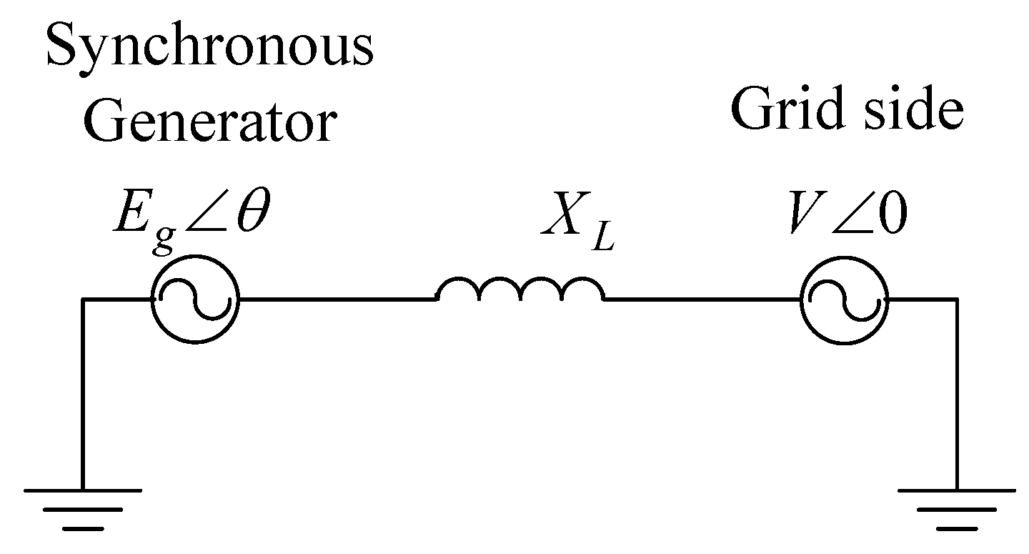
Figure 2.
Active power transferred from the generator to the grid versus angle.
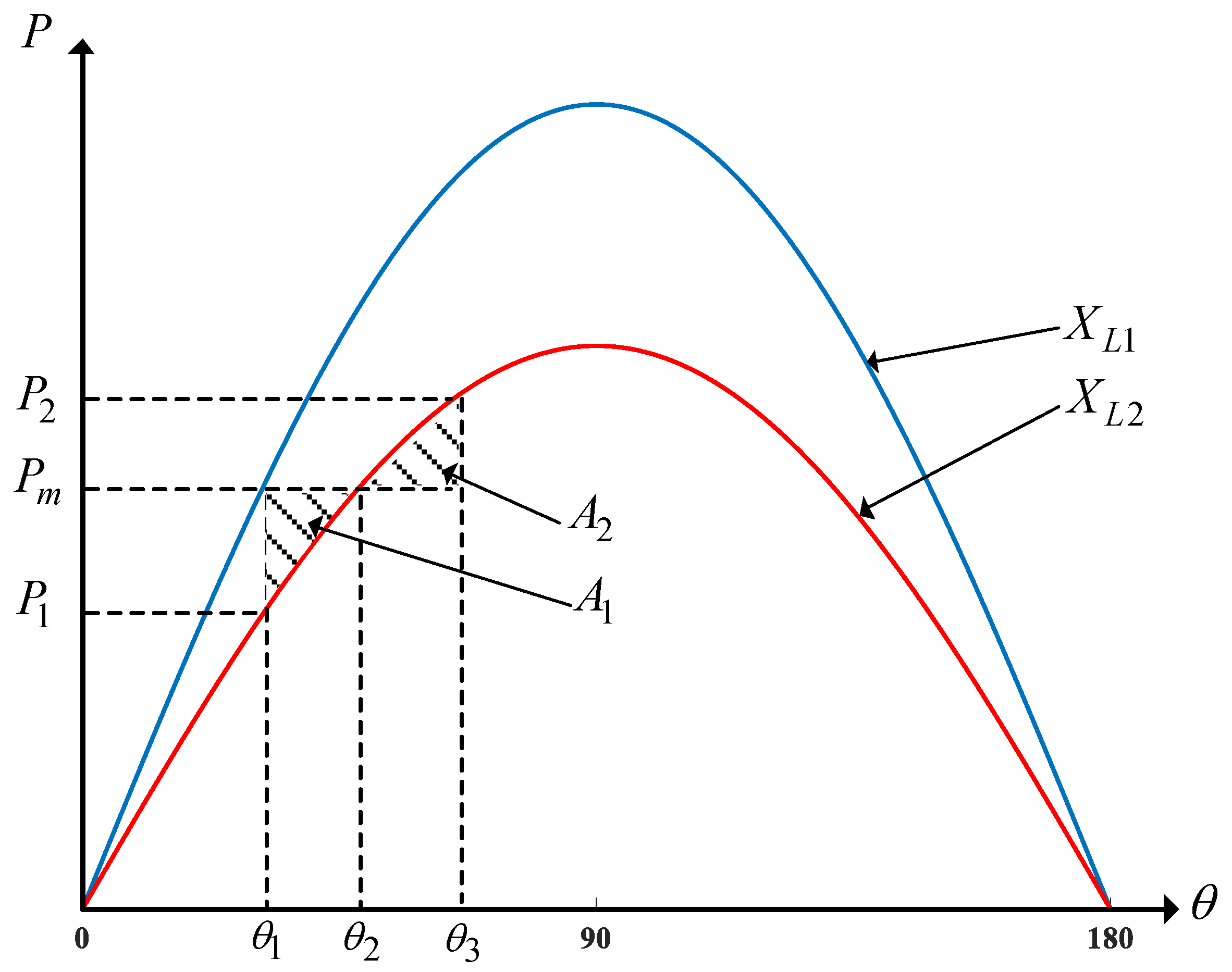
Figure 3.
A Grid-connected VSC working in the grid-feeding mode.

Figure 4.
Block diagram of the used Phase Locked Loop.
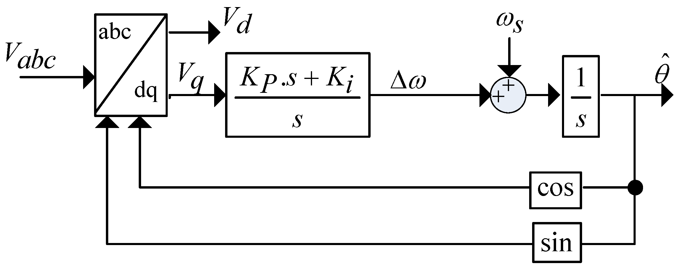
Figure 5.
Block diagram of the grid-connected VSC including the current control and the time delay.

Figure 6.
Eigenvalues of the P matrix for positive values of KP and Ki = 600.
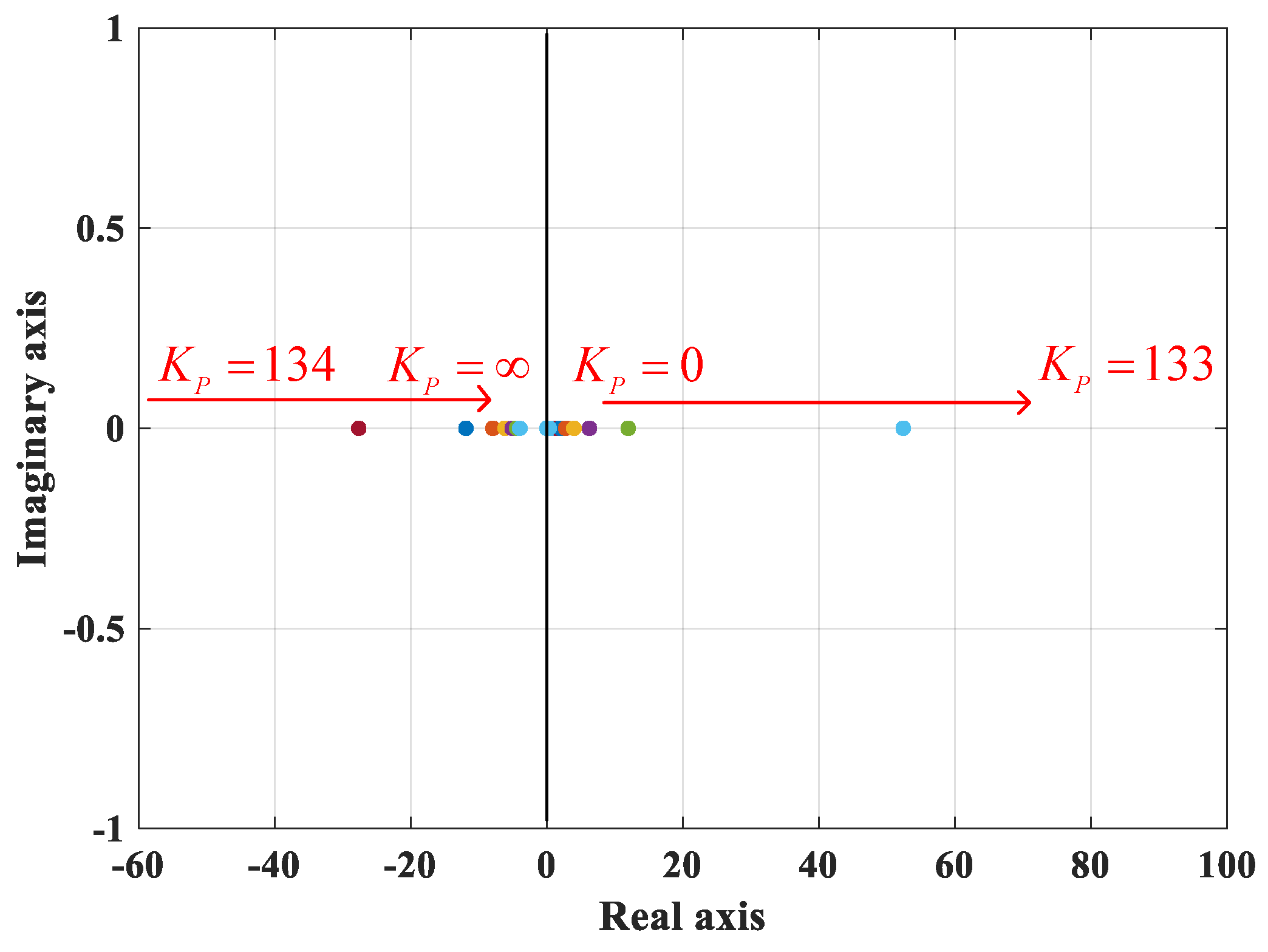
Figure 7.
Eigenvalues of the P matrix for negative values of KP and Ki = 600.

Figure 8.
Lyapunov function of the grid-connected VSC considering different values of the KP and a step change in the reference current at t = 4 s.
Figure 8.
Lyapunov function of the grid-connected VSC considering different values of the KP and a step change in the reference current at t = 4 s.

Figure 9.
The VSC’s output current response to the step change in current reference from 50 A to 75 A at t = 4 s with KP = 40.
Figure 9.
The VSC’s output current response to the step change in current reference from 50 A to 75 A at t = 4 s with KP = 40.
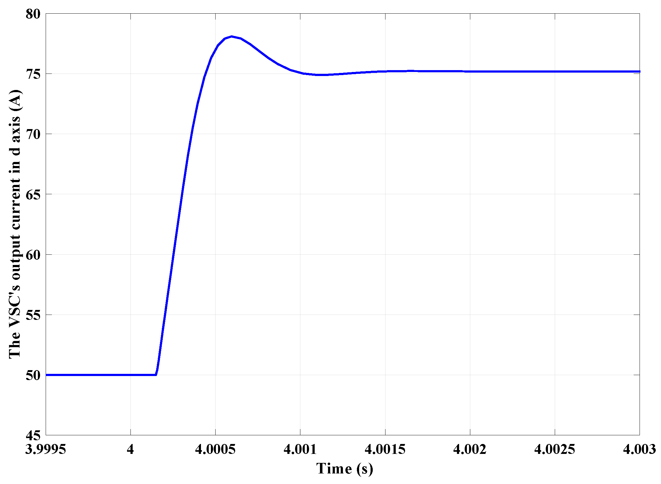
Figure 10.
The energy function of the system with Id.ref = 50 A and change in KP from 70 to 140 at t = 2 s.
Figure 10.
The energy function of the system with Id.ref = 50 A and change in KP from 70 to 140 at t = 2 s.

Figure 11.
The Lyapunov function and the VSC’s output current in d-axis and in the three-phases for a step change in KP value from 80 to 160 at t = 2 s.
Figure 11.
The Lyapunov function and the VSC’s output current in d-axis and in the three-phases for a step change in KP value from 80 to 160 at t = 2 s.

Figure 12.
The Lyapunov function, the VSC’s output current in d-axis and in three-phase, and the grid-side three-phase voltage value for voltage sag at t = 3 s for a period of 1 s and a step change in the current reference from 10 A to 15 A at t = 5 s.
Figure 12.
The Lyapunov function, the VSC’s output current in d-axis and in three-phase, and the grid-side three-phase voltage value for voltage sag at t = 3 s for a period of 1 s and a step change in the current reference from 10 A to 15 A at t = 5 s.
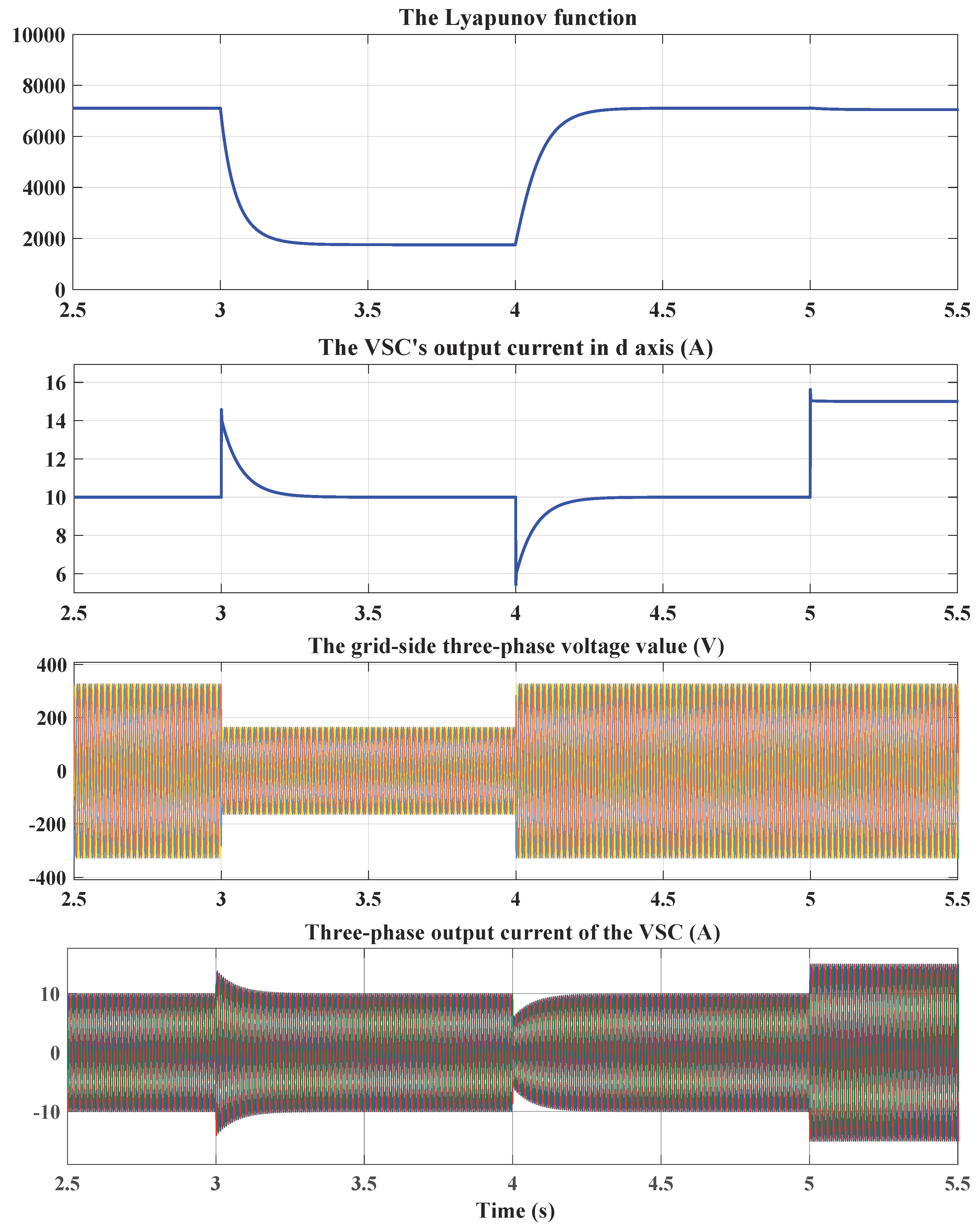
Figure 13.
The three-phase output current of the VSC response to the (a) 50% voltage sag in grid-side voltage magnitude, and (b) step change in current reference from 10 A to 15 A.
Figure 13.
The three-phase output current of the VSC response to the (a) 50% voltage sag in grid-side voltage magnitude, and (b) step change in current reference from 10 A to 15 A.

Table 1.
Power Electronic-based power system stability techniques and their characteristic.
| Power Electronic-Based Power System Stability Assessment | |||
|---|---|---|---|
| Linear-Based Method [5] | Nonlinear-Based Methods [15] | ||
| Techniques | |||
| Characteristic | |||
| Global equilibrium point | Only valid for one equilibrium point | Valid for all equilibrium points | |
| Model accuracy | An approximation of the system will be modeled using linearizaing techniques [28]. | The exact model of the system will be evaluated. | |
| Computation complexity | They are mostly easy to implement and assess. | Nonlinear-based methods are more complex than linear techniques. Their computational burden increase as the system size increases. | |
Table 2.
System parameters for the grid-connected VSC.
| System Parameters | Value | Explanation |
|---|---|---|
| L-filter | 10 mH | The VSC output includes only an L-filter. Alternatively, an LCL filter may be used. |
| Vgrid | 400 V (rms phase to phase) | An ideal voltage source is used as the grid equivalent. |
| System Frequency | 50 Hz | - |
| Controlling system time delay | 1.5 | delay is caused by the computation process and 0.5 is due to the PWM. |
| 10 s | The sampling frequency is chosen to be equal to 10 kHz. |
© 2018 by the authors. Licensee MDPI, Basel, Switzerland. This article is an open access article distributed under the terms and conditions of the Creative Commons Attribution (CC BY) license (http://creativecommons.org/licenses/by/4.0/).
Share and Cite
MDPI and ACS Style
Shakerighadi, B.; Ebrahimzadeh, E.; Blaabjerg, F.; Leth Bak, C. Large-Signal Stability Modeling for the Grid-Connected VSC Based on the Lyapunov Method. Energies 2018, 11, 2533. https://doi.org/10.3390/en11102533
AMA Style
Shakerighadi B, Ebrahimzadeh E, Blaabjerg F, Leth Bak C. Large-Signal Stability Modeling for the Grid-Connected VSC Based on the Lyapunov Method. Energies. 2018; 11(10):2533. https://doi.org/10.3390/en11102533
Chicago/Turabian StyleShakerighadi, Bahram, Esmaeil Ebrahimzadeh, Frede Blaabjerg, and Claus Leth Bak. 2018. "Large-Signal Stability Modeling for the Grid-Connected VSC Based on the Lyapunov Method" Energies 11, no. 10: 2533. https://doi.org/10.3390/en11102533
Note that from the first issue of 2016, this journal uses article numbers instead of page numbers. See further details here.