A Novel Model Incorporating Geomechanics for a Horizontal Well in a Naturally Fractured Reservoir

Abstract

Fracture aperture of a fractured reservoir can be affected by both matrix elasticity and fracture compressibility when the reservoir pressure decreases, namely stress sensitivity. An elasticity parameter coupling Young’s modulus and Poisson’s ratio was introduced to reflect this geomechanical behavior, and a new model incorporating geomechanics was developed to analyze the flow behavior of a horizontal well in a naturally fractured reservoir. Pressure solutions for two cases—uniform-flux and infinite-conductivity—were derived, respectively. For the uniform-flux case, the effect of dimensionless elasticity parameter on the pressure-drop profile becomes stronger with continuing production, and the profile may be like a bow. Nine flow regimes can be observed on the transient response of the infinite-conductivity case. Stress sensitivity mainly affects the late-flow period and a larger dimensionless elasticity parameter causes a greater pressure drop. Due to stress sensitivity, the pressure derivative curve exhibits an upward tendency in the pseudo-radial flow regime, and the slope is greater than “1” in the pseudo-steady flow regime. For KT-I formation in the North Truva field, its elasticity parameter decreases with the increase of Young’s modulus or Poisson’s ratio and ranges from 8 × 10⁻⁸ Pa⁻¹ to 1.1 × 10⁻⁷ Pa⁻¹. Meanwhile, the transient response of H519 has a slight negative correlation with Young’s modulus and Poisson’s ratio in the pseudo-steady flow regime.

1. Introduction

Horizontal wells have been an important technique to improve oil recovery, and naturally fractured reservoirs are one of the potential targets to use this kind of well type [1,2,3,4]. Reservoir pressure depletion in the naturally fractured reservoirs changes the stress balance of reservoir rock and then changes fracture permeability, namely stress sensitivity, which is a typical geomechanical behavior of naturally fractured reservoirs [5,6,7,8,9]. Therefore, it is of great significance to investigate the flow behavior of a horizontal well in the naturally fractured reservoir, especially after a long period of production.

The dual-porosity model, including a natural fracture system and a matrix system, is always used to simulate the fluid flow in a naturally fractured medium [10,11]. The geometric characteristics of natural fractures may vary over a range of scales. They can increase reservoir capacity and conductivity, but also can act like a barrier to fluid flow [12,13]. Based on the characteristics of the dual-porosity model, three classical models are developed to deal with the fluid-flow problems in naturally fractured reservoirs, including the sugar-cube model presented by Warren and Root [14], the slab-shaped matrix model presented by Kazemi [15] and the sphere-shaped matrix model presented by de Swaan [16]. Thus, we can easily further investigate the transient flow of various well types in naturally fractured reservoirs. However, in these models, stress sensitivity is neglected and petrophysical parameters of natural fracture system are considered as static properties during the production, which obviously does not match the characteristics of naturally fractured reservoirs.

As mentioned before, fracture porosity and fracture permeability are variable since they are related to reservoir pressure. Several approaches have been proposed to incorporate geomechanical effects into the simulation and characterization of elastic media in the literature [17,18,19,20,21,22]. Nur and Yilmaz [17] defined a stress sensitivity coefficient to account for permeability variation, and Kikani and Pedrosa [18] further rewrote it as a form of exponential function. This exponential relationship becomes one of the most common expressions and is widely used to describe stress-sensitive reservoirs. On the basis of this relationship, Ceils et al. [23] and Samaniego and Villalobos [24] investigated the effect of stress sensitivity on the transient flow behavior of naturally fractured reservoirs. Similarly, Yao et al. [25] presented a new semi-analytical model for hydraulic fractures with stress-sensitive conductivity, and Zhang et al. [26] also developed an improved model for a finite-conductivity fracture with stress-sensitive fracture permeability. These proposed models highly depend on the exponential relationship between fracture permeability and reservoir pressure. However, stress sensitivity coefficient is mainly obtained by fitting the experimental data measured from the laboratory and it may have a certain error due to the difference between the experimental environment and the actual reservoir conditions [8,17,18]. There are still other approaches to deal with stress sensitivity. Raghavan and Chin [20] established a numerical model coupling geomechanical and fluid-flow aspects to examine the fracture permeability reduction from the partial closure of natural fractures. Rosalind [27] proposed an approach that avoids using pseudo-pressure function to handle stress sensitivity, but this approach is limited to a linear variation of permeability and porosity.

Generally, in terms of stress sensitivity, most proposed models depends on either an exponential relationship or a numerical analysis. Depending on these models, many researchers investigate the transient pressure of vertical wells or fractured wells in stress-sensitive reservoirs [20,23,24,25,26]. However, they do not take the reservoir geomechanical parameters into account. For example, Young’s modulus and Poisson’s ratio, two key parameters reflecting the reservoirs’ geomechanical properties, are not incorporated into these models [28]. By using the theory of geomechanics, Jabbari et al. [22] proposed a fracture permeability model to figure out the dependency of fracture properties on reservoir pressure change, which couples fracture porosity, fracture compressibility, Young’s modulus and Poisson’s ratio. This model provides a completely new method to deal with stress sensitivity and consider geomechanical properties. To be our best knowledge, no research has been done upon horizontal well incorporating nonlinear geomechanics with the model proposed by Jabbari et al. [22], and the corresponding analytical solution for this fluid-flow problem is not available.

The objective of this work was to develop a model incorporating geomechanics for a horizontal well in a naturally fractured reservoir. Firstly, by using a Pedrosa transform, perturbation technique and spatial integral method, analytical pressure solutions for two cases: uniform flux and infinite conductivity, were derived, respectively. Secondly, a special case was employed to verify this uniform-flux pressure solution and the effect of dimensionless elasticity parameter on this horizontal wellbore’s pressure drop profiles was also discussed. Thirdly, based on the infinite-conductivity pressure solution, transient pressure, flow regimes and parameters sensitivity of this model were investigated in detail. Finally, by taking KT-I formation of the North Truva field as an example, the effects of Young’s modulus and Poisson’s ratio of this formation on the elasticity parameter and the transient response of H519 were analyzed.

2. Physical Model

Figure 1 shows a sketch of a horizontal well in a naturally fractured reservoir with stress sensitivity. In order to simplify the mathematical model, basic assumptions are made as follows:

(1)

This formation consists of two systems, including natural fracture system and matrix system, and can be represented by Warren-Root model. Two kinds of porous media are homogeneous, and the closure of natural fractures caused by reservoir pressure depletion is taken into account.

(2)

This reservoir is circular and closed at the external boundary of side and bounded by upper and lower impermeable formation, and has a uniform thickness.

(3)

Flow in this reservoir is considered to be a slightly compressible and single-phase fluid with constant viscosity and obeys Darcy’s law. Pseudo-steady flow from matrix system to natural fracture system is assumed.

(4)

This horizontal well is produced at a constant rate and no fluid is assumed to flow at the tip of the horizontal wellbore.

(5)

Gravity and capillary effects are neglected.

3. Fracture Permeability vs. Mechanical Elasticity

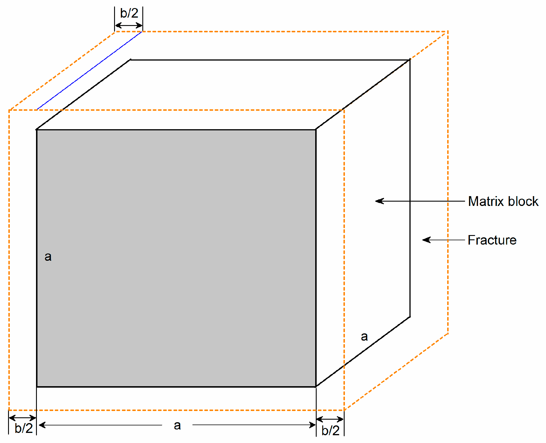
Warren and Root [14] first proposed a sugar-cube model to describe the naturally fractured medium (Figure 2). Based on this conceptual model, we can obtain the fracture porosity for a naturally fractured reservoir:

$${\varphi }_f=\frac{{\left(a+b\right)}^3-a^3}{{\left(a+b\right)}^3}=\frac{3a^{2}b+3a{b}^2+b^3}{a^3+3a^{2}b+3a{b}^2+b^3}$$

(1)

Considering that the fracture aperture is much smaller than the block size, Equation (1) can be approximated as:

$${\varphi }_f\cong \frac{3b}{a}$$

(2)

In the sugar-cube model, assuming that the ratio of fracture width to block height is very small and fluid flows only in y-direction in both the vertical and horizontal fractures, the flow paths in Figure 2 can be approximated by flow through rectangular ducts. Janna [29] proposed the following equation to describe the average velocity of laminar flow through a rectangular duct:

$$\overline{v}=\left(\frac{b^2}{12\mu }\right)\frac{\Delta p}{L}$$

(3)

For a duct, the average velocity also can be described as a function of flow rate and fracture dimensions:

$$\overline{v}=\frac{q}{ab}$$

(4)

Equating Equations (3) and (4), we obtain:

$$q=\frac{a{b}^3\Delta p}{12\mu L}$$

(5)

Thus, the total flow through multiple fractures becomes:

$$Q=nq=\frac{na{b}^3\Delta p}{12\mu L}$$

(6)

Further, Darcy’s Law for linear horizontal flow through a porous medium can be applied:

$$Q=\frac{k_{f}A\Delta p}{\mu L}=\frac{k_{f}n{\left(a+b\right)}^2\Delta p}{\mu L}\cong \frac{k_{f}n{a}^2\Delta p}{\mu L}$$

(7)

Combining Equation (6) with Equation (7), fracture permeability with sugar cube geometry is yielded [22]:

$$k_f=\frac{b^3}{12a}$$

(8)

Obviously, regarding Equation (8), fracture permeability is a stronger function of the fracture width, $b$, than the matrix block size, $a$. Jabbari et al. [22] take the derivative of Equation (8) with respect to reservoir pressure and let fracture width be a function of reservoir pressure, and then obtain the following equation:

$$\frac{d{k}_f}{dp}=\frac{1}{12}\left(\frac{3b^2}{a}\frac{db}{dp}-\frac{b^3}{a^2}\frac{da}{dp}\right)$$

(9)

During the closing of fracture aperture, a positive change in the length of a matrix block corresponds to a negative change in the fracture width, thus, we get a relationship: $\Delta a=-\Delta b$. Substituting this formula into Equation (9), it yields:

$$\frac{d{k}_f}{dp}=\frac{b^2}{4a}\left(1+\frac{b}{3a}\right)\frac{db}{dp}$$

(10)

Jabbari et al. [22] came up with the idea that the total change in fracture width, $\Delta b$, caused by the change of reservoir pressure, is the sum of the change caused by fracture compressibility and matrix elasticity.

On the basis of the general relationship between effective stress, total stress, and fracture pore pressure [30,31], Jabbari et al. [22] presented a formula of the change in fracture width caused by fracture compressibility:

$$\Delta b_f=b{c}_f\Delta p_f$$

(11)

where $\Delta p_f=p-p_i$ is the change in fracture pore pressure.

Similarly, using the theory of geomechanics, Jabbari et al. [22] obtained the change in fracture width that comes from matrix elasticity:

$$\Delta b_m=\frac{a\left(1-2v\right)\Delta p_f}{E}$$

(12)

where $E$ is Young’s modulus, and $v$ is Poisson’s ratio.

Note that as a feasible assumption, the change in overburden pressure is neglected. Hence, the total change in fracture width is:

$$\Delta b_t=\Delta b_f+\Delta b_m-b{c}_f\Delta p_{ob}=\left(b{c}_f+\frac{a\left(1-2v\right)}{E}\right)\Delta p_f-b{c}_f\Delta p_{ob}$$

(13)

where $p_{ob}$ is the overburden pressure.

The differential form of Equation (13) can be written as:

$$db=\left(b{c}_f+\frac{a\left(1-2v\right)}{E}\right)dp-b{c}_{f}d{p}_{ob}$$

(14)

Further, substituting Equation (14) into Equation (10) and neglecting any change in overburden pressure, Jabbari et al. [22] developed an expression of fracture permeability incorporating geomechanics:

$$\frac{d{k}_f}{dp}=\frac{b^3}{4a}\left(1+\frac{{\varphi }_f}{9}\right)\left(c_f\left(1-\frac{d{p}_{ob}}{dp}\right)+\frac{a\left(1-2v\right)}{bE}\right)$$

(15)

If overburden pressure is held constant, Equation (15) is reduced to the following form:

$$\frac{d{k}_f}{dp}=3k_f\left(1+\frac{{\varphi }_f}{9}\right)\left(c_f+\frac{a\left(1-2v\right)}{bE}\right)$$

(16)

Equation (16) is a representation of fracture permeability dependent on reservoir pressure, which considers two significant geomechanical parameters, Young’s modulus and Poisson’s ratio.

4. Point Sink Model in the Closed Cylindrical System

4.1. Mathematical Model in the Closed Cylindrical System

4.1.1. Governing Equations

According to the law of conservation of mass, we can have the continuity equations for natural fracture system and matrix system:

$$\overrightarrow{\nabla }\left(\rho \frac{k_f}{\mu }\overrightarrow{\nabla }{p}_f\right)+q\ast =\frac{\partial \left(\rho {\varphi }_f\right)}{\partial t}$$

(17)

$$-q\ast =\frac{\partial \left(\rho {\varphi }_m\right)}{\partial t}$$

(18)

respectively.

Pseudo-steady flow has been assumed between natural fracture system and matrix system, and the inter-porosity flow equation can be given as:

$$q\ast =\frac{\alpha k_m\rho }{\mu }\left(p_m-p_f\right)$$

(19)

where $\alpha$ is a parameter related to the geometry of natural fractures.

With Equation (19), Equations (17) and (18) can be transformed into:

$$\frac{1}{\rho }\overrightarrow{\nabla }\left(\rho \frac{k_f}{\mu }\overrightarrow{\nabla }{p}_f\right)=\frac{\partial {\varphi }_f}{\partial t}+\frac{\partial {\varphi }_m}{\partial t}$$

(20)

$$-\frac{\alpha k_m}{\mu }\left(p_m-p_f\right)=\frac{\partial {\varphi }_m}{\partial t}$$

(21)

The porosity change of natural fracture and matrix during reservoir production can be described by the following equations, respectively:

$${\varphi }_f={\varphi }_{f0}{e}^{c_f\left(p_f-p_i\right)}$$

(22)

$${\varphi }_m={\varphi }_{m0}{e}^{c_m\left(p_m-p_i\right)}$$

(23)

where ${\varphi }_{f0}$ and ${\varphi }_{m0}$ are the initial porosity of natural fracture system and matrix system; $c_f$ and $c_m$ are the compressibility of natural fracture system and matrix system.

If the connate-water saturation in the matrix medium is assumed to be negligible, we can obtain a reasonable estimate expression of fracture compressibility:

$$c_f=\frac{1}{\rho }\frac{\partial \rho }{\partial p_f}\cong c_o$$

(24)

where $c_o$ is the oil compressibility.

Using Equations (22) and (23), we can obtain:

$$\frac{\partial {\varphi }_f}{\partial t}=\frac{\partial \left({\varphi }_{f0}{e}^{c_f\left(p_f-p_i\right)}\right)}{\partial t}\approx {\varphi }_{f0}{c}_f\frac{\partial p_f}{\partial t}$$

(25)

$$\frac{\partial {\varphi }_m}{\partial t}=\frac{\partial \left({\varphi }_{m0}{e}^{c_m\left(p_m-p_i\right)}\right)}{\partial t}\approx {\varphi }_{m0}{c}_m\frac{\partial p_m}{\partial t}$$

(26)

where ${\varphi }_{f0}{c}_f$ and ${\varphi }_{m0}{c}_m$ are the storage of natural fracture system and matrix system, respectively.

Substituting Equations (25) and (26) into Equations (20) and (21), we have the governing equations for the point sink model in the naturally fractured reservoir:

$$\frac{1}{\rho }\overrightarrow{\nabla }\left(\rho \frac{k_f}{\mu }\overrightarrow{\nabla }{p}_f\right)={\varphi }_{f0}{c}_f\frac{\partial p_f}{\partial t}+{\varphi }_{m0}{c}_m\frac{\partial p_m}{\partial t}$$

(27)

$$-\frac{\alpha k_m}{\mu }\left(p_m-p_f\right)={\varphi }_{m0}{c}_m\frac{\partial p_m}{\partial t}$$

(28)

Considering that fracture permeability depends on reservoir pressure, we can transform the term on the left-hand side of Equation (27) into:

$$\frac{1}{\rho }\overrightarrow{\nabla }\left(\rho \frac{k_f}{\mu }\overrightarrow{\nabla }{p}_f\right)=\frac{k_f}{\mu }{\nabla }^2{p}_f+\frac{1}{\mu }\overrightarrow{\nabla }{k}_f\cdot \overrightarrow{\nabla }{p}_f+\frac{k_f}{\mu \rho }\overrightarrow{\nabla }\rho \cdot \overrightarrow{\nabla }{p}_f$$

(29)

With Equation (16), the second term on the right-hand side of Equation (29) can be rewritten as:

$$\frac{1}{\mu }\overrightarrow{\nabla }{k}_f\cdot \overrightarrow{\nabla }{p}_f=\frac{k_f}{\mu }\left[3\left(1+\frac{{\varphi }_f}{9}\right)\left(c_f+\frac{3\left(1-2\nu \right)}{E{\varphi }_f}\right)\right]\overrightarrow{\nabla }{p}_f\cdot \overrightarrow{\nabla }{p}_f$$

(30)

Similarly, by introducing Equation (24), the last term on the right-hand side of Equation (29) can be further rewritten as:

$$\frac{k_f}{\mu \rho }\overrightarrow{\nabla }\rho \cdot \overrightarrow{\nabla }{p}_f=\frac{k_f}{\mu }\frac{1}{\rho }\frac{\partial \rho }{\partial p_f}\overrightarrow{\nabla }{p}_f\cdot \overrightarrow{\nabla }{p}_f=\frac{k_f}{\mu }{c}_o\overrightarrow{\nabla }{p}_f\cdot \overrightarrow{\nabla }{p}_f$$

(31)

Substituting Equations (30) and (31) into Equation (29), we have:

$$\frac{1}{\rho }\overrightarrow{\nabla }\left(\rho \frac{k_f}{\mu }\overrightarrow{\nabla }{p}_f\right)=\frac{k_f}{\mu }\left\{{\nabla }^2{p}_f+\left[c_o+3\left(1+\frac{{\varphi }_f}{9}\right)\left(c_f+\frac{3\left(1-2\nu \right)}{E{\varphi }_f}\right)\right]\overrightarrow{\nabla }{p}_f\cdot \overrightarrow{\nabla }{p}_f\right\}$$

(32)

To simplify the model derivation, we define a new elasticity parameter:

$$\epsilon =c_o+3\left(1+\frac{{\varphi }_f}{9}\right)\left(c_f+\frac{3\left(1-2\nu \right)}{E{\varphi }_f}\right)$$

(33)

Obviously, this parameter depends on oil compressibility, fracture porosity, fracture compressibility, Young’s modulus and Poisson’s ratio, thus, Equation (32) can be simplified as:

$$\frac{1}{\rho }\overrightarrow{\nabla }\left(\rho \frac{k_f}{\mu }\overrightarrow{\nabla }{p}_f\right)=\frac{k_f}{\mu }\left({\nabla }^2{p}_f+\epsilon \overrightarrow{\nabla }{p}_f\cdot \overrightarrow{\nabla }{p}_f\right)$$

(34)

In the cylindrical coordinate system, we have:

$$\overrightarrow{\nabla }{p}_f=\left(\frac{\partial p_f}{\partial r},\frac{\partial p_f}{\partial z}\right)$$

(35)

$${\nabla }^2{p}_f=\frac{{\partial }^2{p}_f}{\partial r^2}+\frac{1}{r}\frac{\partial p_f}{\partial r}+\frac{{\partial }^2{p}_f}{\partial z^2}$$

(36)

Combining Equations (34)–(36) with Equation (27), the continuity equation for natural fracture system becomes:

$$\frac{k_f}{\mu }\left\{\left(\frac{{\partial }^2{p}_f}{\partial r^2}+\frac{1}{r}\frac{\partial p_f}{\partial r}+\frac{{\partial }^2{p}_f}{\partial z^2}\right)+\epsilon \left[{\left(\frac{\partial p_f}{\partial r}\right)}^2+{\left(\frac{\partial p_f}{\partial z}\right)}^2\right]\right\}={\varphi }_{f0}{c}_f\frac{\partial p_f}{\partial t}+{\varphi }_{m0}{c}_m\frac{\partial p_m}{\partial t}$$

(37)

4.1.2. Initial Conditions and Boundary Conditions

According to the physical model above, we can obtain the corresponding constraint conditions for the point sink model as follows:

Initial conditions:

$$p_f\left(r,z,0\right)=p_m\left(r,z,0\right)=0$$

(38)

Inner boundary condition:

$$\underset{\zeta \to 0}{\lim }\left[\frac{1}{\zeta }\underset{r\to 0}{\lim }{\displaystyle \underset{z_w-\frac{\zeta }{2}}{\overset{z_w+\frac{\zeta }{2}}{\int }}\left(\frac{2\pi k_f}{\mu B}r\frac{\partial p_f}{\partial r}\right)dz}\right]=q_{po\mathrm{int}}\left(t\right)$$

(39)

where $q_{po\mathrm{int}}\left(t\right)$ is the production rate of point sink.

Outer boundary condition:

$${\frac{\partial p_f}{\partial r}|}_{r=r_e}=0$$

(40)

Upper and lower boundary conditions:

$${\frac{\partial p_f}{\partial z}|}_{z=0}={\frac{\partial p_f}{\partial z}|}_{z=h}=0$$

(41)

In the cylindrical system, Equations (28) and (37)–(41) compose a point sink model incorporating geomechanical property in the naturally fractured reservoir.

4.2. Point Sink Model Solution

In order to unify and solve the model easily, the dimensionless variables defined in

Table 1. Definitions of dimensionless variables.

Parameters	Definitions
Dimensionless time	$t_D=\frac{k_{f}t}{\mu \left[{\varphi }_{f0}{c}_f+{\varphi }_{m0}{c}_m\right]r_w^2}$
Dimensionless pressure	$p_{jD}=\frac{2\pi k_{f}h\left(p_i-p_j\right)}{q\mu B}$
Dimensionless x-, y-, z-coordinate	$x_D=\frac{x}{L}$, $y_D=\frac{y}{L}$, $z_D=\frac{z}{h}$
Dimensionless x-, y-, z-coordinate of wellbore	$x_{wD}=\frac{x_w}{L}$, $y_{wD}=\frac{y_w}{L}$, $z_{wD}=\frac{z_w}{h}$
Dimensionless radius distance	$r_D=\frac{r}{L}=\sqrt{x_D^2+y_D^2}$
Dimensionless wellbore radius	$r_{wD}=\frac{r_w}{L}$
Dimensionless reservoir boundary radius	$r_{eD}=\frac{r_e}{L}$
Dimensionless z-coordinate of wellbore	$z_{wD}=\frac{z_w}{h}$
Dimensionless wellbore length	$L_D=\frac{L}{h}$
Dimensionless reservoir thickness	$h_D=\frac{h}{r_w}$
Dimensionless infinitesimal vertical distance	${\zeta }_D=\frac{\zeta }{h}$
Dimensionless elasticity parameter	${\epsilon }_D=\frac{q\mu B}{2\pi k_{f}h}\epsilon$
Interporosity flow coefficient	$\lambda =\frac{\alpha k_m{r}_w^2}{k_f}$
Fracture storage capacity	$\omega =\frac{{\varphi }_{f0}{c}_f}{{\varphi }_{f0}{c}_f+{\varphi }_{m0}{c}_m}$
Dimensionless production rate of point sink	$q_{po\mathrm{int}D}\left(t_D\right)=\frac{q_{po\mathrm{int}}\left(t\right)}{q}$
Dimensionless wellbore storage coefficient	$C_D=\frac{C}{2\pi h\left({\varphi }_{f0}{c}_f+{\varphi }_{m0}{c}_m\right)r_w^2}$
Skin factor	$S=\frac{2\pi k_{f}h}{q\mu B}\Delta p_s$

where $r_{wD}{L}_D{h}_D=1$.

are used to deal with the above equations.

Based on these dimensionless variables, Equations (28) and (37)–(41) can be transformed into the following dimensionless forms:

Governing equations:

$$\frac{{\partial }^2{p}_{fD}}{\partial r_D^2}+\frac{1}{r_D}\frac{\partial p_{fD}}{\partial r_D}+L_D^2\frac{{\partial }^2{p}_{fD}}{\partial z_D^2}-{\epsilon }_D\left[{\left(\frac{\partial p_{fD}}{\partial r_D}\right)}^2+L_D^2{\left(\frac{\partial p_{fD}}{\partial z_D}\right)}^2\right]={\left(L_D{h}_D\right)}^2\left[\omega \frac{\partial p_{fD}}{\partial t_D}+\left(1-\omega \right)\frac{\partial p_{mD}}{\partial t_D}\right]$$

(42)

$$-\lambda \left(p_{mD}-p_{fD}\right)=\left(1-\omega \right)\frac{\partial p_{mD}}{\partial t_D}$$

(43)

Initial conditions:

$$p_{fD}\left(r_D,z_D,0\right)=p_{mD}\left(r_D,z_D,0\right)=0$$

(44)

Inner boundary condition:

$$\underset{{\zeta }_D\to 0}{\lim }\left[\frac{1}{{\zeta }_D}\underset{r_D\to 0}{\lim }{\displaystyle \underset{z_{wD}-\frac{{\zeta }_D}{2}}{\overset{z_{wD}+\frac{{\zeta }_D}{2}}{\int }}\left(r_D\frac{\partial p_{fD}}{\partial r_D}\right)d{z}_D}\right]=-q_{po\mathrm{int}D}\left(t_D\right)$$

(45)

Outer boundary condition:

$${\frac{\partial p_{fD}}{\partial r_D}|}_{r_D=r_{eD}}=0$$

(46)

Upper and lower boundary conditions:

$${\frac{\partial p_{fD}}{\partial z_D}|}_{z_D=0}{=\frac{\partial p_{fD}}{\partial z_D}|}_{z_D=1}=0$$

(47)

4.2.1. Pedrosa Transform and Perturbation Transform

Due to the consideration of geomechanics in the governing equation, Equation (42), we obtain a strong nonlinear differential system in the cylindrical system, which causes difficulty in solving the above point sink model. Here we take Pedrosa transform to weaken the strong nonlinearity in Equation (42) and further apply the perturbation theory in this case to obtain an approximate solution. Pedrosa [32] provided a useful transform to deal with the nonlinear equation:

$$p_{fD}=-\frac{1}{{\epsilon }_D}\ln \left[1-{\epsilon }_D{\psi }_{fD}\left(r_D,z_D,t_D\right)\right]$$

(48)

Using Equation (48), we can obtain a series of differential relationships in the cylindrical system as follows:

$$\frac{\partial p_{fD}}{\partial r_D}=\frac{\partial p_{fD}}{\partial {\psi }_{fD}}\frac{\partial {\psi }_{fD}}{\partial r_D}=\frac{1}{1-{\epsilon }_D{\psi }_{fD}}\frac{\partial {\psi }_{fD}}{\partial r_D}$$

(49)

$$\frac{\partial p_{fD}}{\partial t_D}=\frac{1}{1-{\epsilon }_D{\psi }_{fD}}\frac{\partial {\psi }_{fD}}{\partial t_D}$$

(50)

$$\frac{{\partial }^2{p}_{fD}}{\partial r_D^2}=\frac{{\epsilon }_D}{{\left(1-{\epsilon }_D{\psi }_{fD}\right)}^2}{\left(\frac{\partial {\psi }_{fD}}{\partial r_D}\right)}^2+\frac{1}{1-{\epsilon }_D{\psi }_{fD}}\frac{{\partial }^2{\psi }_{fD}}{\partial r_D^2}$$

(51)

$$\frac{\partial p_{fD}}{\partial z_D}=\frac{1}{1-{\epsilon }_D{\psi }_{fD}}\frac{\partial {\psi }_{fD}}{\partial z_D}$$

(52)

$$\frac{{\partial }^2{p}_{fD}}{\partial z_D^2}=\frac{{\epsilon }_D}{{\left(1-{\epsilon }_D{\psi }_{fD}\right)}^2}{\left(\frac{\partial {\psi }_{fD}}{\partial z_D}\right)}^2+\frac{1}{1-{\epsilon }_D{\psi }_{fD}}\frac{{\partial }^2{\psi }_{fD}}{\partial z_D^2}$$

(53)

Substituting Equations (48)–(53) into Equations (42)–(47), we have:

$$\frac{{\partial }^2{\psi }_{fD}}{\partial r_D^2}+\frac{1}{r_D}\frac{\partial {\psi }_{fD}}{\partial r_D}+L_D^2\frac{{\partial }^2{\psi }_{fD}}{\partial z_D^2}={\left(L_D{h}_D\right)}^2\left[\omega \frac{\partial {\psi }_{fD}}{\partial t_D}+\left(1-{\epsilon }_D{\psi }_{fD}\right)\left(1-\omega \right)\frac{\partial p_{mD}}{\partial t_D}\right]$$

(54)

$$-\lambda \left(p_{mD}-p_{fD}\right)=\left(1-\omega \right)\frac{\partial p_{mD}}{\partial t_D}$$

(55)

$${\psi }_{fD}\left(r_D,z_D,0\right)=p_{mD}\left(r_D,z_D,0\right)=0$$

(56)

$$\underset{{\zeta }_D\to 0}{\lim }\left[\frac{1}{{\zeta }_D}\underset{r_D\to 0}{\lim }{\displaystyle \underset{z_{wD}-\frac{{\zeta }_D}{2}}{\overset{z_{wD}+\frac{{\zeta }_D}{2}}{\int }}\left(r_D\frac{1}{1-{\epsilon }_D{\psi }_{fD}}\frac{\partial {\psi }_{fD}}{\partial r_D}\right)d{z}_D}\right]=-q_{po\mathrm{int}D}\left(t_D\right)$$

(57)

$${\frac{\partial {\psi }_{fD}}{\partial r_D}|}_{r_D=r_{eD}}=0$$

(58)

$${\frac{\partial {\psi }_{fD}}{\partial z_D}|}_{z_D=0}{=\frac{\partial {\psi }_{fD}}{\partial z_D}|}_{z_D=1}=0$$

(59)

The strong nonlinearity in Equation (42) is substantially weakened in Equation (54), and by taking perturbation transform [33,34], we can have the approximation of point sink model’s full solution:

$${\psi }_{fD}={\psi }_{fD0}+{\epsilon }_D{\psi }_{fD1}+{\epsilon }_D^2{\psi }_{fD2}+\cdots$$

(60)

For small ${\epsilon }_D$, these higher-order terms in the series become successively smaller and the zero-order perturbation solution can satisfy the accuracy requirement. Then, Equations (54)–(59) can be transformed into:

$$\frac{{\partial }^2{\psi }_{fD0}}{\partial r_D^2}+\frac{1}{r_D}\frac{\partial {\psi }_{fD0}}{\partial r_D}+L_D^2\frac{{\partial }^2{\psi }_{fD0}}{\partial z_D^2}={\left(L_D{h}_D\right)}^2\left[\omega \frac{\partial {\psi }_{fD0}}{\partial t_D}+\left(1-\omega \right)\frac{\partial p_{mD}}{\partial t_D}\right]$$

(61)

$$-\lambda \left(p_{mD}-p_{fD}\right)=\left(1-\omega \right)\frac{\partial p_{mD}}{\partial t_D}$$

(62)

$${\psi }_{fD0}\left(r_D,z_D,0\right)=p_{mD}\left(r_D,z_D,0\right)=0$$

(63)

$$\underset{{\zeta }_D\to 0}{\lim }\left[\frac{1}{{\zeta }_D}\underset{r_D\to 0}{\lim }{\displaystyle \underset{z_{wD}-\frac{{\zeta }_D}{2}}{\overset{z_{wD}+\frac{{\zeta }_D}{2}}{\int }}\left(r_D\frac{\partial {\psi }_{fD0}}{\partial r_D}\right)d{z}_D}\right]=-q_{po\mathrm{int}D}\left(t_D\right)$$

(64)

$${\frac{\partial {\psi }_{fD0}}{\partial r_D}|}_{r_D=r_{eD}}=0$$

(65)

$${\frac{\partial {\psi }_{fD0}}{\partial z_D}|}_{z_D=0}{=\frac{\partial {\psi }_{fD0}}{\partial z_D}|}_{z_D=1}=0$$

(66)

4.2.2. Laplace Transform and Fourier Transform

By employing a Laplace transform of Equations (61)–(66) with respect to $t_D$, we can obtain the following equations in the Laplace domain:

$$\frac{{\partial }^2{\tilde{\psi }}_{fD0}}{\partial r_D^2}+\frac{1}{r_D}\frac{\partial {\tilde{\psi }}_{fD0}}{\partial r_D}+L_D^2\frac{{\partial }^2{\tilde{\psi }}_{fD0}}{\partial z_D^2}=s{\left(L_D{h}_D\right)}^2\left[\omega {\tilde{\psi }}_{fD0}+\left(1-\omega \right){\tilde{p}}_{mD}\right]$$

(67)

$$-\lambda \left({\tilde{p}}_{mD}-{\tilde{p}}_{fD}\right)=\left(1-\omega \right)s{\tilde{p}}_{mD}$$

(68)

$$\underset{{\zeta }_D\to 0}{\lim }\left[\frac{1}{{\zeta }_D}\underset{r_D\to 0}{\lim }{\displaystyle \underset{z_{wD}-\frac{{\zeta }_D}{2}}{\overset{z_{wD}+\frac{{\zeta }_D}{2}}{\int }}\left(r_D\frac{\partial {\tilde{\psi }}_{fD0}}{\partial r_D}\right)d{z}_D}\right]=-{\tilde{q}}_{po\mathrm{int}D}\left(s\right)$$

(69)

$${\frac{\partial {\tilde{\psi }}_{fD0}}{\partial r_D}|}_{r_D=r_{eD}}=0$$

(70)

$${\frac{\partial {\tilde{\psi }}_{fD0}}{\partial z_D}|}_{z_D=0}{=\frac{\partial {\tilde{\psi }}_{fD0}}{\partial z_D}|}_{z_D=1}=0$$

(71)

Combining Equation (67) with Equation (68), we can obtain:

$$\frac{{\partial }^2{\tilde{\psi }}_{fD0}}{\partial r_D^2}+\frac{1}{r_D}\frac{\partial {\tilde{\psi }}_{fD0}}{\partial r_D}+L_D^2\frac{{\partial }^2{\tilde{\psi }}_{fD0}}{\partial z_D^2}=s{\left(L_D{h}_D\right)}^2\left[\omega {\tilde{\psi }}_{fD0}+\frac{\left(1-\omega \right)\lambda }{\left(1-\omega \right)s+\lambda }{\tilde{p}}_{fD}\right]$$

(72)

Applying the Taylor series expansion to Equation (48), it becomes:

$$p_{fD}=-\frac{1}{{\epsilon }_D}\ln \left[1-{\epsilon }_D{\psi }_{fD}\left(r_D,z_D,t_D\right)\right]={\psi }_{fD}+\frac{1}{2}{\epsilon }_D{\psi }_{fD}^2+\cdots$$

(73)

Similarly, for small ${\epsilon }_D$ the zero-order perturbation solution can satisfy the accuracy requirement, thus, we have in Laplace domain:

$${\tilde{p}}_{fD}\approx {\tilde{\psi }}_{fD0}$$

(74)

Substituting Equation (74) into Equation (72), the governing equation can be simplified as:

$$\frac{{\partial }^2{\tilde{\psi }}_{fD0}}{\partial r_D^2}+\frac{1}{r_D}\frac{\partial {\tilde{\psi }}_{fD0}}{\partial r_D}+L_D^2\frac{{\partial }^2{\tilde{\psi }}_{fD0}}{\partial z_D^2}=sf\left(s\right){\left(L_D{h}_D\right)}^2{\tilde{\psi }}_{fD0}$$

(75)

where $f\left(s\right)=\frac{\omega \left(1-\omega \right)s+\lambda }{\left(1-\omega \right)s+\lambda }$.

Equations (69)–(71) and (75) compose the zero-order mathematical model of a point sink in the naturally fractured reservoir in Laplace domain. Essentially, this zero-order model is the same as the conventional point-source model in the closed cylindrical system presented by Ozkan [2].

In order to obtain the zero-order point sink solution, we can take the following finite Fourier cosine transform with respect to $z_D$ for this model:

$$F\left[{\tilde{\psi }}_{fD0}\left(r_D,z_D,s\right)\right]={\overline{\tilde{\psi }}}_{fD0}\left(r_D,n,s\right)={\displaystyle \underset{0}{\overset{1}{\int }}{\tilde{\psi }}_{fD0}\left(r_D,z_D,s\right)\cos \left(n\pi z_D\right)d{z}_D}$$

(76)

The inverse of this finite Fourier cosine transform with respect to $z_D$ is:

$$F^{-1}\left[{\overline{\tilde{\psi }}}_{fD0}\left(r_D,n,s\right)\right]={\tilde{\psi }}_{fD0}\left(r_D,z_D,s\right)={\displaystyle \sum _{n=0}^{\infty }\frac{\cos \left(n\pi z_D\right)}{N\left(n\right)}{\overline{\tilde{\psi }}}_{fD0}\left(r_D,n,s\right)}$$

(77)

where $N\left(n\right)={\displaystyle \underset{0}{\overset{1}{\int }}{\cos }^2\left(n\pi z_D\right)d{z}_D}=\{\begin{array}{cc}1,& n=0\\ 1/2& n\ne 0\end{array}$.

Applying the finite Fourier cosine transform to Equation (75) and combining with Equation (71), we obtain:

$$\frac{{\partial }^2{\overline{\tilde{\psi }}}_{fD0}}{\partial r_D^2}+\frac{1}{r_D}\frac{\partial {\overline{\tilde{\psi }}}_{fD0}}{\partial r_D}=\left[sf\left(s\right){\left(L_D{h}_D\right)}^2+n^2{\pi }^2{L}_D^2\right]{\overline{\tilde{\psi }}}_{fD0}$$

(78)

Similarly, taking a Fourier transform for the boundary conditions, Equations (69) and (70) become:

$$\underset{{\zeta }_D\to 0}{\lim }{\left(r_D\frac{\partial {\overline{\tilde{\psi }}}_{fD0}}{\partial r_D}\right)}_{r_D={\zeta }_D}=-{\tilde{q}}_{po\mathrm{int}D}\left(s\right)\cos \left(n\pi z_{wD}\right)$$

(79)

$${\frac{\partial {\overline{\tilde{\psi }}}_{fD0}}{\partial r_D}|}_{r_D=r_{eD}}=0$$

(80)

4.2.3. Model Solution

The governing equation, Equation (78), is a modified Bessel equation. Combining with Equations (78)–(80), the general solution for the zero-order point sink model can be obtained:

$${\overline{\tilde{\psi }}}_{fD0}\left(r_D,n,s\right)={\tilde{q}}_{po\mathrm{int}D}\left(s\right)\cos \left(n\pi z_{wD}\right)\left[K_0\left(\sqrt{u_n}{r}_D\right)+\frac{K_1\left(\sqrt{u_n}{r}_{eD}\right)}{I_1\left(\sqrt{u_n}{r}_{eD}\right)}{I}_0\left(\sqrt{u_n}{r}_D\right)\right]$$

(81)

where $u_n=sf\left(s\right){\left(L_D{h}_D\right)}^2+n^2{\pi }^2{L}_D^2$, $n=0,1,2\cdots$.

With the inverse of finite Fourier cosine transform given by Equation (77), the general solution of a point sink in Laplace domain can be expressed as:

$$\begin{array}{l}{\tilde{\psi }}_{fD}\left(r_D,z_D,s\right)={\tilde{\psi }}_{fD0}\left(r_D,z_D,s\right)={\tilde{q}}_{po\mathrm{int}D}\left(s\right)\{K_0\left(\sqrt{u_0}{r}_D\right)+\frac{K_1\left(\sqrt{u_0}{r}_{eD}\right)}{I_1\left(\sqrt{u_0}{r}_{eD}\right)}{I}_0\left(\sqrt{u_0}{r}_D\right)\\ +2{\displaystyle \sum _{n=1}^{\infty }\left[\cos \left(n\pi z_D\right)\cos \left(n\pi z_{wD}\right)\left(K_0\left(\sqrt{u_n}{r}_D\right)+\frac{K_1\left(\sqrt{u_n}{r}_{eD}\right)}{I_1\left(\sqrt{u_n}{r}_{eD}\right)}{I}_0\left(\sqrt{u_n}{r}_D\right)\right)\right]}\}\end{array}$$

(82)

Equation (82) is the point sink model solution in the closed cylindrical system. As shown in Figure 1, the horizontal wellbore is deployed along the x-axis ($y_{wD}=0$), so we can get the following relationship: $r_D=\sqrt{{\left(x_D-x_{wD}\right)}^2+y_D^2}$. Further, substituting this relationship into Equation (82), we can rewrite it as:

$$\begin{array}{l}{\tilde{\psi }}_{fD}\left(x_D,y_D,z_D,x_{wD},z_{wD},r_{eD},h_D,L_D,s\right)={\tilde{q}}_{po\mathrm{int}D}\left(s\right)\{K_0\left(\sqrt{u_0}\sqrt{{\left(x_D-x_{wD}\right)}^2+y_D^2}\right)+\frac{K_1\left(\sqrt{u_0}{r}_{eD}\right)}{I_1\left(\sqrt{u_0}{r}_{eD}\right)}{I}_0\left(\sqrt{u_0}\sqrt{{\left(x_D-x_{wD}\right)}^2+y_D^2}\right)\\ +2{\displaystyle \sum _{n=1}^{\infty }\left[\cos \left(n\pi z_D\right)\cos \left(n\pi z_{wD}\right)\left(K_0\left(\sqrt{u_n}\sqrt{{\left(x_D-x_{wD}\right)}^2+y_D^2}\right)+\frac{K_1\left(\sqrt{u_n}{r}_{eD}\right)}{I_1\left(\sqrt{u_n}{r}_{eD}\right)}{I}_0\left(\sqrt{u_n}\sqrt{{\left(x_D-x_{wD}\right)}^2+y_D^2}\right)\right)\right]}\}\end{array}$$

(83)

5. Horizontal Well Model Incorporating Geomechanics

When fluid flow along the horizontal wellbore is uniform, by integrating with respect to $x_{wD}$ from −1 to 1 in Equation (83) and letting $y_D=0$ and $z_D=z_{wD}+r_{wD}{L}_D$ [2,35,36], we can obtain the pressure distribution along the horizontal wellbore face in the naturally fractured reservoir:

$$\begin{array}{l}s{\tilde{\psi }}_{HWfD}^{UFFLX}\left(x_D,z_{wD},r_{eD},h_D,L_D,s\right)=\frac{1}{2}\left[{\displaystyle \underset{-1}{\overset{1}{\int }}{K}_0\left(\sqrt{u_0}\left|x_D-x_{wD}\right|\right)d{x}_{wD}}+\frac{K_1\left(\sqrt{u_0}{r}_{eD}\right)}{I_1\left(\sqrt{u_0}{r}_{eD}\right)}{\displaystyle \underset{-1}{\overset{1}{\int }}{I}_0\left(\sqrt{u_0}\left|x_D-x_{wD}\right|\right)d{x}_{wD}}\right]\\ +{\displaystyle \sum _{n=1}^{\infty }\left[\cos \left(n\pi \left(z_{wD}+r_{wD}{L}_D\right)\right)\cos \left(n\pi z_{wD}\right)\left({\displaystyle \underset{-1}{\overset{1}{\int }}{K}_0\left(\sqrt{u_n}\left|x_D-x_{wD}\right|\right)d{x}_{wD}}+\frac{K_1\left(\sqrt{u_n}{r}_{eD}\right)}{I_1\left(\sqrt{u_n}{r}_{eD}\right)}{\displaystyle \underset{-1}{\overset{1}{\int }}{I}_0\left(\sqrt{u_n}\left|x_D-x_{wD}\right|\right)d{x}_{wD}}\right)\right]}\end{array}$$

(84)

Due to the assumption of uniform flux, the pressure along the horizontal wellbore is not uniform and changes with the position and time. To represent the pressure behavior of a horizontal wellbore, no pressure drop in its interior is always assumed, which means that pressure is uniform along the wellbore, and this kind of well is said to have infinite conductivity. This inner-boundary condition poses a very difficult boundary-value problem. Generally, the infinite-conductivity solution can be obtained by selecting a fixed point along the wellbore in the corresponding uniform-flux solution. Clonts and Ramey [37] proposed that the uniform-flux solution with a dimensionless distance of 0.732 was a good approximation of the infinite-conductivity case, and this fixed point was taken by Ozkan [2] to evaluate the pressure for the infinite-conductivity horizontal well. However, the uniform-flux solution at a dimensionless distance of 0.7 or 0.68, presented by Daviau et al. [38] and Rosa and de Carvalho [4], is also used to simulate the flow behavior of infinite-conductivity horizontal well. Therefore, there is no definite result on the selection of the fixed point at present. In this study, the pressure averaging technique based on the uniform-flux solution, proposed by Kuchuk et al. [39], was used to approximate the infinite-conductivity solution. Firstly, integrate along the horizontal wellbore (x-axis) with respect to $x_D$ from −1 to 1 in Equation (84). Then, divide the integral result by the dimensionless wellbore length. Finally, we obtain an average wellbore pressure for the infinite-conductivity horizontal well:

$$\begin{array}{l}s{\tilde{\psi }}_{HWfD}^{INFCD}\left(z_{wD},r_{eD},h_D,L_D,s\right)=\frac{1}{4}{\displaystyle \underset{-1}{\overset{1}{\int }}{\displaystyle \underset{-1}{\overset{1}{\int }}{K}_0\left(\sqrt{u_0}\left|x_D-x_{wD}\right|\right)d{x}_{wD}}+\frac{K_1\left(\sqrt{u_0}{r}_{eD}\right)}{I_1\left(\sqrt{u_0}{r}_{eD}\right)}{\displaystyle \underset{-1}{\overset{1}{\int }}{I}_0\left(\sqrt{u_0}\left|x_D-x_{wD}\right|\right)d{x}_{wD}d{x}_D}}\\ +\frac{1}{2}{\displaystyle \sum _{n=1}^{\infty }\left[\cos \left(n\pi \left(z_{wD}+r_{wD}{L}_D\right)\right)\cos \left(n\pi z_{wD}\right){\displaystyle \underset{-1}{\overset{1}{\int }}{\displaystyle \underset{-1}{\overset{1}{\int }}{K}_0\left(\sqrt{u_n}\left|x_D-x_{wD}\right|\right)d{x}_{wD}}+\frac{K_1\left(\sqrt{u_n}{r}_{eD}\right)}{I_1\left(\sqrt{u_n}{r}_{eD}\right)}{\displaystyle \underset{-1}{\overset{1}{\int }}{I}_0\left(\sqrt{u_n}\left|x_D-x_{wD}\right|\right)d{x}_{wD}}d{x}_D}\right]}\end{array}$$

(85)

Further, the effects of wellbore storage and skin can be easily incorporated into the uniform-flux solution (Equation (84)) and the infinite-conductivity solution (Equation (85)), and we can get the following expressions [40,41]:

$${\tilde{\psi }}_{HWfDSS}^{UFFLX}\left(x_D,y_D,z_D,z_{wD},r_{eD},h_D,L_D,C_D,S,s\right)=\frac{s{\tilde{\psi }}_{HWfD}^{UFFLX}\left(x_D,y_D,z_D,z_{wD},r_{eD},h_D,L_D,s\right)+S}{s\left\{1+s{C}_D\left[s{\tilde{\psi }}_{HWfD}^{UFFLX}\left(x_D,y_D,z_D,z_{wD},r_{eD},h_D,L_D,s\right)+S\right]\right\}}$$

(86)

and:

$${\tilde{\psi }}_{HWfDSS}^{INFCD}\left(z_{wD},r_{eD},h_D,L_D,C_D,S,s\right)=\frac{s{\tilde{\psi }}_{HWfD}^{INFCD}\left(z_{wD},r_{eD},h_D,L_D,s\right)+S}{s\left\{1+s{C}_D\left[s{\tilde{\psi }}_{HWfD}^{INFCD}\left(z_{wD},r_{eD},h_D,L_D,s\right)+S\right]\right\}}$$

(87)

respectively.

By applying the Stehfest numerical algorithm [42] to Equations (86) and (87), the pressure solution in real domain can be obtained. Then, with Pedrosa transform, Equation (48), we can get the pressure response, including the uniform-flux and infinite-conductivity case, for a horizontal well incorporating geomechanics in the naturally fractured reservoir:

$$p_{HWfDSS}^{UFFLX}\left(x_D,z_{wD},r_{eD},h_D,L_D,C_D,S,{\epsilon }_D,t_D\right)=-\frac{1}{{\epsilon }_D}\ln \left[1-{\epsilon }_D{\psi }_{HWfDSS}^{UFFLX}\left(x_D,z_{wD},r_{eD},h_D,L_D,C_D,S,t_D\right)\right]$$

(88)

and:

$$p_{HWfDSS}^{INFCD}\left(z_{wD},r_{eD},h_D,L_D,C_D,S,{\epsilon }_D,t_D\right)=-\frac{1}{{\epsilon }_D}\ln \left[1-{\epsilon }_D{\psi }_{HWfDSS}^{INFCD}\left(z_{wD},r_{eD},h_D,L_D,C_D,S,t_D\right)\right]$$

(89)

According to the definition of dimensionless elasticity parameter ${\epsilon }_D$, when ${\epsilon }_D=0$ it means no consideration of stress sensitivity in the model. We can obtain the pressure solution under this condition by calculating the limit in Equations (88) and (89) as ${\epsilon }_D$ approaches zero:

$$p_{HWfDSS}^{UFFLX}\left(x_D,z_{wD},r_{eD},h_D,L_D,C_D,S,{\epsilon }_D=0,t_D\right)={\psi }_{HWfDSS}^{UFFLX}\left(x_D,z_{wD},r_{eD},h_D,L_D,C_D,S,t_D\right)$$

(90)

and:

$$p_{HWfDSS}^{INFCD}\left(z_{wD},r_{eD},h_D,L_D,C_D,S,{\epsilon }_D=0,t_D\right)={\psi }_{HWfDSS}^{INFCD}\left(z_{wD},r_{eD},h_D,L_D,C_D,S,t_D\right)$$

(91)

6. Results and Discussion

6.1. Verification of the Solution

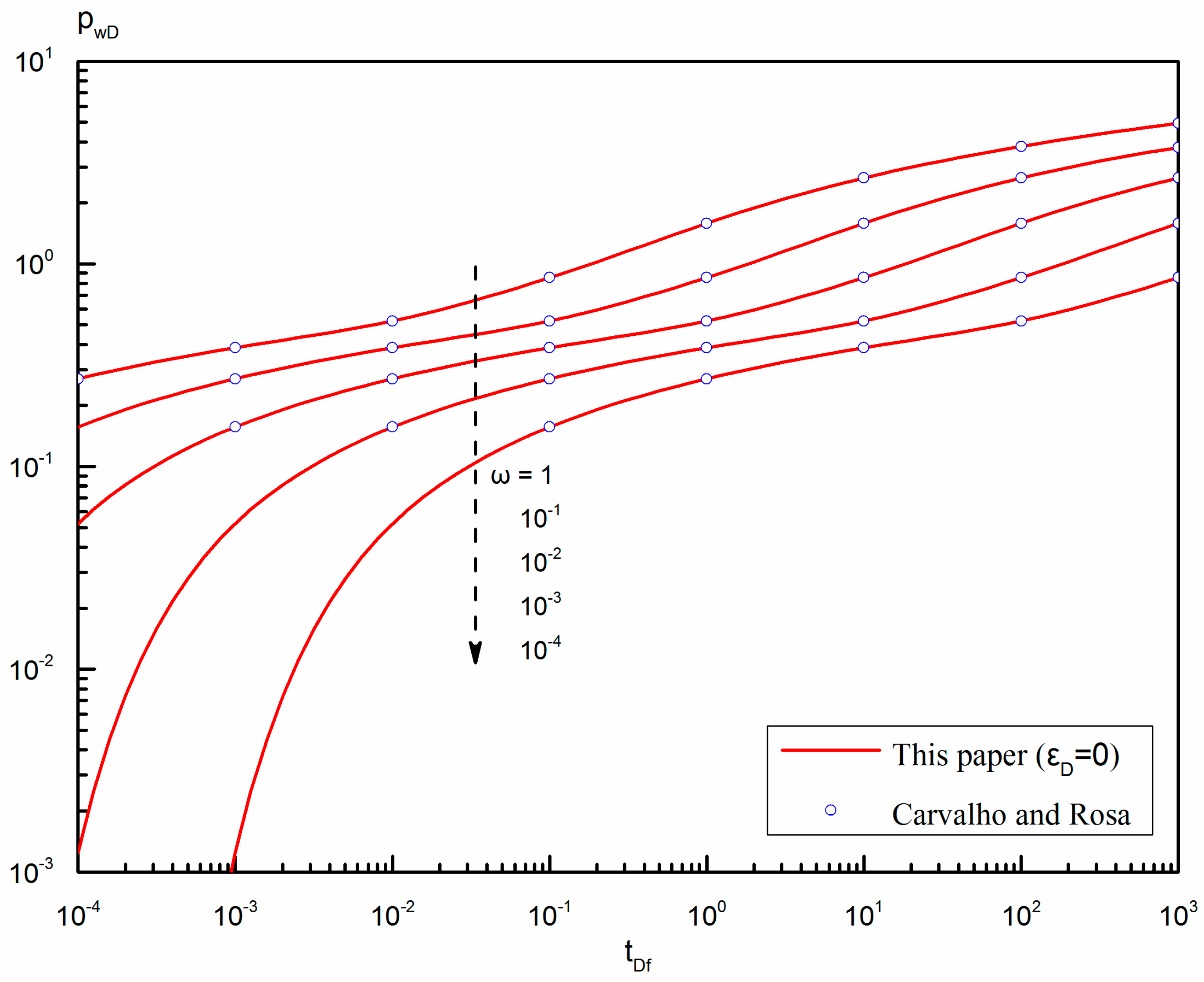
de Carvalho and Rosa [3] presented an infinite-conductivity solution for a horizontal well in the naturally fractured reservoir, but did not consider the effect of the geomechanics, which just corresponds to ${\epsilon }_D=0$ in our model. Note that their pressure was calculated at a fixed point along the wellbore, $x_D=0.68$, by using the uniform-flux solution. They presented a series of type curves for a horizontal well in a dual-porosity reservoir. Thus, we can let $x_D=0.68$ in our uniform-flux solution, Equation (90), to verify our uniform-flux solution.

Due to the difference of the reference length in dimensionless variables between two models, a reasonable transformation of the parameters value should be conducted before the verification. Base on the data presented in the work of de Carvalho and Rosa [3], the parameter values used for the verification are listed in

Table 2. Basic data used for verification of the model.

Parameters in this Work	Values	Parameters in Figure 5 of SPE 18302 [3]	Values
$\omega$	100~10−4	${\omega }^{\ast }$	100~10−4
$\lambda$	10−9	${\lambda }^{\ast }$	10−3
$r_{eD}$	100,000	$r_{eD}{}^{\ast }$	infinite
$h_D$	200	$h_D{}^{\ast }$	0.2
$x_D$	0.68	$x_D{}^{\ast }$	0.68
$y_D$	0.001	$y_D{}^{\ast }$	0.001
$r_{wD}$	0.001	$r_{wD}{}^{\ast }$	0.001
$z_{wD}$	0.5	$z_{wD}{}^{\ast }$	0.5
$C_D$	0	$C_D{}^{\ast }$	0
$S$	0	$S^{\ast }$	0
$L_D$	5
${\epsilon }_D$	0

. Meanwhile, the reservoir boundary in their model is assumed infinite, which is different from our outer boundary. Therefore, we can only select the result in the early time ($t_D\le {10}^3$) to verify our solution. As shown in Figure 3, there is an excellent agreement on pressure response at $x_D=0.68$ between our result and the work of de Carvalho and Rosa [3] for different parameters value. It is also verified that the method in this work can calculate accurately.

6.2. Effect of Dimensionless Elasticity Parameter on Horizontal Wellbore Pressure-Drop Profiles

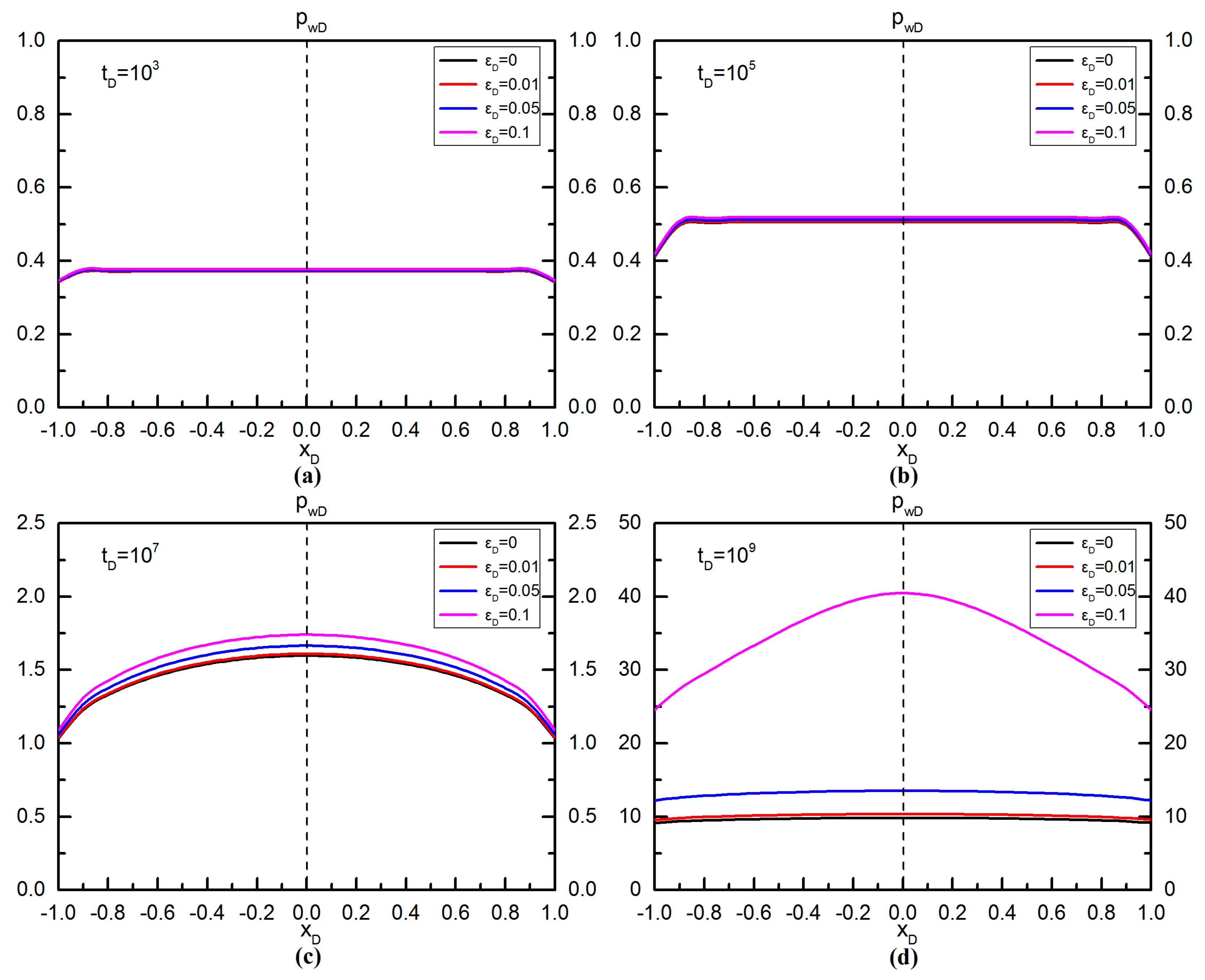
For the uniform-flux case, pressure drop is not uniform along the wellbore face. By using the data in

Table 3. Basic data used in Figure 4.

Parameters	Values	Parameters	Values
$\omega$	0.1	$r_{wD}$	0.00025
$\lambda$	0.003	$z_{wD}$	0.5
$r_{eD}$	4	$L_D$	16
$h_D$	250	$C_D$	0.5
$x_D$	−1~1	$S$	0.25
$y_D$	0	${\epsilon }_D$	0, 0.01, 0.05, 0.1

, Figure 4 discusses the effect of dimensionless elasticity parameter on the wellbore pressure-drop profiles at different time.

Figure 4a,b present the pressure drop profiles with respect to horizontal wellbore position $x_D$ from −1 to 1 for different ${\epsilon }_D$ at $t_D={10}^3,{10}^5$, respectively. We can find that the curves for different ${\epsilon }_D$ almost overlap together in each figure, which means the effect of stress sensitivity is very weak and can be neglected at small time. Meanwhile, the pressure drop profiles in Figure 4a,b are close to a horizontal line and only the pressure drop at both ends of the wellbore is slightly lower than that at the rest of the wellbore. It demonstrates that the ends of the wellbore cause a lower pressure drop under the uniform-flux condition. Figure 4c shows the horizontal wellbore’s pressure-drop profiles at $t_D={10}^7$. It can be seen from Figure 4c that when the dimensionless production time increases to 10⁷, the pressure drop at the same wellbore position $x_D$ slightly increases with the increase of ${\epsilon }_D$, so a stronger stress sensitivity will lead to a larger pressure drop at this time. All the $p_{wD}-x_D$ curves in Figure 4c are symmetric around the vertical line, $x_D=0$, and form a bow shape, and a farther position away from the center of the wellbore corresponds to a lower pressure drop. Figure 4d presents the pressure drop profiles for different ${\epsilon }_D$ at $t_D={10}^9$. Like the profiles in Figure 4c, the $p_{wD}-x_D$ curve for ${\epsilon }_D=0.1$ in Figure 4d also looks like a bow. The $p_{wD}-x_D$ curves for ${\epsilon }_D$ = 0, 0.01 and 0.05 should also be like a bow, but their shapes are not very obvious due to a large scale of $p_{wD}$. Compared with Figure 4c, as ${\epsilon }_D$ increases, the pressure drop at the same wellbore position $x_D$ increases more obviously at this time. Overall, we can conclude that the effect of dimensionless elasticity parameter on the pressure-drop profiles becomes stronger with the stress sensitivity increasing and the production going on, for the reason of a larger fracture permeability reduction from the closure of natural fractures.

6.3. Comparison with a Model Not Considering Geomechanics

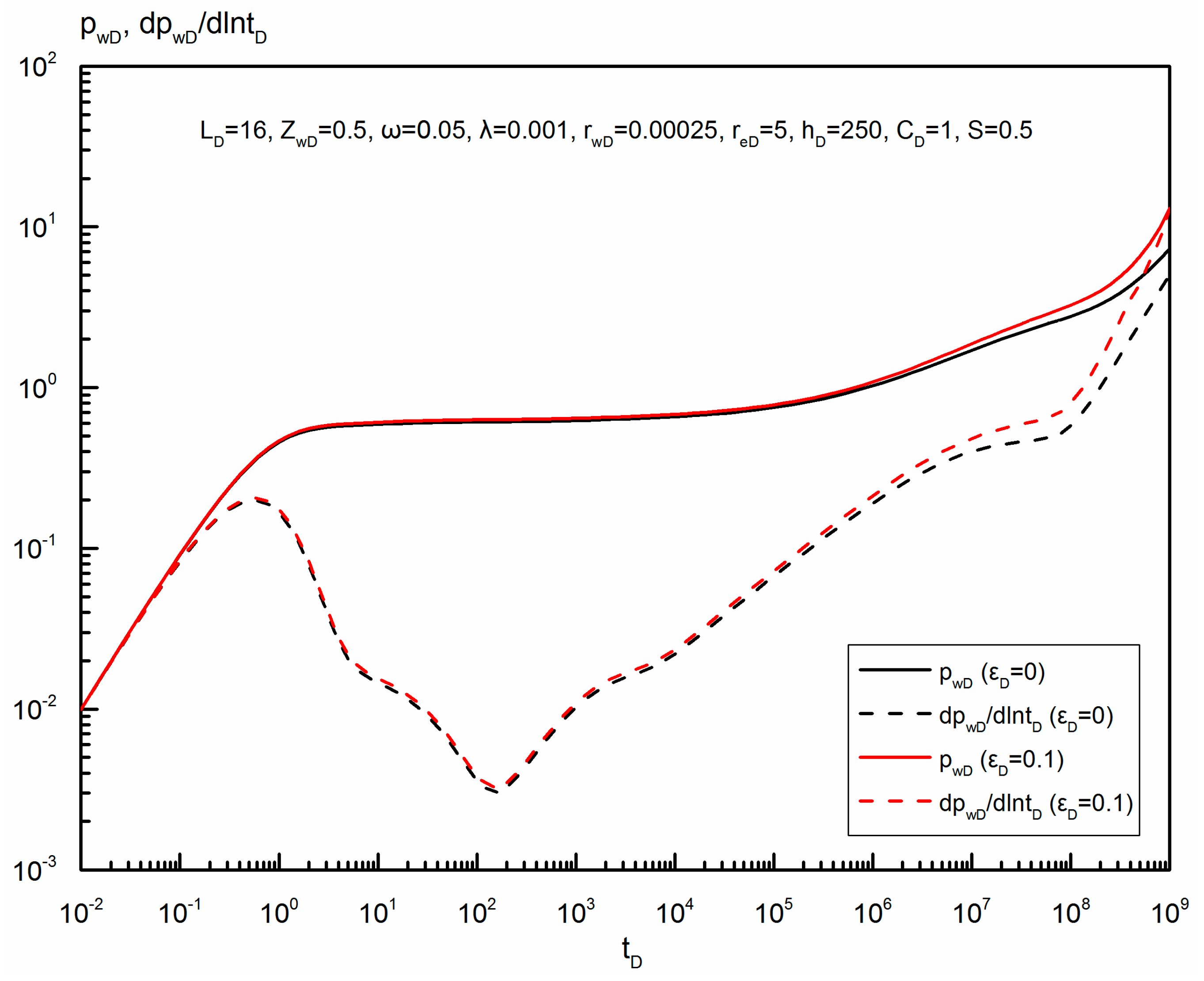
Since we have established a model of a horizontal well incorporating geomechanics, it is necessary to make a comparison with a model not considering geomechanics. In this study, let ${\epsilon }_D$ equal to 0.1 and 0, which represent the model incorporating and not incorporating geomechanics, respectively. Based on the infinite-conductivity solutions, Equation (89) and (91), Figure 5 presents the comparison result of the wellbore pressure and pressure derivative curves of these two models.

As shown in Figure 5, in the early- and middle-flow periods ($t_D\le {10}^{-1}$), the transient pressure almost overlap together, and the pressure derivative curves almost overlap together, too. As the production time gets longer, especially in the late-flow period, the pressure drop of the model incorporating geomechanics becomes larger than that not incorporating geomechanics, so does the pressure derivative. It can be interpreted by that for the model incorporating geomechanics, the closure of natural fractures gets more and more serious, and more reservoir energy will be consumed to produce the same amount of oil.

6.4. Flow Regime Recognition on Transient Wellbore Pressure Curves

The identification of flow regimes is one of the most important procedures of transient pressure analysis. Similarly, we use the infinite-conductivity solution to analyze this case’s flow regimes. Figure 6 shows the transient pressure and pressure derivative responses of a horizontal well incorporating geomechanics in a naturally fractured reservoir (${\epsilon }_D$ = 0.05) and nine typical flow regimes can be observed in Figure 6:

(1)

Pure wellbore storage regime. At small dimensionless time, flow is mainly governed by the wellbore storage effect, and the transient pressure and pressure derivative curves align in an upward straight line with a unit slope.

(2)

First transition flow. This regime is marked by a hump on the pressure derivative curve.

(3)

Radial flow in the natural fracture system. A short radial flow may occur after a transition flow if the reserve ratio in the natural fracture system is large enough. As presented in Figure 6, the pressure derivative curve in this regime is a horizontal line with a value of “$1/\left(4L_D\right)$” and the corresponding streamline distribution in the reservoir is shown in Figure 7a.

(4)

Inter-porosity flow. This regime represents the cross flow from matrix system to natural fracture system. The pressure derivative curve in this regime shows a concave-shaped segment, which is the main characteristic of naturally fractured reservoirs.

(5)

Radial flow in the compound system. When the inter-porosity flow finishes, fluid flow in two systems reaches a dynamic balance, and a second radial flow begins to occur in the compound system. A horizontal line with a value of “$1/\left(4L_D\right)$” can be also observed on the pressure derivative curve in this regime and its streamline distribution is the same with that in the third flow regime (as shown in Figure 7a).

(6)

Linear flow in the compound system. In this regime, the dominating flow is linear flow in the horizontal plane, and the streamlines are parallel to the upper and lower boundary (as shown in Figure 7b). Its pressure derivative curve shows an upward straight line with a half slope.

(7)

Second transition flow. As the drainage area expands, a second transition flow may occur in the reservoir before it reaches a pseudo-radial flow in the horizontal plane.

(8)

Pseudo-radial flow in the compound system. When reservoir radius is large enough, a pseudo-radial flow in the horizontal plane may be formed after the second transition flow (as shown in Figure 7c). Unlike the conventional reservoir, due to the effect of stress sensitivity, the pressure derivative curve is not a horizontal line with a value of “0.5” but exhibits an upward tendency.

(9)

Pseudo-steady flow in the compound system. When the transient wave reaches the outer boundary, both the transient pressure curve and pressure derivative curves go up rapidly, and their slopes are greater than “1” due to stress sensitivity (as shown in Figure 6).

6.5. Analysis of Parameters’ Influence on Transient Pressure Behavior

In this section, we investigated several important parameters’ influence on the transient response of the proposed model in this work. Note that these investigations are based on the infinite-conductivity solution proposed in this work. The influence of wellbore storage coefficient, skin factor, interporosity flow coefficient and fracture storage capacity, has been discussed in the literature, and will not be further discussed here.

6.5.1. Dimensionless Elasticity Parameter

Figure 8 shows the influence of dimensionless elasticity parameter ${\epsilon }_D$ on the transient response. Its influence is mainly concentrated in the late-flow period. For the case not incorporating geomechanics (${\epsilon }_D=0$), the pressure derivative curve is a horizontal line with a value of 0.5 in the pseudo-radial regime, and is an upward straight line with a unit slope in the pseudo-steady flow regime. However, when the geomechanics is incorporated, the pressure derivative curve bends upward in the late-flow period. It can be concluded that with the increase of ${\epsilon }_D$, the slope of the derivative curve in the late-flow period becomes larger, which means a greater pressure drop.

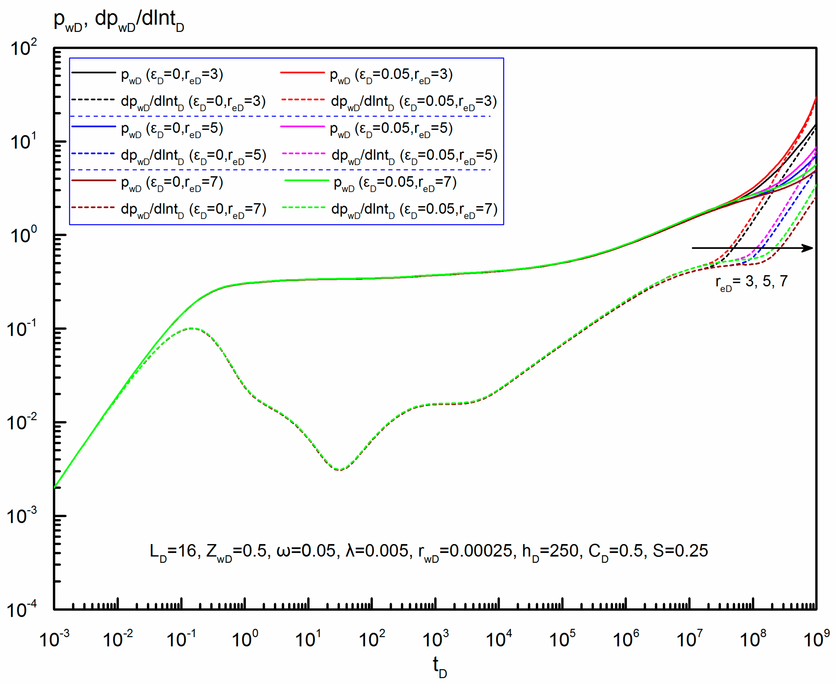
6.5.2. Dimensionless Reservoir Radius

Figure 9 presents the effect of dimensionless reservoir radius $r_{eD}$ on the transient pressure behavior. Due to the closed boundary, this parameter also mainly influences the oil flow in the late-flow period, and a smaller dimensionless reservoir radius will cause the final pseudo-steady flow to occur earlier. We also can see in Figure 9 that in the pseudo-steady flow regime, at the same production time, in terms of the pressure and pressure derivative, their differences between the models incorporating and not incorporating geomechanics, are increasing significantly with the decrease of dimensionless reservoir radius. It can be interpreted by that, with the production going on, the continuous fracture closure is more serious for the reservoir with a smaller dimensionless reservoir radius, and the effect of stress sensitivity on the transient response becomes stronger, too.

6.5.3. Dimensionless Reservoir Thickness

Figure 10 demonstrates the effect of dimensionless reservoir thickness $h_D$ on transient pressure dynamics of a horizontal well in the naturally fractured reservoir. Obviously, it has a great influence on the early-flow period, including the following regimes: first transition flow, radial flow in the natural fracture system, inter-porosity flow and radial flow in the compound system, but has no influence on the middle- and late-flow periods. There is an implicit relationship between dimensionless wellbore radius, wellbore length and reservoir thickness, $r_{wD}{L}_D{h}_D=1$. In this study, let $h_D$ equal to 200, 250 and 400, and the corresponding $L_D$ is 300, 400 and 500, respectively. As shown in Figure 10, the concave-shaped segment gradually uplifts with the increase of dimensionless reservoir thickness and the value of the pressure derivative in two radial flow regimes is 1/80, 1/64 and 1/40, respectively. However, the change of dimensionless reservoir thickness does not enhance or weaken the effect of stress sensitivity like dimensionless radius reservoir and its effect will not extend to the late-flow period.

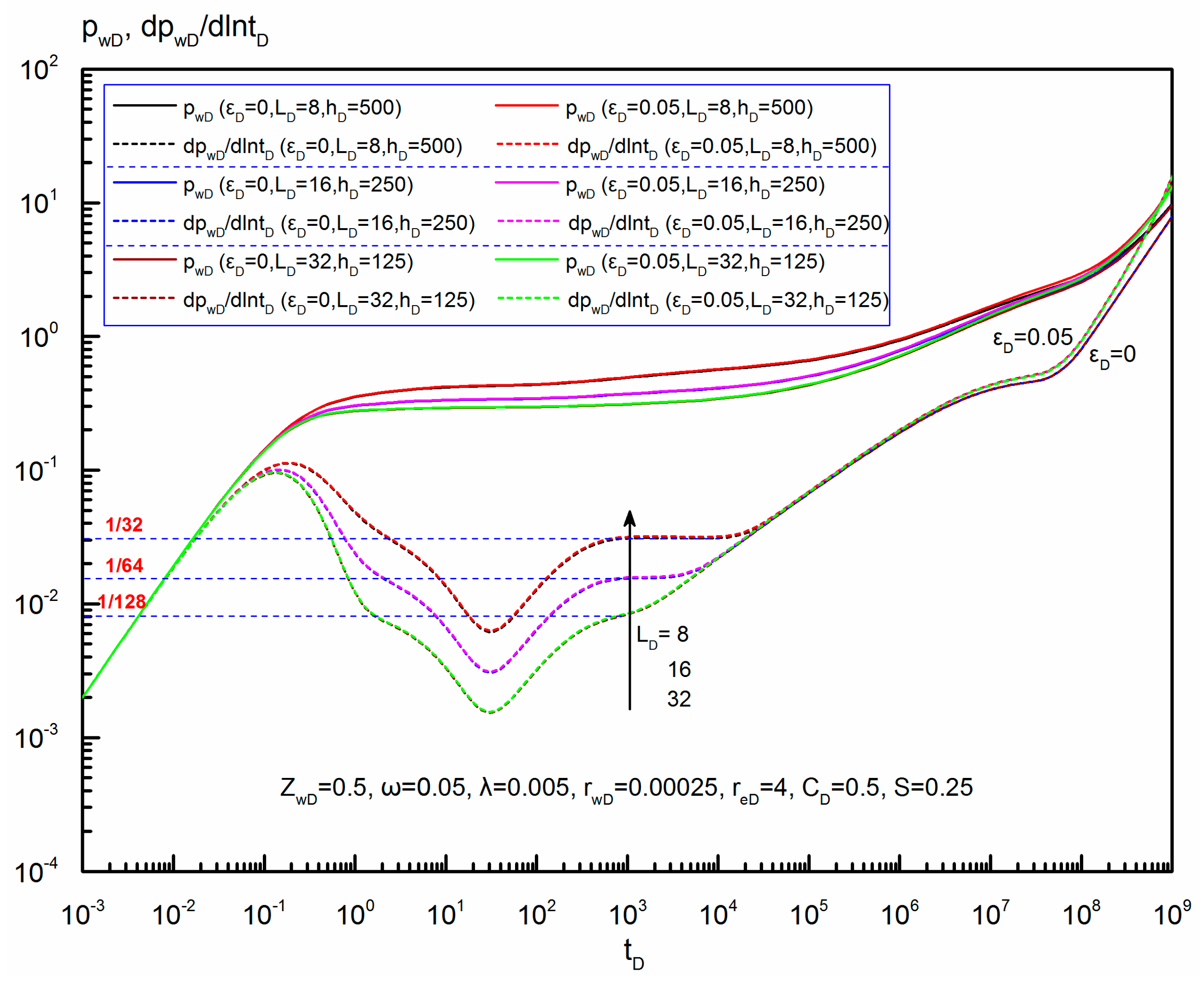
6.5.4. Dimensionless Horizontal Wellbore Length

Figure 11 shows the effect of dimensionless horizontal wellbore length $L_D$ on transient pressure behavior. As presented in Figure 11, the influence of dimensionless wellbore length is similar to that of dimensionless reservoir thickness on the transient pressure behavior and this parameter also mainly affects the early-flow period. Their differences lie in that the concave-shaped segment gradually descents with the increase of dimensionless wellbore length.

6.5.5. Dimensionless Wellbore Vertical Position

Figure 12 shows the effect of dimensionless wellbore vertical position $z_{wD}$ on transient response. This parameter only influences the duration and occurrence of radial flow in the compound system. Similarly, the change of wellbore vertical position will not enhance or weaken the effect of stress sensitivity and its impact does not extend to the late-flow period.

6.6. Analysis of the Influence of Geomechanical Parameters in North Truva Field

Here we take KT-I formation of North Truva field in Kazakhstan, a typical fractured formation, as an example to understand the influence of geomechanical parameters on the elasticity parameter and transient response. Note that the elasticity parameter $\epsilon$ is dimensional and its unit is Pa⁻¹.

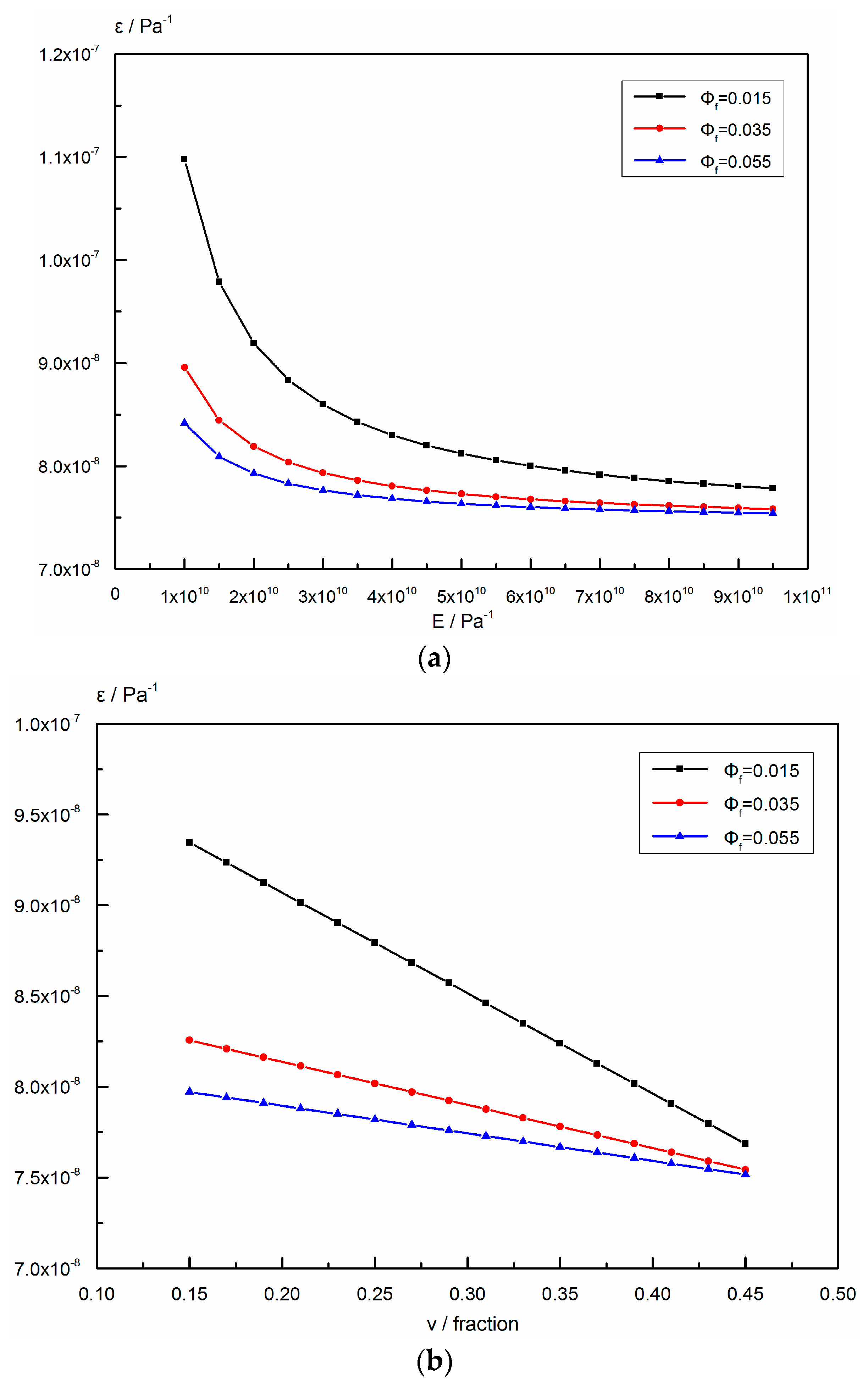
6.6.1. Influence of Geomechanical Parameters on the Elasticity Parameter

Considering the data of KT-I formation presented in

Table 4. Basic data of KT-I formation in North Truva field.

Formation Parameters	Values
Poisson’s ratio	0.15–0.45
Young’s modulus	1.0 × 1010–9.5 × 109 Pa
Fracture porosity	0.015–0.055
Fracture compressibility	2.39 × 10−8 Pa−1
Oil compressibility	2.26 × 10−9 Pa−1

, we focused on two important geomechanical parameters, Young’s modulus $E$ and Poisson’s ratio $\nu$, to investigate their influence on the elasticity parameter $\epsilon$.

According to the definition of elasticity parameter $\epsilon$ in Equation (28), we calculate the valve of elasticity parameter for different Young’s modulus at ${\varphi }_f$ = 0.015, 0.035 and 0.055 respectively, and then plot the curves of $\epsilon -E$ (as shown in Figure 13a). It can be observed that for a given fracture porosity, as the Young’s modulus of reservoir rock increases, the elasticity parameter first decreases sharply, and then decreases slowly, and finally decreases very slowly and even this slight decrease can be neglected. Similarly, we plot the curves of $\epsilon -\nu$ at ${\varphi }_f$ = 0.015, 0.035 and 0.055 (as shown in Figure 13b). We can see that the elasticity parameter linearly decreases with the increase of Poisson’s ratio at a given fracture porosity. Combining Figure 13a with Figure 13b, it can be concluded that under the same values of Young’s modulus and Poisson’s ratio, the elasticity parameter will decrease with the increase of fracture porosity. Using the properties of KT-I formation, its elasticity parameter $\epsilon$ ranges from $8\times {10}^{-8}$ Pa⁻¹ to $1.1\times {10}^{-7}$ Pa⁻¹.

6.6.2. Influence of Geomechanical Parameters on the Transient Response of H519

We select a horizontal well in KT-I formation, H519, to observe the influence of Young’s modulus and Poisson’s ratio on this horizontal well’s transient pressure behavior. The reservoir and fluid parameters used to calculate the transient pressure are presented in Figure 14 and Figure 15, respectively.

As demonstrated in Figure 14, for H519 in North Truva field, when Young’s modulus increases from $1.0\times {10}^{-10}$ Pa⁻¹ to $4.0\times {10}^{-10}$ Pa⁻¹, and then to $7.0\times {10}^{-10}$ Pa⁻¹, the early- and middle-time transient responses of this horizontal well are almost the same, but a slight difference between them occurs in the late-time flow period. Through the enlarged image of the late-time curves, we can see that both the transient pressure and pressure derivative in the pseudo-steady flow regime decrease with the increase of Young’s modulus. Similarly, from Figure 15, the early- and middle-time transient response is also not affected by the change of Poisson’s ratio, and when Poisson’s ratio varies from 0.15 to 0.45, the transient pressure and pressure derivative in the late-time flow period gradually decrease. Overall, the transient response of H519 has a slight negative correlation with Young’s modulus and Poisson’s ratio in the late-time flow period, especially in the pseudo-steady flow regime.

7. Conclusions

This paper presents a new model of a horizontal well incorporating geomechanics in the naturally fractured reservoir. The analytical pressure solutions for the uniform-flux and infinite-conductivity horizontal wells including Young’s modulus and Poisson’s ratio are derived by using Pedrosa transform, perturbation technique and spatial integral method. Based on this study, several important conclusions are obtained:

(1)

For a uniform-flux horizontal well, the effect of dimensionless elasticity parameter on the pressure drop profiles becomes stronger as the production time gets longer, due to a larger fracture permeability reduction caused by the closure of natural fractures. When the effect of dimensionless elasticity parameter is strong enough, the profile looks like a bow, and a farther position away from the center of the horizontal wellbore corresponds to a lower pressure drop.

(2)

For an infinite-conductivity horizontal well, while the production going on, especially in the late-flow period, the pressure drop of the model incorporating geomechanics becomes larger than that not incorporating geomechanics, and more reservoir energy will be consumed to produce the same amount of oil.

(3)

Nine typical flow regimes can be observed on the transient response of the infinite-conductivity horizontal well incorporating geomechanics. The differences between the models incorporating and not incorporating this property lie in the final flow regimes. Due to the stress sensitivity, the pressure derivative curve is not a horizontal line with a value of “0.5” but exhibits an upward tendency in the pseudo-radial flow in the compound system, and in the pseudo-steady flow regime, both the transient pressure curve and the pressure derivative curve rise quickly and their slope is greater than “1”.

(4)

Analysis of parameters’ influence on the transient pressure behavior shows that dimensionless elasticity parameter and dimensionless reservoir radius mainly affect the late-flow period, but dimensionless reservoir thickness, dimensionless wellbore length and dimensionless wellbore vertical position mainly influence the early-flow period. There is a larger pressure drop with the increase of dimensionless elasticity parameter or the decrease of dimensionless reservoir radius in the late-flow period.

(5)

For the KT-I formation of the North Truva field, the elasticity parameter decreases with the increase of Young’s modulus or Poisson’s ratio at a given fracture porosity and this parameter ranges from $8\times {10}^{-8}$ Pa⁻¹ to $1.1\times {10}^{-7}$ Pa⁻¹ in this formation. Calculation results show that the transient response of H519 has a slight negative correlation with Young’s modulus and Poisson’s ratio in the late-flow period, especially in the pseudo-steady flow regime.

References

- Ozkan, E.; Raghavan, R.; Joshi, S.D. Horizontal well pressure analysis. In Proceedings of the SPE California Regional Meeting, Ventura, CA, USA, 8–10 April 1987. Paper No. 16378. [Google Scholar] [CrossRef]
- Ozkan, E. Performance of Horizontal Wells. Ph.D. Thesis, Tulsa University, Tulsa, OK, USA, 1988. [Google Scholar]
- De Carvalho, R.S.; Rosa, A.J. Transient pressure behavior for horizontal wells in naturally fractured reservoir. In Proceedings of the SPE Annual Technical Conference and Exhibition, Houston, TX, USA, 2–5 October 1988. Paper No. 18302. [Google Scholar] [CrossRef]
- Rosa, A.J.; de Carvalho, R.S. A mathematical model for pressure evaluation in an lnfinite-conductivity horizontal well. SPE Form. Eval. 1989, 4, 559–566. [Google Scholar] [CrossRef]
- Jones, F.O.; Owens, W.W. A laboratory study of low-permeability gas sands. J. Pet. Technol. 1980, 32, 1631–1640. [Google Scholar] [CrossRef]
- Economides, M.J.; Buchsteiner, H.; Warpinski, N.R. Step-pressure test for stresssensitive permeability determination. In Proceedings of the SPE Formation Damage Control Symposium, Lafayette, LA, USA, 7–10 February 1994. Paper No. 27380. [Google Scholar]
- Farquhar, R.A.; Smart, B.G.D.; Todd, A.C.; Tompkins, D.E.; Tweedie, A.J. Stress sensitivity of lowpermeability sandstones from the rotliegendes sandstone. In Proceedings of the SPE Annual Technical Conference and Exhibition, Houston, TX, USA, 3–6 October 1993. Paper No. 26501. [Google Scholar] [CrossRef]
- Xu, W.; Wang, X.; Hou, X.; Clive, K.; Zhou, Y. Transient analysis for fractured gas wells by modified pseudo-functions in stress-sensitive reservoirs. J. Nat. Gas Sci. Eng. 2016, 35, 1129–1138. [Google Scholar] [CrossRef] [Green Version]
- Wang, H.; Guo, J.; Zhang, L. A semi-analytical model for multilateral horizontal wells in low-permeability naturally fractured reservoirs. J. Petrol. Sci. Eng. 2017, 149, 564–578. [Google Scholar] [CrossRef]
- Barenblatt, G.I.; Zheltov, Y.P. Fundamental equations for the flow of homogeneous fluids through fissured rocks. Dokl. Akad. Nauk SSSK 1960, 132, 545–548. [Google Scholar]
- Barenblatt, G.I.; Zheltov, Y.P.; Kochina, I.N. Basic concepts in the theory of seepage of homogeneous liquids in fissured rocks. J. Appl. Math. Mech. 1960, 24, 1286–1303. [Google Scholar] [CrossRef]
- Nelson, R. Geologic Analysis of Naturally Fractured Reservoirs; Gulf Professional Publishing: Houston, TX, USA, 1985. [Google Scholar]
- Vasilev, I.; Alekshakhin, Y.; Kuropatkin, G. Pressure transient behavior in naturally fractured reservoirs: Flow anaysis. In Proceedings of the SPE Annual Caspian Technical Conference & Exhibition, Astana, Kazakhstan, 1–3 November 2016. Paper No. 182562. [Google Scholar] [CrossRef]
- Warren, J.E.; Root, P.J. The behavior of naturally fractured reservoirs. SPE J. 1963, 3, 245–255. [Google Scholar] [CrossRef]
- Kazemi, H. Pressure transient analysis of naturally fractured reservoirs with uniform fracture distribution. SPE J. 1969, 9, 451–462. [Google Scholar] [CrossRef]
- De Swaan, O.A. Analytic solutions for determining naturally fractured reservoir properties by well testing. SPE J. 1976, 16, 117–122. [Google Scholar] [CrossRef]
- Nur, A.; Yilmaz, O. Pore Pressure in Fronts in Fractured Rock Systems; Department of Geophysics, Stanford University: Stanford, CA, USA, 1985. [Google Scholar]
- Kikani, J.; Pedrosa, O.A. Perturbation analysis of stress-sensitive reservoirs. SPE Form. Eval. 1991, 6, 379–386. [Google Scholar] [CrossRef]
- Chen, M.; Bai, M. Modeling stress-dependent permeability for anisotropic fractured porous rocks. Int. J. Rock Mech. Min. 1998, 35, 1113–1119. [Google Scholar] [CrossRef]
- Raghavan, R.; Chin, L.Y. Productivity changes in reservoirs with stress-dependent permeability. In Proceedings of the SPE Annual Technical Conference and Exhibition, San Antonio, TX, USA, 29 September–2 October 2002. Paper No. 77535. [Google Scholar] [CrossRef]
- Oluyemi, G.F.; Ola, O. Mathematical modelling of the effects of in-situ stress regime on fracture-matrix flow partitioning in fractured reservoirs. In Proceedings of the Nigeria Annual International Conference and Exhibition, Tinapa, Calabar, Nigeria, 31 July–7 August 2010. Paper No. 136975. [Google Scholar] [CrossRef]
- Jabbari, H.; Zeng, Z.; Ostadhassan, M. Impact of in-situ stress change on fracture conductivity in naturally fractured reservoirs: Bakken case study. In Proceedings of the 45th U.S. Rock Mechanics/Geomechanics Symposium, San Francisco, CA, USA, 26–29 June 2011. Paper No. ARMA-11-239. [Google Scholar]
- Celis, V.; Silva, R.; Ramones, M.; Guerra, J.; Da Prat, G. A new model for pressure transient analysis in stress sensitive naturally fractured reservoirs. SPE Adv. Technol. Ser. 1994, 2, 126–135. [Google Scholar] [CrossRef]
- Samaniego, V.F.; Villalobos, L.H. Transient pressure analysis of pressure dependent naturally fractured reservoirs. J. Petrol. Sci. Eng. 2003, 39, 45–56. [Google Scholar] [CrossRef]
- Yao, S.; Zeng, F.; Liu, H. A semi-analytical model for hydraulically fractured wells with stress-sensitive conductivities. In Proceedings of the SPE Unconventional Resources Conference Canada, Calgary, AB, Canada, 5–7 November 2013. Paper No. 167230. [Google Scholar] [CrossRef]
- Zhang, Z.; He, S.; Liu, G.; Guo, X.; Mo, S. Pressure buildup behavior of vertically fracturedwells with stress-sensitive conductivity. J. Petrol. Sci. Eng. 2014, 122, 48–55. [Google Scholar] [CrossRef]
- Rosalind, A. Impact of stress sensitive permeability on production data analysis. In Proceedings of the SPE Unconventional Reservoirs Conference, Keystone, CO, USA, 10–12 February 2008. Paper No. 114166. [Google Scholar] [CrossRef]
- Robertson, E.P.; Christiansen, R.L. A permeability model for coal and other fractured, sorptive-elastic media. In Proceedings of the SPE Eastern Regional Meeting, Canton, OH, USA, 11–13 October 2006. Paper No. 104380. [Google Scholar] [CrossRef]
- Janna, W.S. Introduction to Fluid Mechanics; CRC Press: Boca Raton, FL, USA, 2009. [Google Scholar]
- Zhang, J.; Bai, M.; Roegiers, J.C.; Liu, T. Determining stress-dependent permeability in the laboratory. In Proceedings of the 37th U.S. Symposium on Rock Mechanics, Vail, CO, USA, 7–9 June 1999; Volume 37, pp. 341–347. [Google Scholar]
- McKee, C.R.; Bumb, A.C.; Koenig, R.A. Stress-dependent permeability and porosity of coal and other geologic formations. SPE Form. Eval. 1988, 3, 81–91. [Google Scholar] [CrossRef]
- Pedrosa, O.A. Pressure transient response in stress-sensitive formations. In Proceedings of the SPE California Regional Meeting, Oakland, CA, USA, 2–4 April 1986. Paper No. 15115. [Google Scholar] [CrossRef]
- He, J.H. Homotopy perturbation technique. Comput. Methods Appl. Mech. Eng. 1999, 178, 257–262. [Google Scholar] [CrossRef]
- He, J.H. A coupling method of a homotopy technique and a perturbation technique for non-linear problems. Int. J. Non-Linear Mech. 2000, 35, 37–43. [Google Scholar] [CrossRef]
- Gringarten, A.C.; Ramey, H.J., Jr. The use of source and Green’s functions in solving unsteady-flow problems in reservoirs. SPE J. 1973, 13, 285–296. [Google Scholar] [CrossRef]
- Gringarten, A.C.; Ramey, H.J., Jr.; Raghavan, R. Unsteady-state pressure distributions created by a well with a single infinite-conductivity vertical fracture. SPE J. 1974, 14, 347–360. [Google Scholar] [CrossRef]
- Clonts, M.D.; Ramey, H.J., Jr. Pressure-transient analysis for wells with horizontal drainholes. In Proceedings of the SPE California Regional Meeting, Oakland, CA, USA, 2–4 April 1986. Paper No. 15116. [Google Scholar] [CrossRef]
- Daviau, F.; Mouronval, G.; Bourdarot, G.; Curutchet, P. Pressure analysis for horizontal wells. SPE Form. Eval. 1988, 3, 716–724. [Google Scholar] [CrossRef]
- Kuchuk, F.J.; Goode, P.A.; Wilkinson, D.J.; Thambynayagam, R.K.M. Pressure-transient behavior of horizontal wells with and without gas cap or aquifer. SPE Form. Eval. 1991, 6, 86–94. [Google Scholar] [CrossRef]
- Van Everdingen, A.F. The skin effect and its influence on the productive capacity of a well. J. Pet. Technol. 1953, 5, 171–176. [Google Scholar] [CrossRef]
- Kucuk, F.; Ayestaran, L. Analysis of simultaneously measured pressure and sandface flow rate in transient well testing. J. Pet. Technol. 1985, 37, 323–334. [Google Scholar] [CrossRef]
- Stehfest, H. Algorithm 368: Numerical inversion of Laplace transforms. Commun. ACM 1970, 13, 47–49. [Google Scholar] [CrossRef]
Figure 1.
Horizontal well model in the closed cylindrical system.
Figure 2.
Fracture porosity definition in a naturally fractured reservoir.
Figure 3.
Verification of a horizontal well in a naturally fractured reservoir without stress sensitivity ().