Collaborative Optimization of Post-Disaster Damage Repair and Power System Operation

The Shaanxi Key Laboratory of Smart Grid, The State Key Laboratory of Electrical Insulation and Power Equipment, Xi’an Jiaotong University, Xi’an 710049, China
*
Author to whom correspondence should be addressed.
Energies 2018, 11(10), 2611; https://doi.org/10.3390/en11102611
Submission received: 8 August 2018
/
Revised: 26 August 2018
/
Accepted: 28 August 2018
/
Published: 30 September 2018
(This article belongs to the Section F: Electrical Engineering)
Abstract
:After disasters, enhancing the resilience of power systems and restoring power systems rapidly can effectively reduce the economy damage and bad social impacts. Reasonable post-disaster restoration strategies are the most critical part of power system restoration work. This paper co-optimizes post-disaster damage repair and power system operation together to formulate the optimal repair route, the unit output and transmission switching plan. The power outage loss will be minimized, with possible small expense of damage repair and power system operation cost. The co-optimization model is formulated as a mixed integer second order cone program (MISOCP), while the AC-power-flow model, the complex power system restoration constraints and the changing processes of component available states are synthetically considered to make the model more realistic. Lagrange relaxation (LR) decomposes the model into the damage repair routing sub problem and the power system operation sub problem, which can be solved iteratively. An acceleration strategy is used to improve the solving efficiency. The proposed model and algorithm are validated by the IEEE 57-bus test system and the results indicate that the proposed model can realize the enhancement of resilience and the economic restoration of post-disaster power systems.
1. Introduction
Power systems have become an indispensable guarantee for the prosperity and development of modern society. Traditionally, power systems are designed to be reliable enough under normal conditions and to sustain single outage contingency (“N−1” security criterion). However, on one hand, due to the current climate change, power systems are more likely to suffer disturbances from extreme natural disasters, which possibly lead to cascading outages and blackouts. In 2008, a severe ice storm hit southern China [1], resulting in the failure of 7541 lines; in 2011, more than 4 million household power supply was affected by Japan’s earthquake [2]. These disasters include earthquake, strong wind, ice storm, lightning, extreme temperature, rainstorm and flood and so forth. On the other hand, increasing man-made and terrorist attacks have also greatly harmed the safe and stable operation of power systems. In 2013, the PG&E substation in Metcalf of California was shot, causing the breakdowns of 17 transformers and a serious power outage [3]. To make power systems stronger and smarter to resist disasters, the concept of resilience of power systems which has aroused extensive attention is proposed.
According to [4], power system resilience is “the ability of the power system to anticipate high-impact low-probability events, rapidly recover from these disruptive contingencies and absorb lessons for adapting its operation and structure for preventing or mitigating the impact of similar events in future.” According to the evolving nature of general disasters, reference [5] divided the research of power system resilience into three parts: pre-disaster system toughness, during-disaster system resistance and post-disaster system restoration ability, as shown in Figure 1. As the core part of resilience research, the enhancement strategies of resilience can also be implemented from the three aspects. Pre-disaster improvement mainly belongs to the scope of hardening measures, while during-disaster and post-disaster improvement are dominated by smart operational measures. Before the occurrence of disasters, it is essentially to optimize power system resilience-oriented planning [6,7,8], identify and strengthen the weak links [9,10], as well as allocate the disaster repair resources optimally [11,12]. During disasters, effective and flexible control measures [13,14] should be taken to avoid cascading failures and restrict the further expansion of failures. After disasters, how to rapidly repair the damaged components and restore curtailed load with limited resources [15,16,17] is the most urgent and significant task for power system restoration. In [18], an analysis of lifelines in case of seismic disaster under the analysis FMECA was presented. Reference [19] reviewed the challenges of maintaining the linear assets and provided a conceptual framework for the use of autonomous inspection and maintenance practices. This paper emphasizes the enhancement of resilience in the post-disaster stage.
In the previous power system post-disaster resilience improvement studies, concentrations are focused more on the restoration after large-scale blackouts, while the researches are primarily carried out from three aspects: black-start [20,21,22], network reconfiguration [23,24,25] and load restoration [26,27]. However, the interconnection of regional large power systems, reasonable protection and automatic devices, along with advanced alarm processing and fault diagnosis technology, can restrict most electrical faults and accidents in local areas [5]. Therefore, the happening probability of extreme weather events leading to large-scale blackouts is tiny. Compared with the system-wide blackout, local outages are more likely to occur. Nevertheless, the studies on the restoration of local power systems are relatively scarce and immature. Thus, it is more meaningful and practical to study the restoration of local power systems especially considering the repair of damaged components.
Currently, many studies are trying to take the damage repair work into consideration when restoring the post-disaster system. For example, reference [28] discussed the last-mile disaster recovery for power systems, that is, how to schedule and route repair crews to restore the power network as fast as possible. Further work was developed in [29], where a randomized adaptive vehicle decomposition technique was used. However, these methods neglect the coordination of damage repair and power system restoration, which is regarded as a challenging problem [30]. Reference [30] modeled the transportation of repair crews as a vehicle routing problem (VRP) in detail and a two-stage method for the repair and restoration of distribution networks was proposed to minimize the sizes and durations of outages. But the model is for distribution networks and not suitable for the generation and transmission systems. Besides, existing models cannot consider many complex post-disaster system restoration constraints precisely and synthetically or depict the dynamic changing processes of component available states. Ignorance of these constraints may make the obtained restoration scheme infeasible in reality. In addition, the model of power system restoration considering damage repair is a non-convex and non-linear optimization problem, which cannot be solved easily.
Based on the above studies, this paper proposes a novel co-optimization model to coordinate the damage repair work with system operation in post-disaster restoration for generation and transmission system. Once the damage information is available for utilities, the maintenance department can make the best damage repair route. Simultaneously, according to the anticipated available states of fault components, the dispatching department will change the system operation state. Consequently, the economic loss of outage will be minimized, with reasonable repair and system operation cost. The AC-power-flow model, the post-disaster power system restoration complex constraints and the changing processes of component states are involved systematically and integrally, which makes up the shortcomings of existing studies. Moreover, to improve the efficiency of the algorithm, Lagrange relaxation is used to decompose the model into the upper sub problem of routing repair crews and the lower sub problem of power system operation optimization. Further, the acceleration strategy is adopted to speed up the convergence of the MISOCP model. The proposed model is tested on the IEEE 57-bus test system.
The remainder of this paper is organized as follows. Section 2 describes the proposed model. Section 3 presents the mathematical formulation of the model. The LR-based acceleration strategy is discussed in Section 4. Numerical studies are provided in Section 5 to exhibit the effectiveness and application values of the proposed model. Finally, the conclusions are drawn in Section 6.
2. Model Description
The electrical equipment in the power system, especially buses and transmission lines, are often exposed outdoors, accounting for why they are vulnerable to the external disturbances. The damaged components will have adverse effects on the save and stable operation of power systems, leading to the occurrence of generator tripping, load shedding, system splitting or even the breakdown of power systems. Once the disaster strikes, it is critical to route repair crew to repair the damaged components, restore outage load as soon as possible and provide reliable power supply for power users.
In our co-optimization model, we propose a decision-making method for utilities to restore post-disaster power systems. After a disaster, damage assessment will be conducted to acquire the states of components, locate faults and estimate the expected time to repair (TTR) as well as the required resource number of damaged components. Afterwards the best repair scheme is made and repair teams will drive to damaged points and then fix them up based on the optimized task and route. Meanwhile, power system dispatchers will obtain the available states of system equipment and formulate the system operation mode through adjusting the output of units and switching transmission lines. The whole repair-dispatching procedure will maximally reduce the customer interruption cost, while the system operation and repair expense will be minimized.
It is worth noticing that compared to existing models, this research incorporates the second-order-based AC power flow constraints and takes the important constraints during the restoration of power systems into account, which makes the model more accurate and practical to describe the actual restoration process of post-disaster power systems.
After the acquisition of the repair and the system restoration scheme, the anticipated restoration effects can be assessed by the method proposed in [5], which helps to reflect the effectiveness and economic benefits of the strategy and compare the pros and cons of different restoration scenarios.
3. Mathematical Model
The main aim of the model is to restore curtailed load through repairing damaged components, starting up outage units, switching transmission lines and adjusting unit output. During the restoration process, to maintain the stability and improve the control ability of the system, generators are kept in running state. When all the faults are cleared and the power system returns to the normal state, the optimal unit commitment scheme is implemented by adjusting the start-stop status and output of units, in order to realize the economic dispatch, which is beyond the scope of this study.
It is necessary to explain the assumptions first before presenting the model.
- All repair teams are capable of repairing any type of damage. Once a damaged component is repaired, repair team will leave for the next one immediately, until all the tasks are completed.
- The repair time and resource to fix a fault is known and certain; the vehicle speed of repair teams is fixed.
- During the process of damage repair and system restoration, no extra new equipment damage occurs.
- The repair expense of fault points and the outage unit restoration cost are fixed, which have nothing to do with the repair moment or repair teams.
- Generators are not damaged by disasters because they are often located indoors.
3.1. Objective Function
The objective is to minimize the power outage loss, with possible small expense of damage repair and power generation cost, as shown in (1)
where Cope indicates the generation costs of all generators [31], Crep represents the damage repair cost, including labor and transportation cost and Closs is the total economic loss due to outage during the restoration horizon. α1, α2 and α3 are weight factors. As the restoration of lost load is the most urgent mission when there is power outage, the value of α3 is correspondingly larger.
Besides, we need to point out that because the repair cost and unit restoration cost are fixed once the damaged components are identified, they are not involved in the objective function.
3.2. Constraints
3.2.1. Constraints of Damage Repair
- Constraints of damage repair routing
The damage repair routing constraints [28] are displayed in this part, helping to find the optimal routes and tasks for each team. In the repair route of team c, if c leaves damaged component x for y, Mx,y,c equals to 1. Constraint (2) ensures that team c will leave damaged component y once y is repaired. Constraints (3) and (4) ensure that each team starts from the repair center and constraints (5)–(7) ensure that each team finally returns to the repair center after all the missions are completed. If damaged component x is repaired by team c, Nx,c equals 1. Constraint (8) ensures that each damage point will be repaired by one and only one team, avoiding the overlap of tasks. Constraint (9) builds the relationship between Nx,c and Mx,y,c. If team c travels from x to y, then Nx,c equals to 1.
- Constraints of repair resources
Constraints in this part help to reflect the resource abundance and availability, which is an important factor to be considered in the damage repair work. Constraint (10) indicates that the repair resources needed by team c to finish its assignment should not exceed its capacity limit, while constraint (11) ensures that the repair center has enough resources to serve all repair teams.
- Constraints of damaged component states
The time it takes for x to return to the normal state is composed of the waiting time, the route time of repair teams and the repair time. Constraint (12) helps to find the arrival time of team c at fault component y. Team c arrives at x at ATx,c and time RTx,c is spent to repair the damage. Then it takes dx,y time to drive to y. The big M method ensures that the constraint does not work if Mx,y,c is 0. If damaged component x is not repaired by team c, Nx,c equals to 0 and consequently ATx,c equals to 0, or ATx,c is not affected by (13). When FTx,t equals to 1, it means that damaged component x is repaired at t. Constraint (14) ensures that each damage is repaired once, which is essential for the model. Constraints (15) and (16) help to calculate the restoration moment of damaged component x, which is represented by the result of . As mentioned above, Nx,c and ATx,c are 0 if x is not repaired by team c, having no influence on (15) and (16). ε is a very small positive number. Constraint (17) helps to obtain the available states of damaged components, which is important information for system dispatchers.
3.2.2. Constraints of Power System Operation
- Constraints of power system safe and stable operation
The power system must operate under some constraints to keep safe and stable when restored, that is, power flow, load balance and operation limits of electrical equipment and so forth. Besides, the reactive power balance and voltage security should also be emphasized on, which are the magnitude guarantee of the stable post-disaster restoration. Hence, the power system operation model is formulated based on AC power flow, which helps to allow for incorporating reactive power and voltage security. However, the AC-power-flow-based model cannot be solved efficiently yet, so in this paper, the power flow is constrained based on the second order cone formulation according to [32], which is an approximation but can produce more accurate calculation result than DC-power-flow-based model and bring more computational efficiency.
The power system operation constraints are presented. Constraints (18) and (19) indicate the active and reactive power balance at each bus and time t. Constraints (20)–(23) are the limits of bus voltage magnitude/phase and actual active/reactive power supply, which should not exceed their upper and lower bounds. The operation state BSi,t of bus i at time t helps to ensure these variables are limited to 0 if bus i is damaged or under repair.
Constraints (24) and (25) indicate the relationship between bus voltage magnitude and power flow. These two constraints are linear since Vi,t2 is regarded as a variable instead of Vi,t. The big M method is used here to ensure that the voltage magnitudes of bus i and j will be irrelevant if the line i→j is out of service. Similarly, the relationship between bus voltage phase and line flow are constrained by (26) and (27) using the big M formulation. The voltage magnitude Vi(c) and Vj(c) are constant in (26) and (27). They can be either 1.0 or historical average values.
hij is the square of current on line i→j and constraint (28) is relaxed from equality constraint to inequality constraint for convexity of the model. The capacity limit of apparent power flow on transmission lines is ensured by (29). Moreover, the current on lines should be within the thermal current limit, as shown in (30). The operation state LSi,t of line i→j at time t helps to ensure these variables are limited to 0 if line i→j is out of service.
Constraints (31) and (33) define the active and reactive power output limits for unit g, if unit g does not malfunction or locate on damaged buses. The ramp speed of generators is limited by (32).
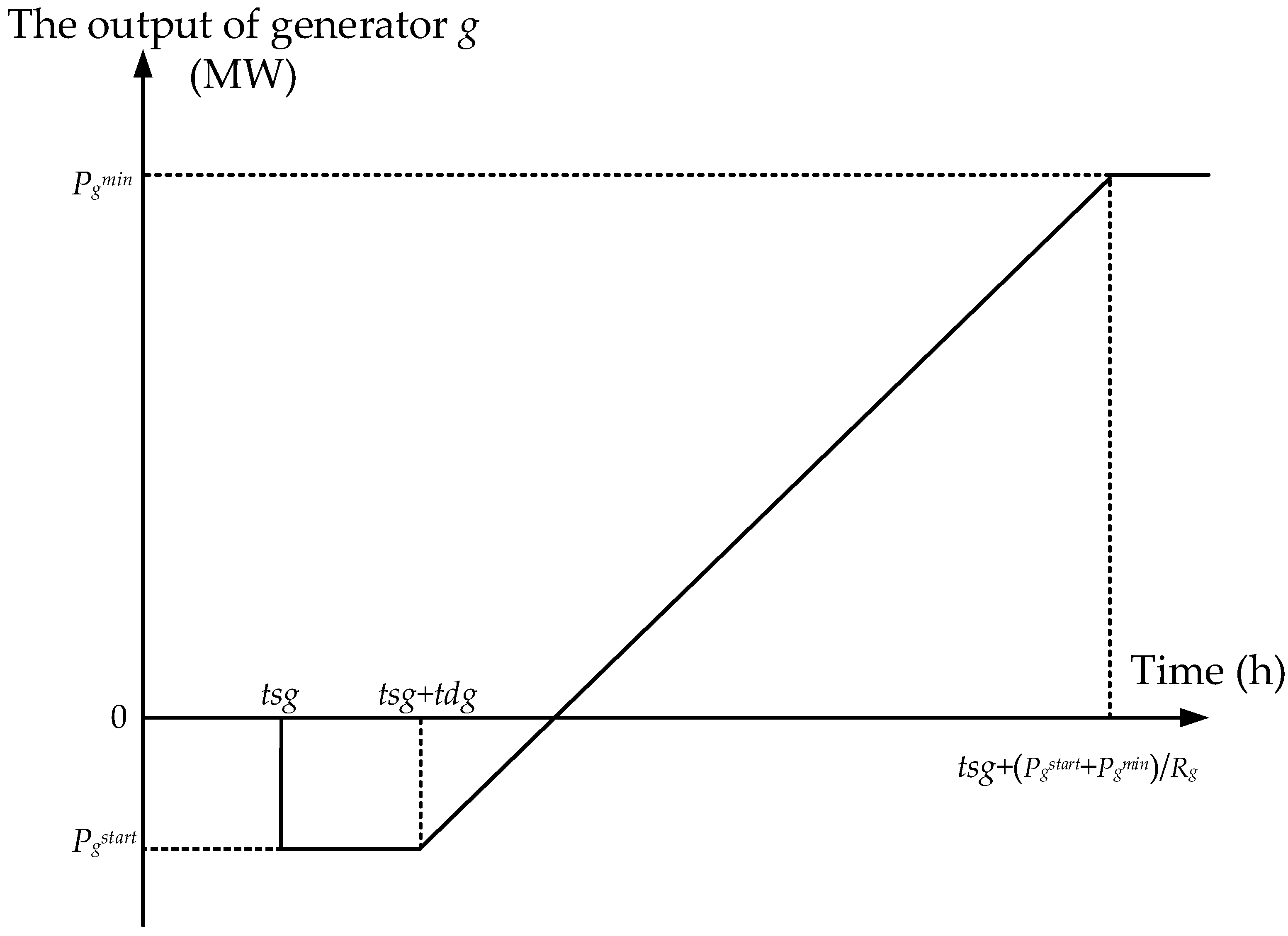
- The restoration characteristic of generators
The damage of bus will result in the outage of generators on it and these generators will not be started up until the bus is repaired. If SSg,tsg equals to 1, unit g is started up at tsg, as shown in Figure 2 [33]. Once the generator is started up, it has to absorb power from the power system (without considering generators with black start ability). Then the generator has the capability to transmit power to the system after its auxiliary power is self-sufficient. The simplified restoration process of generators is shown in (34)–(39).
If the generator is started up at tsg, in the interval 0~tsg, the output of the generator is 0, as shown in (34); constraint (35) indicates that the unit will absorb Pgstart power to start for time tdg; then the power absorbed by the unit is decreased gradually and it begins to transmit power to the system, as shown in (36). The ramp speed of generators is limited by (37). Constraints (38) and (39) define the active and reactive power output limits.
- Constraints of component operation states
The operation state variable BSi,t of bus i at time t equals to 1 if the bus is neither damaged nor under repair, as shown in (40). Constraint (41) indicates that the available state variable ALSij,t of line i→j at time t equals to 1 if the line and its linked buses are normal. Constraint (42) presents that the available state ALSij,t of the undamaged line i→j is determining by BSi,t and BSj,t. As for the operation state of line i→j, LSij,t is 0 when ALSij,t equals to 0 and 1 or 0, according to the decision of system dispatchers when ALSij,t equals to 1, as expressed by (43).
Besides, the operation state variable GSg,t of unit g at time t equals to 1 if the unit is neither damaged nor under repair, as shown in (44). If the unit is on a damaged bus, the state of the unit follows that of the bus, which is expressed by (45). In addition, constraint (46) presents the start-up state of unit g. If GSg,t is 1 and GSg,t−1 is 0, it means that the unit g is started up at time t, which is designated by SSg,t.
3.2.3. Coupling Constraints
The fault repair route problem and the post-disaster power system operation problem can be extracted from the above constraints. When components are damaged or under repair, they cannot be put into operation and will influence the topology of power systems. Therefore, the two problems are coupled by the following coupling constraints.
If BSx,t is 0, all lines connected to bus x are not available and the generators on bus x are out of service.
3.2.4. Transformation of Complex Nonlinear Constraint
The co-optimization model is established from (1)–(48). However, the model is a non-convex and non-linear optimization problem, which is very difficult to solve directly. For the 0–1 variable ALSij,t, which is the multiplication of two binary variables, it can be linearized by (49). Thus, the complex nonlinear constraint (42) is transformed to linear constraints. As a result, the original model is converted to a MISOCP, which relatively reduces the computational complexity.
4. Solution
Though the original model is transformed to a MISOCP, it is still a large-scale and complex problem, which is hard for ordinary solvers to solve. The LR method is a decomposition and coordination algorithm and its computational effort increases linearly with the scale of problem, so it is suitable for the solution of the modified model. The MISOCP model can be decomposed into the upper sub problem of routing repair teams and the lower sub problem of power system operation optimization by LR and then calculated by iterative solution. Further, to tackle the concussion and slow convergence of LR, the acceleration strategy is designed to speed up the solving process.
4.1. Lagrange Relaxation of the MISOCP Model
In this part, the coupling constraints of the MISOCP model are relaxed and added into the objective function. Only simple constraints (uncoupling constraints) are left and the MISOCP model is decoupled into two sub problems by LR. The objective function is converted to the following form:
which equals to
λl,t and λb,t are Lagrange multipliers of constraints (47) and (48) respectively.
It is easy to see that the former part relates to the route and working time of repair teams, while the latter part only relates to states of system components and outputs of units. The upper sub problem of damage repair routing and the lower sub problem of power system operation optimization are further formulated.
- The damage repair routing problem
Constraints (2)–(17).
- The power system operation optimization problem
Constraints (18)–(41), (43)–(46) and (49).
Subsequently, the two problems are solved alternatively and Lagrange multipliers are updated to achieve co-optimization. In this paper, the multipliers are updated by the surrogate gradient method [34] and their updating process follows these rules.
where wup and wdown are positive numbers, which represent the increase or decrease steps of multipliers separately.
The value of duality gap is used as the LR convergence criterion, that is,
where γ is the objective function value of the original model, which can be calculated by constraint (1); β is the objective function value of the relaxed model, which can be calculated by constraint (50).
4.2. The Acceleration Strategy
LR tends to oscillate during the convergence procedure, increasing the number of iterations and prolonging computing time. Thus, the acceleration strategy is designed to speed up the solving process, which helps to get an approximate optimal solution quickly.
The upper limit of iteration number (Nul) and the maximum number of violated coupling constraints (Nmv) should be set by decision makers. When the iteration number reaches Nul, or the number of violated coupling constraints reaches Nmv, the acceleration strategy is activated. Under this circumstance, the sub problem of damage repair routing is solved first according to Lagrange multipliers obtained from the last iteration. Then, the sub problem of power system operation optimization is solved based on the results of damage repair routing.
4.3. The Algorithm Flow
The flow chart of the acceleration algorithm proposed in this paper is shown in Figure 3. Its solution process is listed as below.
- The original co-optimization model is transformed to the modified MISOCP model by linearizing some complex constraints.
- Set the initial values of Lagrange multipliers.
- The MISOCP model is decomposed into the upper sub problem of damage repair routing and the lower sub problem of power system operation optimization.
- Solve the two sub problems alternately in each iteration. If the LR convergence criterion is satisfied, output the result and end the calculation or else go to step 5.
- If the acceleration convergence condition is satisfied, implement the acceleration strategy and output the result. Otherwise, update the values of Lagrange multipliers and go to step 4.
The advantages of the LR-based algorithm are as follows.
(1) The NP-hard problems are difficult to solve due to the optimization of integer variables. LR helps to distribute integer variables to different problems and enhance the solving efficiency. Besides, at the expense of increasing the number of iterations, the overall scale of the problem is reduced, making large-scale problems solvable.
(2) The algorithm makes the physical meanings of the co-optimization more concise. After LR, the model is separated into the damage repair routing problem and the power system operation problem, which are more conformable to the actual work of the maintenance department and the power system dispatching department. For utilities, once the power system is hit by disasters, the maintenance department acquires the information of components states, fault points locations and repair resources and then formulate the best damage repair routes. Power system dispatchers only have to care about the operation cost of generators, the switching of lines and the load shedding situation. Based on independent decision making, the two departments are restricting each other by Lagrange multipliers to achieve the best economic benefit of the entity. The work efficiency is greatly improved as well.
5. Case Study
The co-optimization model is tested on the IEEE 57-bus test system [35], to demonstrate the effectiveness of the model. The computer used is with Intel Core i7-6700 3.40 GHz CPU and 8 GB RAM. The problems are modeled in MATLAB R2014a and solved by Gurobi 7.0.2.
In the case study, it is assumed that the power system is hit and disturbed by a severe typhoon. The damage locations of the post-disaster power system are known, as shown in Figure 4. The distance between different fault points, the distance between fault points and repair centers, the needed damage repair resources and time of fault points, the resource amount of repair centers and the economic loss of lost load are displayed from Table A1, Table A2, Table A3, Table A4 and Table A5 in Appendix A.
The time length of restoration horizon T is 40 h. An hourly simulation step is adopted. From [36,37], the economic loss of lost load is divided into four categories: $10/kWh for the most important load, $6.979/kWh for important load, $3.706/kWh for ordinary load and $0.110/kWh for least important load. Each repair team consists of 5 members and the average wage of each member is assumed to be $70/h. The gas cost for each team is $33/100 km. The average driving speed of each team is 50 km/h. Rating of each transmission line is 100 MVA. Bus voltage limit is [0.94, 1.06]. The maximum number of violated coupling constraints (Nmv) is 6. The weights in the objective function are set to be α1 = 1, α2 = 1 and α3 = 10, to highlight the importance of reducing the power outage loss.
To improve the computational efficiency, the clustering method proposed in [30] is used to acquire repair assignments of each repair center. The objective of the clustering model is to minimize the sum of the distances between repair centers and fault points which they are responsible for. It should be guaranteed that each fault component is repaired and each repair center has enough resources to finish its tasks. The clustering result is listed in Table 1, while 1 indicates the damaged component will be repaired by the repair center and 0 else.
5.1. The Advantage Analysis of the Proposed Co-Optimization Model
Two cases are designed in this part to prove the advantages of the proposed co-optimization model.
Case 1: the damage repair scheme and the power system operation optimization are co-optimized using the proposed method.
Case 2: the damage repair scheme is formulated independently to realize the minimization of the repair expenses. Then, according to the damage repair scheme and the available states of system components, the power system operation optimization is conducted to minimize the power generation cost and power outage loss.
The repair routes with and without co-optimization are shown in Figure 5 and Figure 6. The arrival moments at each damaged component with and without co-optimization are listed in Table 2 and Table 3.
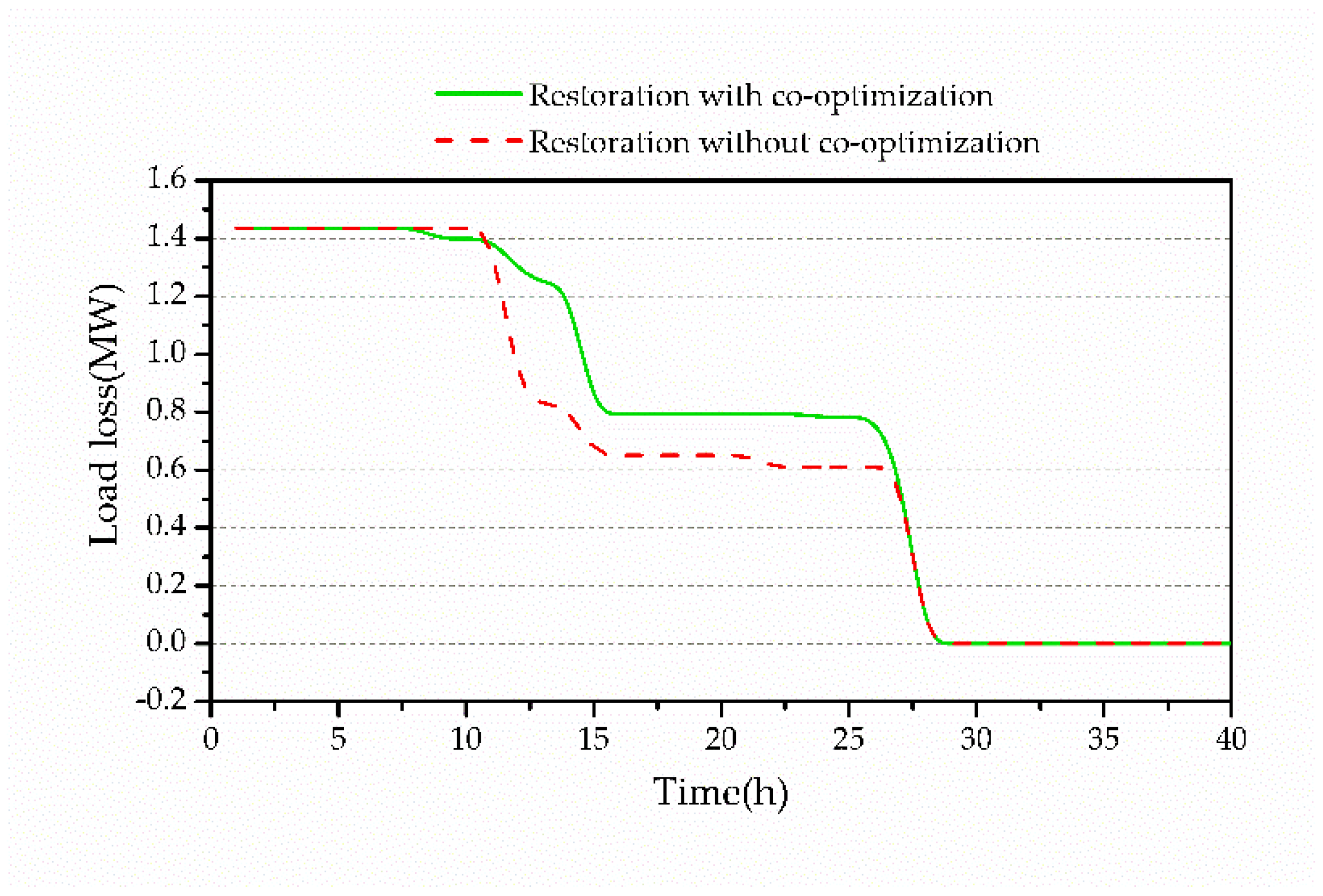
The economic indices with and without co-optimization are depicted in Table 4. The power outage economic loss and the load loss with and without co-optimization are shown in Figure 7 and Figure 8.
When the power system is restored without co-optimization, the expense of damage repair will be lower whereas the outage loss is higher. Moreover, though the restoration without co-optimization reduces the total load loss, it cannot ensure the quick restoration of the important load. By contrast, if the damage repair is co-optimized with power system operation problem, the power outage loss will be greatly reduced, especially for the most important load, which will bring more obvious social benefits and accord better with requirements of the post-disaster power system restoration. Hence, the results demonstrate that the effectiveness and necessity of the proposed co-optimization model for post-disaster power system restoration.
5.2. The Effect Analysis of the Acceleration Algorithm
The computational performance of different solving methods is shown in Table 5.
It is observed that since the original model is a large-scale non-convex and non-linear optimization problem and the direct approach cannot converge to a feasible solution. Though the modified MISOCP model can be solved directly, the computation time is long, which does not meet the actual demand for rapid restoration of post-disaster power systems. However, the convergence speed of the MISOCP model can be greatly accelerated when the model is solved by the LR-based algorithm. Besides, the restoration economic loss and cost of the MISOCP model with and without the acceleration algorithm are approximately equal. That is, the acceleration algorithm can ensure the accuracy of the solution and improve the computational efficiency.
5.3. The Impacts of Damage Repair Resources Allocation and Adequacy on Restoration
The economic impact of repair resources allocation and adequacy on restoration is analyzed. The resource amount of repair centers is changed. When the resource amount available of the three repair centers is 50, 100 and 60 respectively, the power outage loss rises from $803,380 to $865,624 and the repair cost rises $53,320 from to $57,607, as shown in Table 6. What’s more, some damaged components cannot be repaired within 40 h after the beginning of the restoration process and it takes longer time to restore all outage load than the original resource allocation case.
Therefore, the adequacy and allocation of repair resources will have significant effect on power system restoration. The inadequate or irrational allocation of resources will increase the loss of power outage and extend the duration of power restoration. Consequently, it is crucial to identify the possible areas disturbed by disasters in advance and distribute enough repair resources to damage repair centers, guaranteeing the post-disaster fast repair of fault points.
5.4. The Impacts of Weight Factors in the Objective Function on Restoration
The impacts of weight factors in the objective function on the power system restoration is studied. Four combinations of weight factors are analyzed and the results are listed in Table 7.
In the previous analysis, α1 = 1, α2 = 1 and α3 = 10, as mentioned above. With this setting, the restoration work of lost load is prioritized, reducing the power shortage cost. When α3 is reduced along with the increase of α1 and α2, though the repair cost and operation cost of the restoration process have been reduced, the power outage loss has increased. Especially, if we select α1 = 10, α2 = 1 and α3 = 1 to highlight the expense of power system operation, the system operation cost is decreased by about $380,000; however, the power outage loss is sharply increased by about $1,100,000. Therefore, the values of weight factors in the objective function have great influence on the restoration effect. Generally, the most critical task after disasters is to restore the outage load and decrease power loss of users, so the repair cost and system operation cost should not be important concerns for decision makers. Hence, it is essential to set larger weight for α3.
6. Conclusions
In this paper, a co-optimization model was proposed for the post-disaster power system restoration work and the enhancement of resilience. The model can optimally coordinate the damage repair work with power system operation. Additionally, the original model is converted to a MISOCP model and the algorithm based on Lagrange relaxation is proposed to accelerate the calculation speed. The case study demonstrates the effectiveness of the co-optimization model and the algorithm. Besides, the specific conclusions are drawn as follows.
- The proposed model can support the formulation of reasonable damage repair scheme, the plan of unit output and the decisions of optimal transmission switching, to minimize the power outage loss with lower cost of damage repair and power system operation.
- Lagrange relaxation decomposes the original complex model into two small-scale sub problems and the acceleration strategy is implemented to realize the fast solution. For utilities, the work of maintenance department and system dispatching department could be separated and Lagrange multipliers help to coordinate their work. Consequently, the work efficiency will be improved.
- The adequacy and allocation of damage repair resource can greatly influence the restoration effect and the load loss level. The sufficient resource reserve of repair centers will significantly decrease loss in economy due to power outage.
- To reduce the power outage loss and realize the enhancement of post-disaster power system resilience, it is significant to highlight the fast restoration of outage loads according to their importance.
Future work will further improve the computational efficiency of the developed model and test the model on real-world and large-scale systems.
Author Contributions
H.Z. and G.L. conceived and designed the study. H.Z. and H.Y. wrote the paper.
Funding
This work was funded by the National Natural Science Foundation of China (51577147) and Science and Technology Project of State Grid, China (5202011600UG).
Acknowledgments
Student Chao Yan helped to polish the paper.
Conflicts of Interest
The authors declare no conflict of interest.
Nomenclature
| Indices and sets | |
| g | Index for generation units |
| i/j | Index for buses |
| x/y/z | Index for damaged components |
| c | Index for repair team |
| t | Index for time |
| b | Index for repair center (starting point) |
| d | Index for repair center (return point) |
| DC | Set of damaged components |
| DB | Set of damaged buses |
| DL | Set of damaged transmission lines |
| Parameters | |
| α | Weight factor |
| ag | Generation cost quadric coefficient of unit g |
| bg | Generation cost linear coefficient of unit g |
| cg | Generation cost constant of unit g |
| lpi,t/lqi,t | Active/reactive demand at bus i and time t under normal conditions |
| eli | Economic loss of lost load at bus i per hour |
| Gi/Bi | Conductance/susceptance from bus i to the ground |
| Vimax/Vimin | Upper/lower limit of voltage magnitude at bus i |
| θimax/θimin | Upper/lower limit of voltage angle at bus i |
| Pgmax/Pgmin | Upper/lower limit of active power generation of unit g |
| Qgmax/Qgmin | Upper/lower limit of reactive power generation of unit g |
| Pgstart | Power required by unit g for start-up |
| Rg | Ramp speed limit of unit g |
| tsg | Start-up time of unit g |
| tdg | The interval of unit g with positive start-up power requirement and zero ramping rate |
| Sij | Upper limit of apparent power flow on line i→j |
| Iijmax | Upper limit of current on line i→j |
| rij/xij | Resistance/reactance of line i→j |
| dx,y | Distance between damaged component x and y |
| Vc | Average driving speed of team c |
| Capc | Resource capacity of team c |
| RESx | Repair resources required to fix damaged component x |
| resd | Resource amount of repair center |
| RTx,c | Repair time required to fix damaged component x |
| Numc | Number of repair teams |
| M | Value of big M |
| T | Time horizon |
| ωcrew | Wages of a repair team per hour |
| ωroad | Driving cost of a repair team per km |
| Variables | |
| PGg,t/QGg,t | Active/reactive power generation of unit g at time t |
| PLij,t/QLij,t | Active/reactive power flow on line i→j |
| hij,t | Square of current magnitude on line i→j at time t |
| LPi,t/LQi,t | Actual active/reactive load at bus i and time t |
| Vi,t | Voltage magnitude at bus i and time t |
| θi,t | Voltage phase at bus i and time t |
| ALSij,t | Binary variable equals to 0 if line i→j is damaged or under repair and 1 else at time t |
| LSij,t | Binary variable equals to 0 if line i→j is removed from the system and 1 else at time t |
| BSi,t | Binary variable equals to 0 if bus i is damaged or under repair and 1 else at time t |
| GSg,t | Binary variable equals to 1 if unit g is committed and 0 else at time t |
| SSg,t | Binary variable equals to 1 if unit g is started up at time t and 0 else |
| ATx,c | Arrival time of team c at damaged component x |
| FTx,t | Binary variable equals to 1 if damaged component x is repaired at time t and 0 else |
| Mx,y,c | Binary variable equals to 1 if team c moves from damaged component x to y and 0 else |
| Nx,c | Binary variable equals to 1 if damaged component x is repaired by team c and 0 else |
| Sx,t | Binary variable equals to 0 if damaged component x is damaged or under repair and 1 else at time t |
Appendix A

Table A1.
Distance (km) between fault points.
| Numbers of Damaged Components | Bus Number | Line Number | |||||||||
|---|---|---|---|---|---|---|---|---|---|---|---|
| 3 | 14 | 52 | 53 | 14 | 17 | 29 | 32 | 40 | 70 | ||
| Bus number | 3 | 0 | 345 | 840 | 870 | 375 | 450 | 60 | 120 | 735 | 975 |
| 14 | 345 | 0 | 915 | 900 | 45 | 135 | 225 | 195 | 1065 | 840 | |
| 52 | 840 | 915 | 0 | 90 | 885 | 1050 | 780 | 660 | 90 | 180 | |
| 53 | 870 | 900 | 90 | 0 | 855 | 1080 | 750 | 630 | 180 | 90 | |
| Line number | 14 | 375 | 45 | 885 | 855 | 0 | 165 | 330 | 285 | 900 | 930 |
| 17 | 450 | 135 | 1050 | 1080 | 165 | 0 | 375 | 345 | 1050 | 1065 | |
| 29 | 60 | 225 | 780 | 750 | 330 | 375 | 0 | 90 | 750 | 870 | |
| 32 | 120 | 195 | 660 | 630 | 285 | 345 | 90 | 0 | 705 | 690 | |
| 40 | 735 | 1065 | 90 | 180 | 900 | 1050 | 750 | 705 | 0 | 270 | |
| 70 | 975 | 840 | 180 | 90 | 930 | 1065 | 870 | 690 | 270 | 0 | |
Table A2.
Distance (km) between fault points and repair centers.
| Repair Center | Bus Number | Line Number | ||||||||
|---|---|---|---|---|---|---|---|---|---|---|
| 3 | 14 | 52 | 53 | 14 | 17 | 29 | 32 | 40 | 70 | |
| 1 | 780 | 885 | 90 | 82.5 | 810 | 1020 | 832.5 | 555 | 150 | 120 |
| 2 | 120 | 315 | 735 | 720 | 450 | 540 | 105 | 180 | 780 | 780 |
| 3 | 465 | 45 | 840 | 825 | 120 | 195 | 360 | 307.5 | 795 | 950 |
Table A3.
Damage repair resource and time of fault points.
| Damage Repair Requirements | Bus Number | Line Number | ||||||||
|---|---|---|---|---|---|---|---|---|---|---|
| 3 | 14 | 52 | 53 | 14 | 17 | 29 | 32 | 40 | 70 | |
| Damage repair resource | 30 | 28 | 34 | 32 | 8 | 11 | 9 | 14 | 6 | 7 |
| Damage repair time (h) | 12 | 13 | 12 | 14 | 8 | 7 | 9 | 10 | 6 | 8 |
Table A4.
Resource amount of repair centers.
| Repair Center | Resource (Capability of Each Team) |
|---|---|
| 1 | 85 (45; 45) |
| 2 | 60 (45; 45) |
| 3 | 60 (45; 45) |
Table A5.
Economic loss of lost load on load buses.
| Load Bus Number | Economic Loss of Lost Load ($/kWh) |
|---|---|
| 1 | 0.110 |
| 2 | 0.110 |
| 3 | 0.110 |
| 4 | 3.816 |
| 5 | 0.110 |
| 6 | 10.000 |
| 8 | 0.110 |
| 9 | 0.110 |
| 10 | 0.110 |
| 12 | 0.110 |
| 13 | 0.110 |
| 14 | 0.110 |
| 15 | 0.110 |
| 16 | 6.979 |
| 17 | 0.110 |
| 18 | 0.110 |
| 19 | 0.110 |
| 20 | 3.816 |
| 23 | 0.110 |
| 25 | 10.000 |
| 27 | 3.816 |
| 28 | 0.110 |
| 29 | 0.110 |
| 30 | 0.110 |
| 31 | 0.110 |
| 32 | 6.979 |
| 33 | 0.110 |
| 35 | 0.110 |
| 38 | 0.110 |
| 41 | 6.979 |
| 42 | 0.110 |
| 43 | 0.110 |
| 44 | 0.110 |
| 47 | 0.110 |
| 49 | 0.110 |
| 50 | 0.110 |
| 51 | 0.110 |
| 52 | 3.816 |
| 53 | 0.110 |
| 54 | 0.110 |
| 55 | 3.816 |
| 56 | 0.110 |
| 57 | 0.110 |
References
- Shao, D.; Yin, X.; Chen, Q.; Tong, G.; Zhang, Z.; Zheng, Y.; Hou, H. Affects of Icing and Snow Disaster Occurred in 2008 on Power Grids in South China. Power Syst. Technol. 2009, 33, 38–43. [Google Scholar]
- Bie, Z.; Lin, Y.; Li, G.; Li, F. Battling the Extreme: A Study on the Power System Resilience. Proc. IEEE 2017, 105, 1253–1266. [Google Scholar] [CrossRef]
- Smith, R. US Risks National Blackout from Small Scale Attack. Wall Street Journal. 12 March 2014. Available online: https://www.studentnewsdaily.com/daily-news-article/u-s-risks-national-blackout-from-small-scale-attack/ (accessed on 12 March 2014).
- Panteli, M.; Trakas, D.N.; Mancarella, P.; Hatziargyriou, N.D. Power Systems Resilience Assessment: Hardening and Smart Operational Enhancement Strategies. Proc. IEEE 2017, 105, 1202–1213. [Google Scholar] [CrossRef]
- Zhang, H.; Yuan, H.; Li, G. Quantitative Resilience Assessment under a Tri-Stage Framework for Power Systems. Energies 2018, 11, 1427. [Google Scholar] [CrossRef]
- Yuan, W.; Wang, J.; Qiu, F.; Chen, C.; Kang, C.; Zeng, B. Robust Optimization-Based Resilient Distribution Network Planning Against Natural Disasters. IEEE Trans. Smart Grid 2016, 7, 2817–2826. [Google Scholar] [CrossRef]
- Shao, C.; Shahidehpour, M.; Wang, X.; Wang, X.; Wang, B. Integrated Planning of Electricity and Natural Gas Transportation Systems for Enhancing the Power Grid Resilience. IEEE Trans. Power Syst. 2017, 32, 4418–4429. [Google Scholar] [CrossRef]
- Arab, A.; Khodaei, A.; Khator, S.K.; Ding, K.; Emesih, V.A.; Han, Z. Stochastic pre-hurricane restoration planning for electric power systems infrastructure. IEEE Trans. Smart Grid 2015, 6, 1046–1054. [Google Scholar] [CrossRef]
- Lin, Y.; Bie, Z. Tri-level optimal hardening plan for a resilient distribution system considering reconfiguration and DG islanding. Appl. Energy 2018, 201, 1266–1279. [Google Scholar] [CrossRef]
- Tan, Y.; Das, A.K.; Arabshahi, P.; Kirschen, K.S. Distribution Systems Hardening against Natural Disasters. IEEE Trans. Power Syst. 2017, 99. [Google Scholar] [CrossRef]
- Zhang, B.; Dehghanian, P.; Kezunovic, M. Optimal Allocation of PV Generation and Battery Storage for Enhanced Resilience. IEEE Trans. Smart Grid 2017, 99. [Google Scholar] [CrossRef]
- Gao, H.; Chen, Y.; Mei, S.; Huang, S.; Xu, Y. Resilience-oriented pre-hurricane resource allocation in distribution systems considering electric buses. Proc. IEEE 2017, 105, 1214–1233. [Google Scholar] [CrossRef]
- Wang, Z.; Wang, J. Self-Healing Resilient Distribution Systems Based on Sectionalization into Microgrids. IEEE Trans. Power Syst. 2015, 30, 3139–3149. [Google Scholar] [CrossRef]
- Panteli, M.; Trakas, D.N.; Mancarella, P.; Hatziargyriou, N.D. Boosting the power grid resilience to extreme weather events using defensive islanding. IEEE Trans. Smart Grid 2017, 7, 2913–2922. [Google Scholar] [CrossRef]
- Pinto, R.T.; Aragüés-Peñalba, M.; Gomis-Bellmunt, O.; Sumper, A. Optimal operation of dc networks to support power system outage management. IEEE Trans. Smart Grid 2016, 7, 2953–2961. [Google Scholar] [CrossRef]
- Ding, T.; Lin, Y.; Li, G.; Bie, Z. A new model for resilient distribution systems by microgrids formation. IEEE Trans. Power Syst. 2017, 7, 2953–2961. [Google Scholar] [CrossRef]
- Gao, H.; Chen, Y.; Xu, Y.; Liu, C.C. Resilience-oriented critical load restoration using microgrids in distribution systems. IEEE Trans. Smart Grid 2016, 7, 2837–2848. [Google Scholar] [CrossRef]
- Francesco, E.; Leccese, F. Risks analysis for already existent electric lifelines in case of seismic disaster. In Proceedings of the International Conference on Environment and Electrical Engineering, Venice, Italy, 18–25 May 2012. [Google Scholar]
- Seneviratne, D.; Ciani, L.; Catelani, M. Smart maintenance and inspection of linear assets: An Industry 4.0 approach. ACTA IMEKO 2018, 7, 50–56. [Google Scholar] [CrossRef] [Green Version]
- Zhao, Y.; Lin, Z.; Ding, Y.; Liu, Y.; Sun, L.; Yan, Y. A Model Predictive Control Based Generator Start-Up Optimization Strategy for Restoration with Microgrids as Black-Start Resources. IEEE Trans. Power Syst. 2018, 99. [Google Scholar] [CrossRef]
- Sun, L.; Lin, Z.; Xu, Y.; Wen, F.; Zhang, C.; Xue, Y. Optimal skeleton-network restoration considering generator start-up sequence and load pickup. IEEE Trans. Smart Grid 2018, 99. [Google Scholar] [CrossRef]
- Patsakis, G.; Rajan, D.; Aravena, I.; Rios, J.; Oren, S. Optimal black start allocation for power system restoration. IEEE Trans. Smart Grid 2018, 99. [Google Scholar] [CrossRef]
- Abbasi, S.; Barati, M.; Lim, G.J. A parallel sectionalized restoration scheme for resilient smart grid systems. IEEE Trans. Smart Grid 2017. [Google Scholar] [CrossRef]
- Liu, W.; Lin, Z.; Wen, F.; Chung, C.Y.; Xue, Y.; Ledwich, G. Sectionalizing strategies for minimizing outage durations of critical loads in parallel power system restoration with bi-level programming. Int. J. Electr. Power. 2015, 71, 327–334. [Google Scholar] [CrossRef]
- Zhao, J.; Wang, H.; Liu, Y.; Azizipanah-Abarghooee, R.; Terzija, V. Utility-Oriented On-Line Load Restoration Considering Wind Power Penetration. IEEE Trans. Sustain. Energy 2018, 99. [Google Scholar] [CrossRef]
- Wang, C.; Vittal, V.; Sun, K. Obdd-based sectionalizing strategies for parallel power system restoration. IEEE Trans. Power Syst. 2011, 26, 1426–1433. [Google Scholar] [CrossRef]
- Qin, Z.; Hou, Y.; Liu, C.C.; Liu, S. Coordinating generation and load pickup during load restoration with discrete load increments and reserve constraints. IET Gener. Transm. Distrib. 2015, 9, 2437–2446. [Google Scholar] [CrossRef]
- Hentenryck, P.V.; Coffrin, C.; Bent, R. Vehicle routing for the last mile of power system restoration. In Proceedings of the 17th Power Systems Computation Conference (PSCC), Stockholm, Sweden, 22–26 August 2011. [Google Scholar]
- Simon, B.; Coffrin, C.; Hentenryck, P.V. Randomized adaptive vehicle decomposition for large-scale power restoration. In Proceedings of the International Conference on Integration of Ai and or Techniques in Constraint Programming for Combinatorial Optimization Problems, Nantes, France, 28 May–1 June 2012. [Google Scholar]
- Arif, A.; Wang, Z.; Wang, J.; Chen, C. Power distribution system outage management with co-optimization of repairs, reconfiguration, and DG dispatch. IEEE Trans. Smart Grid 2017. [Google Scholar] [CrossRef]
- Wood, A.J.; Wollenberg, B.F. Power Generation, Operation, and Control, 2nd ed.; Wiley, Inc.: New York, NY, USA, 1996; ISBN 978-0-471-58699-9. [Google Scholar]
- Bai, Y.; Zhong, H.; Xia, Q.; Wang, Y. A conic programming approach to optimal transmission switching considering reactive power and voltage security. In Proceedings of the Power & Energy Society General Meeting, Denver, CO, USA, 26–30 July 2015. [Google Scholar]
- Hou, Y.; Liu, C.C.; Sun, K.; Zhang, P.; Liu, S.; Mizumura, D. Computation of milestones for decision support during system restoration. IEEE Trans. Power Syst. 2011, 26, 1399–1409. [Google Scholar] [CrossRef] [Green Version]
- Zhao, X.; Luh, P.B.; Wang, J. Surrogate gradient algorithm for lagrangian relaxation. J. Optim. Theory Appl. 1999, 100, 699–712. [Google Scholar] [CrossRef]
- Power System Test Case Archive; Department of Electrical Engeneering, University of Washington: Seattle, WA, USA, 2007; Available online: https://www2.ee.washington.edu/research/pstca/pf57/pg_tca57bus.htm (accessed on 7 August 2018).
- London Economics International LLC. Estimating the Value of Lost Load; Electricity Reliability Council of Texas Inc., London Economics International (LLC): Boston, MA, USA, 2013. [Google Scholar]
- Arab, A.; Khodaei, A.; Khator, S.K.; Han, Z. Electric Power Grid Restoration Considering Disaster Economics. IEEE Access 2016, 4, 639–649. [Google Scholar] [CrossRef]
Figure 1.
The illustrative process of a resilient power system under disasters.

Figure 2.
The restoration process of generators without black start ability.

Figure 3.
The flow chart of the acceleration algorithm.

Figure 4.
The damage locations of the post-disaster IEEE 57-bus test system.
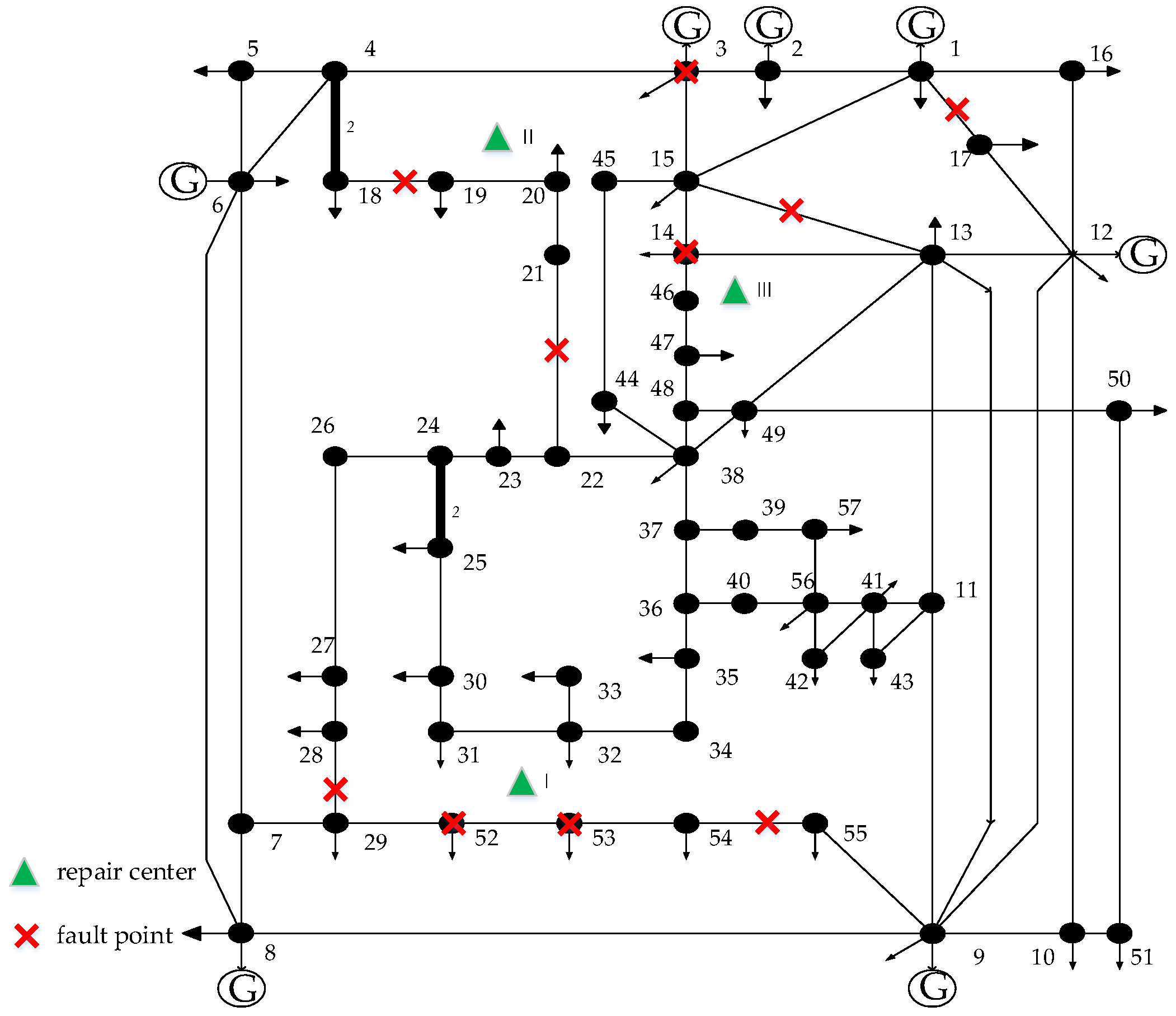
Figure 5.
The repair routes with co-optimization.

Figure 6.
The repair routes without co-optimization.
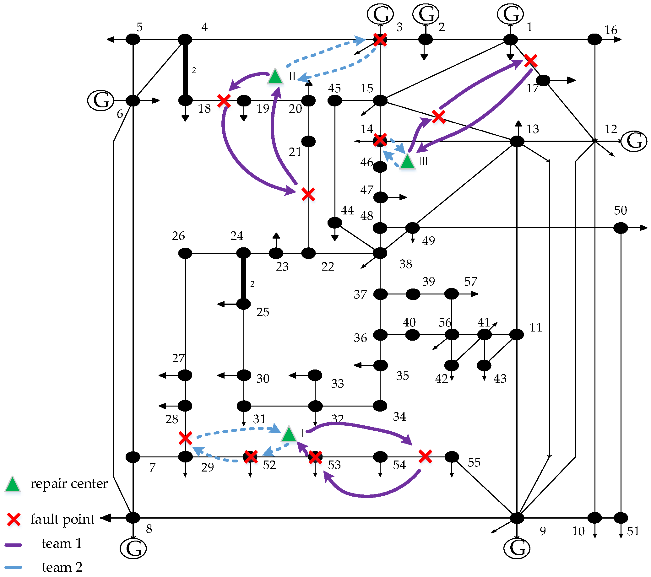
Figure 7.
The power outage economic loss with and without co-optimization.

Figure 8.
The load loss with and without co-optimization.

Table 1.
Damage repair assignment for each repair center.
| Repair Center | Bus Number | Line Number (Bus i–Bus j) | ||||||||
|---|---|---|---|---|---|---|---|---|---|---|
| 3 | 14 | 52 | 53 | 14(13–15) | 17(1–17) | 29(18–19) | 32(21–22) | 40(28–29) | 70(54–55) | |
| 1 | 0 | 0 | 1 | 1 | 0 | 0 | 0 | 0 | 1 | 1 |
| 2 | 1 | 0 | 0 | 0 | 0 | 0 | 1 | 1 | 0 | 0 |
| 3 | 0 | 1 | 0 | 0 | 1 | 1 | 0 | 0 | 0 | 0 |
Table 2.
The arrival time at each damaged component with co-optimization.
| Damaged Component | Bus Number | Line Number | ||||||||||
|---|---|---|---|---|---|---|---|---|---|---|---|---|
| 3 | 14 | 52 | 53 | 14 | 17 | 29 | 32 | 40 | 70 | |||
| Arrival moment (h) | Repair center 1 | Team 1 | - | - | 1.8 | - | - | - | - | - | - | 15.6 |
| Team 2 | - | - | - | 12.2 | - | - | - | - | 2.4 | - | ||
| Repair center 2 | Team 1 | - | - | - | - | - | - | 2.1 | 12.9 | - | - | |
| Team 2 | 14.0 | - | - | - | - | - | - | - | - | - | ||
| Repair center 3 | Team 1 | - | - | - | - | 14.2 | 3.9 | - | - | - | - | |
| Team 2 | - | 0.9 | - | - | - | - | - | - | - | - | ||
Table 3.
The arrival time at each damaged component without co-optimization.
| Damaged Component | Bus Number | Line Number | ||||||||||
|---|---|---|---|---|---|---|---|---|---|---|---|---|
| 3 | 14 | 52 | 53 | 14 | 17 | 29 | 32 | 40 | 70 | |||
| Arrival moment (h) | Repair center 1 | Team 1 | - | - | - | 12.2 | - | - | - | - | - | 2.4 |
| Team 2 | - | 1.8 | - | - | - | - | - | 15.6 | - | |||
| Repair center 2 | Team 1 | - | - | - | - | - | - | 2.1 | 12.9 | - | - | |
| Team 2 | 2.4 | - | - | - | - | - | - | - | - | - | ||
| Repair center 3 | Team 1 | - | - | - | - | 2.4 | 13.7 | - | - | - | - | |
| Team 2 | - | 0.9 | - | - | - | - | - | - | - | - | ||
Table 4.
The economic indices with and without co-optimization.
| Economic Index | Restoration with Co-Optimization | Restoration without Co-Optimization |
|---|---|---|
| Damage repair expense ($1000) | 53.32 | 47.90 |
| System operation cost ($1000) | 1741.14 | 1750.21 |
| Power outage loss ($1000) | 803.38 | 967.55 |
Table 5.
The computational performance of different solving methods.
| Model | The Original Model | The MISOCP Model | The MISOCP Model+ the Acceleration Algorithm |
|---|---|---|---|
| Computation time | Did not converge | 22.5 h | 4.6 h |
| The objective function value | - | 9802.31 | 9828.24 |
Table 6.
The economic indices with and without co-optimization.
| Economic Index | The Original Resource Allocation Case | The Changed Resource Allocation Case |
|---|---|---|
| Damage repair expense ($1000) | 53.32 | 57.61 |
| Power outage loss ($1000) | 803.38 | 865.62 |
Table 7.
The economic indices for different weight factors.
| α1 | α2 | α3 | Power Outage Loss ($1000) | System Operation Cost ($1000) | Damage Repair Expense ($1000) |
|---|---|---|---|---|---|
| 1 | 1 | 10 | 803.38 | 1741.14 | 53.32 |
| 1 | 1 | 1 | 833.47 | 1695.92 | 49.25 |
| 10 | 1 | 1 | 1930.08 | 1361.93 | 54.79 |
| 1 | 10 | 1 | 883.23 | 1696.17 | 51.20 |
© 2018 by the authors. Licensee MDPI, Basel, Switzerland. This article is an open access article distributed under the terms and conditions of the Creative Commons Attribution (CC BY) license (http://creativecommons.org/licenses/by/4.0/).
Share and Cite
MDPI and ACS Style
Zhang, H.; Li, G.; Yuan, H. Collaborative Optimization of Post-Disaster Damage Repair and Power System Operation. Energies 2018, 11, 2611. https://doi.org/10.3390/en11102611
AMA Style
Zhang H, Li G, Yuan H. Collaborative Optimization of Post-Disaster Damage Repair and Power System Operation. Energies. 2018; 11(10):2611. https://doi.org/10.3390/en11102611
Chicago/Turabian StyleZhang, Han, Gengfeng Li, and Hanjie Yuan. 2018. "Collaborative Optimization of Post-Disaster Damage Repair and Power System Operation" Energies 11, no. 10: 2611. https://doi.org/10.3390/en11102611
Note that from the first issue of 2016, this journal uses article numbers instead of page numbers. See further details here.