Designing, Developing, and Implementing a Forecasting Method for the Produced and Consumed Electricity in the Case of Small Wind Farms Situated on Quite Complex Hilly Terrain

Abstract

Accurate forecasting of the produced and consumed electricity from wind farms is an essential aspect for wind power plant operators. In this context, our research addresses small-scale wind farms situated on hilly terrain, with the main purpose of overcoming the low accuracy limitations arising from the wind deflection, caused by the quite complex hilly terrain. A specific aspect of our devised forecasting method consists of incorporating advantages of recurrent long short-term memory (LSTM) neural networks, benefiting from their long-term dependencies, learning capabilities, and the advantages of feed-forward function fitting neural networks (FITNETs) that have the ability to map between a dataset of numeric inputs and a set of numeric targets. Another specific element of our approach consists of improving forecasting accuracy by means of refining the accuracy of the weather data input parameters within the same weather forecast resolution area. The developed method has power plant operators as main beneficiaries, but it can also be successfully applied in order to assess the energy potential of hilly areas with deflected wind, being useful for potential investors who want to build this type of wind farms. The method can be compiled and incorporated in the development of a wide range of customized applications targeting electricity forecasting for small wind farms situated on hilly terrain with deflected wind. The experimental results, the implementation of the developed method in a real production environment, its validation, and the comparison between our proposed method and other ones from the literature, confirm that the developed forecasting method represents an accurate, useful, and viable tool that addresses a gap in the current state of knowledge regarding the necessity for an accurate forecasting method that is able to predict with a high degree of accuracy both the produced and consumed electricity for small wind power plants situated on quite complex hilly terrain with deflected wind.

1. Introduction

1.1. Motivation

Renewable energy consists of all those virtually inexhaustible types of energy that are constantly regenerating in relatively short timeframes within certain natural processes, having the main advantage of being nonpolluting and environmentally friendly. Nowadays, one of the most serious problems faced by humanity is the continuing increase of environmental pollution caused mainly by the energy generation using classic fossil fuels (oil, coal, and natural gas). This is the reason why in the last decades, there can be observed a growing concern among scientists and governments for the implementation of renewable energies, resulting in increased investments in this type of plants.

The main types of renewable energy are wind, solar, water, geothermal, and biomass. Renewable energy brings many advantages as it does not produce emissions, conserves the natural reserves of the soil, reduces the level of water and soil pollution, creates jobs, and generates income for local communities. Since the usage of renewable energy offers many advantages, in many countries governments are currently encouraging the usage of this type of energy on a wider scale. The use of energy produced from renewable sources creates the foundations for ensuring energy security, saving traditional resources, reducing energy imports, developing the economy at all levels (local, regional, and global), and creating new labor market offers as well as reducing the environment pollution. When analyzing the increasing use of renewable energy, one should take into account a number of additional factors, such as the continuing increase of the global energy demand, caused by the economic expansion and global human population growth [1]. However, recently an economic crisis has reduced energy demand, but the consideration is acceptable on a wider timeframe.

At the global level, renewable energy resources are becoming increasingly popular, being influenced to a great extent by the evolving legislation and energy policies implemented by government and nongovernment authorities. For this purpose, the European Union (EU) aims to achieve constant progresses in order to attain a decarbonized environment in the years to come. The statement of the European Commission made on 14 June 2018 mentions that a political agreement has been reached among representatives of the European Commission, European Parliament, and the European Council regarding the increase of renewable energy usage in Europe. The updated, ambitious target concerning renewable energy sharing that must be reached by the year 2030 for the European Union has been set to a value of 32%, being also specified by a revision clause by the year 2023 in view of assessing the possibility to further increase the renewable energy share target [2].

Wind energy has been enticing a lot of interest for the last several decades as a result of its noteworthy characteristics, like extensive availability and wide range distribution with regard to other renewable energy resources. According to the Global Wind Energy Council (GWEC), the wind power market at the global level continued to stay above 50 GW in the year 2017, while Europe, India, and the offshore wind power sector having registered record years. The GWEC reports that the total wind power installations reached 52,492 MW in 2017, therefore determining a global total of 539,123 MW [3].

The report also points out that, actually, the annual wind power market was down 3.8% when compared to the value of 54,642 MW corresponding to the year 2016, but the cumulative total raised 11% when compared to the year-end total of the year 2016 that registered a total wind power of 487,279 MW. Even if the offshore wind power sector holds a market share of only 8% from the global wind power annual market and amounts to approximately 3.5% of the cumulative installed wind power capacity, one can state, without a doubt, that the offshore sector experiences quick growth. The report mentions that when compared to the year 2016, the offshore segment has increased by 87%, registering 4335 MW of wind power installations, and a 30% growth in the cumulative wind power capacity, therefore 2017 was a record year in this respect [3].

According to the 67th edition of the BP Statistical Review of World Energy from June 2018, worldwide renewable power has grown with an amount of 69.4 tons of oil equivalent in 2017 when compared to the previous year, the ton of oil equivalent (toe) representing the amount of energy that is released by burning one tone of crude oil. Therefore, renewable power has increased by 17%, which represents an increment record in the last 10 years. More than 50% of this growth is due to wind power [4]. After analyzing all of the presented figures, one can state that wind energy experiences a rapid evolution towards a complete profitable technology that has the potential of not relying on subsidies (like it currently benefits from) in the future, being able to compete in the marketplace with technologies that are burdened with taxes, like fossil fuels.

A major challenge for electricity market operators is extending the implementation of the renewable energy in general, and of the wind energy in particular, as they have to cope with the variable nature and uncertainty surrounding the generation of this type of energy, thus having to make certain decisions related to the amount of delivered energy. With regards to what concerns wind power, in order to manage its variable nature appropriately and ensure efficient operation of the related equipment, a very important aspect is the Wind Power Forecasting (WPF). At the same time, wind energy has a strong impact on the daily and hourly prices in the energy market, as the accurate forecasting of the variation of this type of energy significantly influences the compensation prices for the energy resources and for the energy that has been retained for future use.

In the following, we present a literature review in order to contextualize the current state of knowledge in which we position our paper and identify the gap that our proposed method addresses.

1.2. Literature Review

Analysis of the scientific literature reveals the fact that a series of papers in the field of energy address issues related to wind energy or to the forecast of produced wind energy on the basis of meteorological data.

López et al. [5] propose an artificial neural network model that combines the features of two types of Recurrent Neural Networks (RNNs) to forecast wind power from 1 to 48 steps ahead. The developed method consists in an Echo State Artificial Neural Network (ESN)-type architecture comprising an input layer, a hidden layer, and an output layer. López et al. used long short-term memory blocks within the hidden layer and conducted the training process in two main stages. With regard to the hidden layer, López et al. trained the network using a descending gradient method over the course of one epoch, while for the output layer a regularized regression was used in order to adjust it.

Xu et al. [6] proposed an echo state artificial neural network (ESN) approach fused with the particle swarm optimization (PSO) and metaheuristic Tabu search algorithms with the aim of improving the prediction accuracy of wind power forecasting by overcoming the drawbacks of the standard ESN. Xu et al. proposed this method for ultrashort-term or short-term forecasting horizons for the purpose of enhancing the electricity generation plan, diminishing the abandonment of wind power sites due to lack of appropriate forecasting tools, making appropriate adjustments to the maintenance schedule, and for facilitating the development of monitoring systems that operate in real time. As a consequence, Xu et al. state that their proposed method is superior to the standard ESN and Back Propagation (BP) neural network.

Cheng et al. [7] developed and presented an ensemble model comprising of wavelet threshold denoising (WTD), a RNN, and an adaptive neuro fuzzy inference system (ANFIS) for the purpose of probabilistic predicting of the wind speed. The forecasting horizon that their method targets is the ultra-short-term, namely for a one-hour-ahead wind speed prediction. Cheng et al. compared their ensemble model with other well-known machine learning approaches to forecast wind speed, taking into consideration four cases corresponding to different seasons. Cheng et al. claimed that their proposed ensemble model attains better forecasting accuracy of wind speed when compared to shallow ANNs (Artificial Neural Networks).

Wang et al. [8] proposed a hybrid prediction system that focuses on data preprocessing and uses extreme learning machine (ELM) techniques, enhanced by means of an employed cuckoo algorithm, in order to surpass the shortcomings of the standard ELM model. Wang et al. mentioned in their paper that they made use of the standard genetic algorithm in order to decrease the input’s dimensions and employ the autoregressive-moving-average model for correcting the errors, by targeting the enhanced ELM model.

Niu et al. [9] put forward a model that employs wavelet decomposition and weighted random forest enhanced by applying the niche immune lion algorithm, for the purpose of achieving an ultra-short-term forecasting horizon of wind power. Niu et al. mentioned that their proposed model benefits from the advantages brought by each of the individual employed models. After having analyzed two empirical cases, Niu et al. remarked that their devised model is superior to the back propagation artificial neural networks, support vector machines, random forest, and niche immune lion algorithm combined with random forest as it offered an excellent forecasting capability.

Boroojeni et al. [10] proposed a method for multi-time-scale modeling of the electric power demand forecasting, covering a time horizon from the short-term up to the medium-term, employing time-series with various cycles of seasonality from a power network, in order to model the historical load data. Boroojeni et al. developed their method to model separately the nonseasonal cycles of the load data and the seasonal cycles using two types of components: autoregressive and moving-average, relying on historical data regarding the load, without demanding historical data regarding the weather as additional inputs; this is a major advantage as the weather data are often unavailable. Boroojeni et al. evaluated the data modeling accuracy using two approaches: the first one is represented by classical computation of the forecasting errors, while the second one is based on using two information criteria, namely the Akaike and the Bayesian quantification methods characterized by the fact that they take into account the complexity of a model by penalizing it and the accuracy of the method by rewarding it. Boroojeni et al. showed that when the training set’s size or dimensions are modified, their model proves to be robust, while the forecasting error does not vary.

Yao et al. developed [11] a hybrid model combining wavelet denoising, a modified ant colony optimization algorithm, and Back Propagation neural networks. Yao et al. stated that their method is useful in predicting the wind speed for a short-term forecasting horizon based on a multistep approach. After developing the hybrid forecasting model, Yao et al. evaluated its accuracy using six real forecasting scenarios in order to highlight the forecasting accuracy, the stability of the developed model, and to confirm the usefulness of their method—considered by Yao et al. to be a tool designed for smart grid operators—in their planning and dispatching activities.

Zhao et al. [12] developed an algorithm for wind power forecasting that makes use of the Beveridge-Nelson, the Least Square Support Vector Machine, and the Grasshopper Optimization approaches. In the proposed multistage algorithm, the Beveridge-Nelson decomposition is used for breaking down the hourly wind electricity dataset in view of obtaining a deterministic trend and a cyclic term along with a random component. The Least Square Support Vector Machine method is enhanced by using the Grasshopper Optimization algorithm for forecasting 168 h ahead of the trends obtained after having applied the Beveridge-Nelson decomposition method. The predicted values of the respective trends are used in order to obtain the forecast of the hourly produced electricity.

For the purpose of forecasting the wind power, an enhanced Kriging Interpolation approach, an Empirical Mode Decomposition, and a method for the selection of information-theoretic features and a closed-loop artificial neural network-based forecasting engine are reported previously [13]. The Empirical Mode Decomposition is used in the approach of Amjady et al. to smoothen the unpredictable wind power dataset and the enhanced version of the Kriging Interpolation by means of employing an evolutionary algorithm was chosen by Amjady et al. instead of the Cubic Spline. The obtained components are forecasted independently by the closed-loop form of the prediction engine that uses, as input data, the information-theoretical features returned by the selection method.

Zhang et al. [14] proposed a method that combines the adaptive artificial neural network based on the fuzzy inference system with the ensemble empirical model decomposition and the seasonal autoregressive integrated moving average, with the purpose of achieving an accurate prediction of wind speed for a short-term forecasting horizon. After comparing their proposed hybrid method’s obtained results with those registered by applying only the adaptive neural network based on the fuzzy inference system and the results returned by using only the seasonal autoregressive integrated moving average, Zhang et al. concluded that their proposed hybrid method is superior in terms of forecasting accuracy, therefore, being an useful tool for the forecasting of the wind power generation considering that an accurate prediction of the wind speed is of paramount importance for this aspect.

In order to attain an accurate short-term forecasting of the wind power to assure the reliable and safe operation of the electrical power grid, Shen et al. proposed [15] a forecasting model based on a wavelet artificial neural network used for quantifying the wind power’s possible uncertainties and for obtaining prediction intervals. The estimation of the prediction interval’s lower upper bound was attained by minimizing a multi-objective function that covers both the interval’s width and the probabilities of coverage. Shen et al. proposed an enhanced multi-objective artificial bee colony algorithm in order to optimize the prediction model. Wang et al. [16] proposed, for wind farms located in complex terrains, a wind power forecasting method that uses clustering techniques applied to wind turbines for the purpose of improving the accuracy of the standard computational fluid dynamics precalculated flow fields approach. In order to determine the clustering models for the wind turbines, Wang et al. employed K-means, hierarchical agglomerative, and spectral analysis methods. After performing the experimental tests, Wang et al. observed that the best results were obtained using the K-means clustering technique and concluded that their developed method offers a higher wind power forecasting accuracy than the standard computational fluid dynamics precalculated flow fields approach.

Gouveia et al. proposed [17] short-term wind power forecasting models improved by means of multiresolution analysis through Wavelet Transform and Echo State Artificial Neural Networks for the purpose of providing the necessary means for developing quality tools for predicting wind speed and produced electricity. The developed models are used to predict, with a sampling frequency of 1 h, the average wind speeds that are afterwards used in conjunction with the power curve of the wind turbine for obtaining wind power predictions with a forecasting horizon varying between 1 and 24 h ahead.

A hybrid two-stage day-ahead wind power forecasting method based on a supervisory control and data acquisition (SCADA) system along with predicted meteorological parameters was proposed previously [18]. Zheng et al. combine the Hilbert-Huang transform with a genetic algorithm and with an approach relying on ANNs in view of achieving a forecast of the wind power for the next day. The devised method puts forward two stages. During the first stage, the artificial neural network is employed to forecast the wind speed corresponding to the location of the wind farm using historical meteorological data as inputs and the historical actual wind speed measured by the SCADA system. In the second stage, the wind speed is mapped to the actual power values registered by the supervisory control and data acquisition system and the day-ahead forecast for wind power is achieved based on the predicted wind speed from the first step of the method.

Castellani et al. [19] addressed the forecasting of wind power in the conditions of complex terrain on which a wind farm is located by comparing the results obtained using an artificial neural network approach to the ones obtained using a hybrid method that combines the artificial neural network approach with a physical approach that uses computation fluid dynamics. In the case of using only the artificial neural network, Castellani et al. trained it to use, as inputs, the numerical weather prediction values and the historical produced energy as outputs. Concerning the hybrid method, the artificial neural network uses the numerical weather prediction values in order to output the meteorological wind parameters corresponding to the wind farm’s site, which are afterwards allocated to the wind turbines’ position using computation fluid dynamics modeling and the produced electricity of the wind turbine, which is computed on the basis of the nominal power curve.

There are many studies in the scientific literature that aim to forecast the produced electricity from wind power plants, most of the studies are focused mainly on wind power plants located on flat land or offshore, due to the fact that investors tend to avoid risky investments in small wind power plants located on complex terrains that could create a potential risk of not being able to estimate the returns of their investments, as in the case of hilly terrains, the forecast of wind energy production has a wide range of errors when using existing methods [20]. Operators of wind power plants use various commercial tools (for example PredictWind, WPPT, Wind Speed Predictor, and WINDcast), developed by independent commercial suppliers or resulting from international research projects.

Hilly terrain poses many challenges to researchers regarding the designing and development of accurate forecasting methods for small wind farms targeting the produced and consumed energy that can be successfully integrated in a real production environment, because the wind flow conditions are altering frequently each time the wind direction varies. Research studies have been conducted that document the noteworthy variation of the wind condition caused by sudden changes of wind direction in the context of hilly terrains, the experiments having been conducted both in the field and in wind-tunnel simulated environments. One can examine the findings of these studies, for example Lubitz et al. [21] have performed measurements of the wind flow both in a simulated environment, namely an atmospheric boundary layer wind tunnel (ABLWT), and in a real environment, that is the Altamont Pass, with the purpose of studying the influence that wind direction has on the local wind flow speed up. After having performed the experiments and analyzed the results, Lubitz et al. conclude that the existing algorithms targeting the forecasting of the speed-up are suitable for approximating the effects of magnitude or the maximum wind load that it is possible to be attained on a certain structure, but they lack the sophistication needed in order to be suitable for wind energy forecasting where one needs an accurate forecasting of the wind speed-up at certain moments of time in the context of different meteorological atmospheric conditions.

Lange et al. [22] studied the wind flow in Denmark, particularly, the Bolund escarpment, using a Doppler continuous-wave detection system that works on the principle of radar but uses light from a laser (LIDAR). The obtained results confirm that the wake effect increases as one distances from the steep slope and the fact that the wind wake effect is influenced to a great extent by the direction of the wind. Walmsley et al. [23] studied the wind flow over Blashaval Hill in Scotland, using four models of surface boundary-layer wind flow. After having analyzed the sensitivity to far away topography, Walmsley et al. reached the conclusion that the wind flow over a certain site can be influenced even by remote topographical characteristics.

Mattuella et al. [24] analyzed the aspects related to the economic feasibility of projects concerning wind energy, whose success depended mostly on the site on which the wind turbines were installed. The paper reports that the majority of existing tools cannot achieve a proper estimation of the wind flow in the context of hilly terrains, as parameters such as wind acceleration and deceleration are very hard to predict. Mattuella et al. stated that the results show that the wake effects due to the complex terrain can cause significant power losses that can easily represent 20% of the total power, consequently, making a wind farm economically infeasible.

It is due to these facts that after many studies have been conducted in the scientific literature, there still exists a gap in the current state of knowledge regarding the necessity for an accurate forecasting method that predicts with excellent accuracy the produced and consumed electricity for small wind power plants situated on quite complex hilly terrain.

In the following, we present the main contributions of our proposed forecasting method and highlight the way in which our paper fills the identified gap in the research.

1.3. Contributions of the Paper

Our paper addresses this gap by designing, developing, and implementing a forecasting method for produced and consumed electricity in the case of small wind power plants, by taking into account the wind deflection caused by the location of the wind farm on quite complex hilly terrain, as a special feature, the method incorporates the advantages of recurrent long short-term memory (LSTM) neural networks, benefiting from their long-term dependencies and learning capabilities in order to refine the forecasted meteorological parameters supplied by a specialized meteorological institute for a weather prediction area (WPA) at the turbines’ level and the advantages of feed-forward function fitting neural networks that have the ability to map between a dataset of numeric inputs, namely, the refined meteorological parameters at the level of each turbine and a set of numeric targets, that is, the produced and consumed electricity of the wind farm’s production group.

The main contributions of our paper are as follows.

• We have designed, developed, implemented, and validated, in a real word environment, a forecasting method for both the produced and consumed electricity in the case of small wind power plants situated on quite complex hilly terrain, overcoming the challenges that arise from the wind deflection caused by the quite complex hilly terrain that severely hinders the forecasting accuracy of existing methods.
• We have developed, as part of the method, a custom-tailored long short-term memory artificial neural network meteorological forecast solution that supports exogenous variables in order to refine the meteorological parameters provided by a specialized meteorological institute for a particular weather prediction area up to the level of each and every wind turbine that is located within the respective WPA; the refined forecast of the meteorological parameters corresponding to each of the turbines is used afterwards in another stage of our developed method, within which our developed method uses feed-forward function fitting neural networks (FITNETs) in order to forecast both the produced and consumed electricity of the production group with a high degree of accuracy.
• The excellent forecasting accuracy of our developed method is highlighted by the registered performance metrics, as in the case of the meteorological forecasting component of our developed method, after having validated its prediction accuracy, we have registered a value of 0.1609 for the Root Mean Square Error when forecasting the refined meteorological parameters at the level of each and every turbine for the next 24 h (one day-ahead, the main goal of the paper) and a value of 1.8662 for the next 168 h (a whole week ahead), while in the case of the produced and consumed electricity forecasting component, we have registered, after the validation process, the values of 0.0011195 for the Mean Squared Error and 0.99628 for the correlation coefficient R.

We have emphasized the comprehensive details regarding the added-value of the paper in the “Discussion” and “Conclusions” sections of the manuscript where we have made a comparison between our developed method from the manuscript and other methods that have been developed and used in the literature for similar purposes. We have analyzed the obtained results that our method produces and how our developed method can be perceived in perspective of previous studies that have tackled similar problems using different approaches, we have presented the main findings of our conducted research and their main implications, also highlighting current limitations of our proposed forecasting method; we have mentioned precise directions that we will follow in the future research work in order to improve the method.

1.4. Structure of the Paper

From this point forward, the structure of this article consists of the Section 2, entitled Materials and Methods, which overviews the main properties of the Long Short-Term Memory Artificial Neural Networks and the Function Fitting Artificial Neural Networks, followed by the presentation of the forecasting method’s stages and steps. In what follows, Section 3 presents the obtained results related to the developed LSTM ANNs with exogenous variables support in view of refining the meteorological forecast at each turbine’s level, the results regarding the developed FITNET ANN forecasting solutions for the produced and consumed electricity, and the results concerning the forecasting solution’s validation. Section 4, entitled Discussion, contains a comparative analysis of the obtained results, their analysis in contrast to other existing studies from the scientific literature (highlighting the limitations of the method), and directions that we intend to approach in our future studies. Within the Section 5, we emphasize the most important findings and conclusions.

2. Materials and Methods

The main motivation and starting point in devising our research methodology consisted of designing, developing, and implementing a new forecasting method for both the produced and consumed electricity of small wind farms situated on quite complex hilly terrain that offers an improved accuracy when compared to the forecasting method that some members of our research team previously developed and implemented in a series of wind farms [25].

In this previous work [25], some members of our research team tackled issues regarding the development of a FITNET Artificial Neural Networks solution, useful in forecasting the wind electricity production in the case of small wind farms in Romania, situated on hilly terrain, with the aim to improve the day-ahead hourly prediction accuracy. Therefore, the developed method has been validated using a case study based on a set of historical data, comprising two-year records (since the 1 January 2013 to the 31 December 2014), from a wind power plant comprising two power production groups (one of 5 MW and one of 10 MW) located in the southeastern part of Romania.

The method devised in the previous work [25] uses the meteorological forecast from a specialized institute and allocates it to the turbine that has proven to have its meteorological parameters recorded by its sensors closest to the ones provided by the institute (named Turbine 1). Afterwards, a FITNET Artificial Neural Network approach is used to forecast the meteorological parameters of the other turbine based on the allocated forecasted weather numerical parameters of the first turbine, both turbines belonging to the same 5 MW production group. This method has provided very good results; the 5 MW production group contains only two turbines, therefore allowing FITNET-type neural networks to be used in order to forecast the meteorological parameters using three inputs representing the meteorological forecasted dataset from the institute (the temperature, the absolute wind direction, and average wind speed) that produces three outputs representing the meteorological datasets of the second turbine (the temperature, the absolute wind direction, and average wind speed).

Therefore, in the case of the 5 MW production group, the developed network managed to forecast the meteorological dataset for the second turbine using a FITNET approach in order to accurately adjust the meteorological parameters. However, in what regards the 10 MW production group containing four turbines, the results of a FITNET forecasting meteorological Artificial Neural Network, trained to predict the meteorological parameters for the turbines 2, 3 and 4, produced considerable errors when the FITNET network received the three inputs related to the meteorological data provided by the specialized institute allocated to the first turbine, and had to produce nine outputs (three datasets, regarding three meteorological parameters: temperature, absolute wind direction, and average wind speed) in order to reconstruct the corresponding meteorological dataset. These considerable errors represent a drawback that arose, on the one hand, from the increased number of turbines, and on the other hand, from the quite complex hilly terrain that rendered the global forecast from the specialized institute useless, even if all of the four turbines are situated within the same weather prediction area. Consequently, in the method of colleagues past work [25], the research team developed and implemented an upscaling algorithm that forecasts the electricity production of the 10 MW production group, using the forecasted produced electricity of the 5 MW group.

In order to overcome the deficiencies of the previous research study, in this paper, we have developed a forecasting method by incorporating the advantages of both Long Short-Term Memory (LSTM) artificial neural networks and Function Fitting Artificial Neural Networks (FITNET), applying them in different stages and steps of the newly developed forecasting method. The method benefits from the properties of Long Short-Term Memory networks, from their ability to learn and manage long-term dependencies among data, in order to refine the meteorological parameters provided by the specialized institute for a large number of turbines located within the same weather prediction area without having to allocate the forecast of the institute to a certain turbine. Therefore, the forecasting accuracy is refined up to the level of each and every turbine, exceeding the limitations of the initial method [25,26] in which case we had to employ, also taking into account the computational constraints, an upscaling technique applied directly to the electricity produced by the 5 MW production group in order to extrapolate the output of the 10 MW group. Details regarding the hardware and software configurations, along with the motivation for using them can be found in the Appendix A.1.

We have structured our devised forecasting method into five consecutive stages. In the first stage, consisting of five steps, we have acquired and preprocessed the datasets collected from the specialized meteorological institute, from the turbines’ sensors, and from the 10 MW Production Group.

During the six steps of the second stage of the method, we have developed the LSTM artificial neural networks with exogenous variables support in view of refining the meteorological forecast at each turbine’s level, based on the Adaptive Moment Estimation (ADAM), Stochastic Gradient Descent with Momentum (SGDM), and Root Mean Square Propagation (RMSPROP) training algorithms.

Afterwards, in stage three of the method, we elaborated, during five steps, the function fitting ANNs solutions for predicting the produced and consumed electricity, based on the Levenberg–Marquardt (LM), Bayesian Regularization (BR), and Scaled Conjugate Gradient (SCG) training algorithms.

During stage four, over the course of four steps, we have validated the forecasting by obtaining the prediction of the produced and consumed electricity using the best combination of the two components of our approach (LSTM and FITNET ANNs).

In the last stage, the fifth one, we have performed the compilation of the developed method for assuring its integration in a wide range of custom-tailored forecasting applications for the produced and consumed electricity in the case of small wind farms situated on quite complex hilly terrain.

In the following, we briefly present the main concepts that we have made use of when developing our forecasting method in order to familiarize the multidisciplinary reader with the materials and methods used.

2.1. Long Short-Term Memory Artificial Neural Networks

A Long Short-Term Memory (LSTM) Artificial Neural Network (ANN) represents a type of RNN capable of learning long-term dependencies between time steps of sequence data. Unlike traditional ANNs, LSTM ANNs contain loops inside them which allow information to persist, being passed from each step of the network to the next one. This type of RNN was introduced by Hochreiter & Schmidhuber in 1997 [27], and afterwards was refined and popularized by many authors in other works [28,29,30,31,32,33,34]. The LSTMs Network architecture includes, as core components, a sequence input layer designed to input time series or sequences into the network and a Long Short-Term Memory layer whose purpose is to learn the long-term dependencies between time steps of sequence data [27].

The Long Short-Term Memory ANNs are useful in classifying, processing, and forecasting data starting from time series. They were successfully used in applications regarding artificial intelligence, natural language processing [35], and unconstrained handwriting recognition [36], being considered as very useful tools by renowned technology and business companies (Microsoft, Google, Apple, and Amazon). For instance, Microsoft used the LSTM approach in speech recognition and declared in 2017 that they have obtained an accuracy of more than 95% on a dataset containing 165,000 words [37]; Google employed LSTMs in achieving speech recognition on their smartphones, for the Google Translate application, and for the Google Allo smart messaging app assistant [38], Apple used LSTM in developing their virtual assistant Siri and the QuickType keyboard on iPhone, while Amazon has benefited from the advantages of the LSTM ANNs when it has developed the Amazon Alexa cloud-based voice service [39].

A LSTM network comprises a series of specific LSTM units, each of these units being composed of a cell that remembers values over time intervals and three gates that manage the information flow through the cell: an input gate, an output gate, and a forget gate. The LSTM’s cell is designed to take input data and store it for a set amount of time. As a mathematical formalism, the identical function $f\left(x\right)=x$ is applied to the input value $x$. Obviously, the derivative of this function is $f^{\prime }\left(x\right)=1$, a constant function. This approach has a major advantage, as in this case, if a Long Short-Term Memory Neural Network is trained using the backpropagation, the gradient does not vanish [40].

The vanishing gradient problem is an issue that appears in the process of training the ANNs using gradient-based learning methods. When this problem arises, the gradient-based method has difficulties in learning and tuning the parameters of the previous layers of the network and the problem gets worse with the increase in the number of network layers. This type of network learns the value of a parameter by integrating the way in which small changes of this value can affect the output of the network. Sometimes, such changes of a certain parameter’s values cause imperceptible changes of the output, affecting it to a very small extent. In these cases, the network has difficulties in learning this parameter, causing the vanishing gradient problem, a case in which the gradients of the output of the network, regarding the above-mentioned parameters, decrease considerably. Therefore, in such situations, even if the values of the parameters from previous layers are subjected to large changes, the output is not affected [40].

Each component of a LSTM’s cell architecture has a certain role in managing and controlling specific activities: the input gate manages and controls the way in which each new value fills a cell, the output gate manages and controls the way in which the values within a cell are used in computing the output, while the forget gate is responsible for the way in which a value remains in the corresponding LSTM cell. The LSTM gates are connected to each other and a few of these connections are recurrent. During the training process, the weights of the above-mentioned connections should be learned by the LSTM ANN as they determine the operation of the gates.

In order to bring the total training error corresponding to a Long Short-Term Memory network to a minimum, one usually adjusts each of the weights in rapport to the derivative of the error that it is related to by using an iterative gradient descent technique like back-propagation over time. However, an important issue arises when using a gradient descent approach for training RNNs consisting of the vanishing gradient problem that makes the error gradient vanish exponentially the higher the size of the time lag is between different significant events. This issue occurs because of the fact that $\underset{n\to \infty }{\lim }{w}^n=0$ when the spectral radius corresponding to $w$ is less than 1 [41]. Conversely, in the case of Long Short-Term Memory units, the errors are stored in the memory of the units when the back-propagation process generates and propagates the errors back based on the output. The errors keep back-propagating to the gates up to the moment when the gates learn to interrupt the process. Consequently, the main drawback of the back-propagation technique is overcome, and the technique becomes efficient for training Long Short-Term Memory units allowing them to learn and remember values for long periods of time.

In the scientific literature, it has been shown that LSTM ANNs can also be successfully trained using techniques based on evolution strategies, genetic algorithms, policy gradient methods, or by using a mix of artificial evolution techniques applied for the weights to the hidden units and support vector machines (SVM) or pseudo-inverse approaches for the weights to the output LSTM units [41].

The Gradient Descendent algorithm is among the most popular algorithms useful in training and optimizing ANNs. It is widely used and implemented in many Deep-Learning libraries, for example, lasagna [42], caffe [43], and keras [44]. The Gradient Descent algorithm has three main variants, that are classified by taking into account the amount of data that is used to compute the gradient of the objective function, namely: the Batch gradient descent, the Stochastic gradient descent, and the Mini-batch gradient descent. In each case, the amount of data influences the accuracy obtained in updating the parameter but also the required time for update. The gradient descent targets to minimize an objective function, depending on the model’s parameters, by updating the parameters along with a direction that is opposite to the gradient of the objective function with respect to the involved parameters. The size of the necessary steps that must be followed in order to obtain the minimum of the objective function is determined by the learning rate.

The most frequently used algorithms within the deep learning research community for optimizing the gradient descent algorithm are Adadelta, Adagrad, Momentum, Adam, AdaMax, AMSGrad, Nadam, Nesterov accelerated gradient, and RMSprop. In the following, we present the main properties of the Stochastic Gradient Descent with Momentum (SGDM), Root Mean Square Propagation (RMSPROP), and Adaptive Moment Estimation (ADAM) training algorithms, considering the fact that we will develop our LSTM ANNs with exogenous variables support meteorological forecasting solutions based on these algorithms.

2.1.1. The SGDM Training Algorithm

The Stochastic Gradient Descent with Momentum (SGDM) training algorithm is based on the same approach as the Stochastic Gradient Descent algorithm, attempting to minimize an objective function by adjusting the parameters of the network (weights and biases), by taking small steps in the opposite direction of the gradient of the objective function. In the case of the Stochastic Gradient Descent algorithm, the updating formula is as follows:

$$u_{t+1}=u_t-a\nabla F\left(u_t\right)$$

(1)

where $t$ represents the number of the iteration, $u_t$ is the parameter under discussion, $a$ is a positive number that represents the learning rate, $F$ is the objective function, and $\nabla F$ is the gradient of the computed objective function, based on the entire training dataset. The algorithm evaluates the gradient, and at each step updates the parameters based on the so-called “mini-batch”, a subset of the training set. Each time when the gradient is computed by using the mini-batch, an iteration takes place and during each iteration, a new step in minimizing the objective function is completed. Each time when the training algorithm processes the whole training dataset by using the mini-batch subset, an epoch is completed.

The Stochastic Gradient Descent has a series of drawbacks due to the fact that it might oscillate along the above-mentioned direction when searching the local minimum [45]. In order to overcome this drawback and solve the issue, the SGDM training algorithm adds a new term in the equation, a “momentum term” [46]:

$$u_{t+1}=u_t-a\nabla F\left(u_t\right)+g\left(u_t-u_{t-1}\right)$$

(2)

where $g$ is a parameter that reflects the contribution of the previous gradient step within the current iteration, while $g\left(u_t-u_{t-1}\right)$ represents the “momentum term”. By applying this method, the Stochastic Gradient Descent is accelerated along the relevant direction, while the oscillations are diminished because the momentum term increases the updates for the cases in which the gradients are oriented within the same directions, but reduces the updates in the cases when the gradients change their directions.

2.1.2. The RMSPROP Training Algorithm

As mentioned before, the Gradient Descent algorithm updates the weights and biases of the network in order to minimize the objective function by using the same learning rate for all the parameters. In contrast to this approach, a series of optimization algorithms use different learning rates for different parameters. An example of such an optimization algorithm is the Root Mean Square Propagation (RMSPROP) training algorithm. This algorithm has a few similarities with the SGDM training algorithm, it also diminishes the oscillations, but it targets the ones in the vertical direction. Consequently, the learning rate can be increased, and the algorithm is capable of accepting larger steps in the horizontal direction as the convergence is attained faster.

The RMSPROP training algorithm first computes the moving average, based on the relation [47]:

$$v_t={\beta }_2{v}_{t-1}+\left(1-{\beta }_2\right){\left[\nabla F\left(u_t\right)\right]}^2$$

(3)

where $t$ represents the number of the iteration, $v_t$ is the moving average, $u_t$ is the parameter under discussion, ${\beta }_2$ is the decay rate of the moving average [48], $F$ is the objective function, and $\nabla F$ is the gradient of the objective function. The usual values of the decay rate are 0.9, 0.99, and 0.999. Based on the moving average, the RMSProp algorithm normalizes the updates of the parameters, using a customized relation for each of them [47]:

$$u_{t+1}=u_t-\frac{a\nabla F\left(u_t\right)}{\sqrt{v_t}+\epsilon }$$

(4)

where $t$ represents the number of the iteration, $v_t$ is the moving average, $u_t$ is the parameter under discussion, $a$ is a positive number that represents the learning rate, $F$ is the objective function, $\nabla F$ is the gradient of the objective function, and $\epsilon$ is a small positive constant added to avoid division by zero. Using RMSPROP, the learning rates are reduced for the parameters that have large gradients, while for the parameters having small gradients, the learning rates are increased [48].

2.1.3. The Adam Training Algorithm

The Adaptive Moment Estimation (ADAM) training algorithm is based on the computation of the adaptive learning rates for all the parameters of the model. In the case of the ADAM training algorithm, the decaying averages of past and past squared gradients $m_t$ and $v_t$ are computed [48]:

$$m_t={\beta }_1{m}_{t-1}+\left(1-{\beta }_1\right)\left[\nabla F\left(u_t\right)\right]$$

(5)

$$v_t={\beta }_2{v}_{t-1}+\left(1-{\beta }_2\right){\left[\nabla F\left(u_t\right)\right]}^2$$

(6)

where $t$ represents the number of the iteration, $m_t$ and $v_t$ are the decaying averages of past and past squared gradients; they are also the estimates of the first moment (the mean) and the second moment (the uncentered variance) of the gradients, $u_t$ is the parameter under discussion, $a$ is a positive number that represents the learning rate, $F$ is the objective function, $\nabla F$ is the gradient of the objective function, ${\beta }_2$ is the decay rate of the moving average, and ${\beta }_1$ is the gradient decay rate. The update rule in this case is based on the averages given by the relations (5) and (6) [48]:

$$u_{t+1}=u_t-\frac{a{m}_t}{\sqrt{v_t}+\epsilon }$$

(7)

where $t$represents the number of the iteration, $v_t$ is the moving average, $u_t$ is the parameter under discussion, $a$ is a positive number that represents the learning rate, and $\epsilon$ is a small positive constant added to avoid division by zero.

2.2. Function Fitting Artificial Neural Networks

Artificial Neural Networks (ANNs) are systems inspired from the biological natural neural networks within the animals’ and humans’ brains, designed to learn to perform activities starting from certain examples, for example in image recognition, signal processing, pattern classification, social network, speech recognition, machine translation, and medical diagnosis [49,50].

An ANN is composed of a collection of interconnected units (or nodes), called neurons (or artificial neurons) which resemble the biological natural neurons from a brain. These units operate in parallel, being connected via weights. Like in the case of the synapses of the biological brain, the connections between neurons transmit a signal from one unit to another. An artificial neuron receives a signal, processes it, and afterwards, passes it to another interconnected unit. For most of the implementations of Artificial Neural Networks, each neuron’s output is computed as a nonlinear function depending on the inputs. The artificial units and their associated connections have a specific weight that is adjusted within the learning process, therefore influencing the strength of the connections’ signals. The neurons are organized into layers, which are structured according to the different tasks that they have to perform on the inputs. Each signal passes through the network’s layers starting from the input layer to the output layer.

A particular case of ANN is the feed-forward neural network, the first developed type of ANNs. In this case, unlike the case of the RNNs, the connections between the neurons do not present cycles or loops, as the information flows unidirectional, forward, starting from the input nodes, to the hidden ones and finally to the output ones [51]. A particular case of feed-forward neural networks is represented by function fitting ANNs (FITNET ANNs), which are characterized by the fact that they are used in order to fit a relationship between the input and the output. In the literature, it has been proven that a feed-forward network with one hidden layer and enough neurons in the hidden layers can fit any finite input–output mapping problem [52].

In order to learn perform specific tasks, ANNs are trained using certain training algorithms. The best training algorithm (from the accuracy and the training time points of views) differs from case to case, for each specific problem, and depends on a wide variety of factors, such as the problem’s complexity, the dimension of the training dataset, the structure of the network in what concerns the weights and biases, the network’s architecture and complexity, the accepted error, the accuracy level, and the purpose of the training error.

Due to their incontestable advantages, we have chosen to develop and make use of, in certain stages of our forecasting method, several function fitting ANNs trained using three widely used algorithms: the Levenberg-Marquardt, the Bayesian Regularization, and the Scaled Conjugate Gradient algorithms. In the following, we present the main characteristics of these three training algorithms.

2.2.1. The LM Training Algorithm

The Levenberg-Marquardt (LM) training algorithm uses as an objective function, the sum of squared errors, minimizes the objective function based on the gradient descent and the Gauss-Newton methods, performing training, validation, and testing steps. The LM algorithm is useful in training ANNs and is based on a network training function that updates the values of the weights and biases [53]. The algorithm is based on an approach consisting in a sequence of steps, targeting the attaining of the minimum of a function that represents a sum of the squares of nonlinear functions of real values [54].

This algorithm combines the advantages of two methods, namely the Gauss-Newton method and the steepest descendent one. The algorithm has the capability of adjusting its processing in accordance with the obtained forecasting dataset: if the forecasted values are close to the experimental ones then the algorithm processes data based on the Gauss-Newton method, while in the opposite case, based on the steepest descent method [55]. The detailed mathematical formalism can be found in a past paper [56].

2.2.2. The BR Training Algorithm

The Bayesian Regularization (BR) training algorithm uses as an objective function a linear combination of squared weights and squared errors, uses the LM algorithm and back-propagation as methods to minimize the objective function, performing training and testing steps. The BR training algorithm is based on a function that updates the values of the weights and biases according to a methodology that targets to minimize a combination of squared errors and weights, in order to obtain a network that has an increased generalization capability [53].

This process is entitled the Bayesian regularization [54]. The regularization is based on an adjustment of the objective function by adding to it a term consisting of the squares of the network’s weights. The regularization aims to obtain a very smooth response of the network to the above-mentioned adjustment. The detailed mathematical formalism can be found in two reference papers: McKay [57] introduced the algorithm for the first time, while Foresee et al. [58] made further improvements to it.

2.2.3. The SCG Training Algorithm

The SCG training algorithm uses, as an objective function, the sum of squared errors, which uses the conjugate gradient approach and the Levenberg-Marquardt’s approach of model-trust region as methods to minimize the objective function, performing training, validation, and testing steps [53].

The Scaled Conjugate Gradient (SCG) training algorithm is useful in training networks that have their weights, inputs, and transfer functions modeled as derivative functions. The derivatives of the performance function, with respect to the weighs and biases, are computed based on the backpropagation technique. As with many other training algorithms, SCG is based on the conjugate directions approach, posing the benefit of not being necessary to perform a line search at every iteration. The training process stops if one of the following conditions is met: the maximum number of epochs is reached; a previous established time interval is exceeded; the desired level of performance is attained; the performance gradient attains its minimum value; or the validation performance has increased up to a certain level. The detailed mathematical formalism can be found in the paper of Møller, who first introduced this algorithm in the scientific literature [59].

In what follows, we describe, in detail, the stages and steps that one must perform in order to reproduce our developed forecasting method.

2.3. Stage I: Acquiring and Preprocessing the Data

We have designed the first stage for data acquiring and preprocessing activities. Consequently, we have designed the first step of this stage in view of acquiring and concatenating the data collected from the specialized meteorological institute, from the turbines’ sensors, and from the 10 MW Production Group of a wind power plant located in the southeastern part of Romania, covering a two-year period, from 1 January 2016 to 31 December 2017.

The measurements have been conducted at a 10 MW production group (connected to the general grid) of a small wind farm comprising four wind turbines of two types manufactured by the Vestas company, namely V90 2 MW/3 MW IEC IA/IIA having a hub with the height of 90 m, devised for medium and high wind sites that are characterized by high turbulences. The V90 3 MW wind turbine has a cut-in wind speed of 3.5 m/s, while the V90 2 MW turbine’s cut-in wind speed is 4 m/s. The four turbines are situated within the same weather prediction area. The 10 MW production group is located at an altitude of 75 m measured from sea level. The terrain has many hills, the highest of them being 22.8 m high measured from the ground (97.8 m from the sea level). This quite complex hilly terrain redirects the wind, which in turn causes turbulences that makes it hard to achieve an accurate forecast of the produced and consumed energy (Figure 1).

The historical hourly meteorological forecasted data have been acquired from a specialized weather institute by the wind farm operator and consists of the Average Temperature measured in degrees Celsius (ATI), Absolute Wind Direction measured in degrees (AWDI), and Average Wind Speed measured in meters per second (AWSI), for the years 2016 to 2017, corresponding to the Weather Prediction Area (WPA) within which the 10 MW production group, comprising four wind turbines, is located. This dataset consists of three vectors, each of them containing 17,544 records representing the hourly meteorological data for the years 2016 to 2017.

We have retrieved the historical hourly meteorological data from the sensors of the four turbines, therefore obtaining, for each turbine, the Average Temperature measured in degrees Celsius (ATTk), the Absolute Wind Direction measured in degrees (AWDTk), and the Average Wind Speed measured in meters per second (AWSTk), for the years 2016 to 2017, where $k\in \left\{1,2,3,4\right\}$ represents the number of the turbine. Therefore, this dataset contains three vectors for each turbine, resulting in a total of 12 vectors, each of them comprising 17,544 records that represent the hourly meteorological data for the years 2016 to 2017.

We have acquired the historical hourly total produced electricity measured in MWh (TPE) and the historical hourly total consumed electricity measured in MWh (TCE) of the 10 MW production group for the years 2016 to 2017 from the wind farm operator. This dataset consists of two vectors, each of them containing 17,544 records, representing the hourly produced and consumed electricity at the level of the whole 10 MW production group for the years 2016 to 2017. The datasets and detailed information about them can be found in the Supplementary Materials.

Afterwards, we have concatenated the datasets collected from the specialized meteorological institute, from the turbines’ sensors, and from the 10 MW Production Group into the DS dataset.

In the first stage’s second step, the records that are registered during the maintenance activities are identified and marked as correct values. During this process, the values of the parameters registered by the turbines’ sensors could sometimes appear abnormal, for example, having zero value. Therefore, these values were identified according to the wind farm’s maintenance log, taking into account that, in the respective day, one or more turbines underwent scheduled maintenance activities. Afterwards, these values are marked within the dataset as being correct values.

During the third step of the developed method’s first stage, the dataset from the previous step is filtered and reconstructed in order to solve the problem of missing or erroneous values. These two types of values are identified in the database by the way in which they are displayed, namely: when the data from the sensors is missing (as it has not been registered correctly on the storage device), the value “N/A” is stored and displayed in the database; when the sensors have encountered a measurement error or when an abnormal value that goes beyond the possible range of values has been registered, the value “Err” is stored and displayed in the database. In this purpose, we have applied a technique entitled “gap-filling” that we have developed and applied successfully in our previous works [60,61]. This technique employs the linear interpolation, in order to fill in the missing values. As all the involved data are discreet (being collected hourly) and the number of missing values was very small (20 separate values, from different days), we were able to apply, successfully, the “gap-filling” technique. Therefore, we have obtained a dataset (DMR) consisting of 17 vectors, each of them containing 17,544 records. Afterwards, we have created a copy of this dataset, entitled DMC in order to be processed within the upcoming method’s stages.

In the fourth step of the devised forecasting method’s first stage, we have trimmed the DMC dataset from Step 3 by removing the hourly produced and consumed electricity components, therefore obtaining a dataset consisting in 15 vectors, DMCT.

During the fifth step of the first stage of our devised forecasting method, we have reconstructed the DMCT dataset from the previous step by replacing the zero-values corresponding to the maintenance activities, values that have been previously identified and marked in Step 2 with the values obtained by applying the “gap-filling” technique as if the maintenance operations had not been carried out. We have therefore obtained a dataset consisting of 15 vectors, each of them containing 17,544 records (DMCTR).

2.4. Stage II: Developing the LSTM ANNs with Exogenous Variables Support in View of Refining the Meteorological Forecast at the Level of Each Turbine

In stage two we developed the LSTM ANNs with exogenous variables support in view of refining the meteorological forecast at each turbine’s level, based on the ADAM, SGDM, and RMSPROP training algorithms.

Accordingly, in the first step of the developed forecasting method’s second stage, we have extracted two subsets from the DMCTR dataset and divided them into training and validation samples. We have started from the DMCTR dataset from the fifth step of the first stage, consisting of 15 vectors, each of them containing 17,544 records, and we have extracted from it by removing the dataset from the meteorological institute, a subset of 12 vectors, each of them containing 17,375 records (from record 2 up to the record 17,376 of the DMCTR dataset), namely DMCTRS. The remaining 168 records of the 12 vectors were used to construct the validation dataset, entitled DMCTRV.

In the second step of the second stage, we have normalized the DMCTR dataset (by adjusting the data as to have a zero mean and a variance of 1) in order to obtain a better fit and avoid the risk of a divergence occurring in the training process, obtaining the subset DMCTRN. Afterwards, we have chosen, as training inputs, 17,375 records of this dataset (from the first record up to the record 17,375 of the DMCTRN dataset). Secondly, we have normalized the 17,375 records of the DMCTRS dataset, obtaining the subset DMCTRSN. Afterwards, we have chosen this vector for training responses (outputs).

In the second stage’s third step, we have developed 20 LSTM ANNs with exogenous variables support meteorological forecasting solutions based on the ADAM training algorithm. Details regarding the technical parameters for the ADAM training algorithm can be found in Appendix A.2. In what concerns the number of hidden units, we have tested different values, meaning $n\in \left\{1, 10, 20,\dots ,100, 200,\dots ,1000\right\},$ in order to obtain the best configuration with regard to the forecasting accuracy. According to our devised method, we have run, for each value of $n$, 100 training iterations. After having performed all of these training iterations, out of the 100 obtained ANNs in each of the cases, we have saved the LSTM artificial neural network that has registered the best performance metrics and discarded the rest. The 100 chosen training iterations have assured an appropriate division of the training dataset that is performed randomly at each iteration, therefore, minimizing the risk of obtaining an unsatisfactory result due to a poor choice of the minibatches from the big training dataset in the event that the number of hidden units has been appropriately chosen. After several experiments, the chosen value of 100 training iterations has offered a good balance between the required training time and obtaining the best trained network when using a certain number of neurons.

In all the cases, when comparing the forecasting accuracy of the LSTM ANNs, we have used, as a performance metric, the value of the Root Mean Square Error (RMSE) computed based on the forecasted values and the real ones, for 24 h and also for 7 days, along with charts depicting the fit between the forecasted and real data [62]. Nonetheless, we must point out that the main purpose of the paper is to cover the need of the contractor, who is interested in an as-accurate-as-possible next day hourly prediction for 24 h. However, we wanted to assess how well the method performs on a longer forecasting time horizon, as if the wind farm operator had been asked to provide a forecast in advance for the whole week.

Besides the performance metrics, an important factor that we have also taken into account when choosing the best forecasting LSTM ANN consists of the necessary time for training each of the developed networks. The training time is a very important aspect for the moment when the method is put into practice in a real production environment, taking into account that the neural networks will require subsequent training processes as time passes by and new datasets containing hourly samples are collected. Therefore, we have obtained 20 forecasting LSTM ANNs for the ADAM training algorithm.

In the fourth step of the second stage of the forecasting method, we have developed LSTM ANNs with exogenous variables support meteorological forecasting solutions based on the SGDM training algorithm. Details regarding the technical parameters for the SGDM training algorithm can be found in the Appendix A.3. We have used the same methodology as in the case of the ADAM training algorithm regarding the number of hidden units, the number of iterations, and the performance assessment in order to develop the forecasting LSTM ANNs for the SGDM training algorithm. Finally, we have obtained 20 forecasting LSTM ANNs for the SGDM training algorithm, corresponding to a number of hidden units $n\in \left\{1, 10, 20,\dots ,100, 200,\dots ,1000\right\}$.

In the second stage’s fifth step, we developed ANNs with exogenous variables support meteorological forecasting solutions based on the RMSPROP training algorithm. Details regarding the technical parameters for the RMSPROP training algorithm can be found in Appendix A.4. We have used the same testing and performance assessment methodology as in the cases of the ADAM and SGDM training algorithms regarding the number of hidden units, $n\in \left\{1, 10, 20,\dots ,100, 200,\dots ,1000\right\}$ and the number of training iterations, therefore obtaining 20 forecasting LSTM ANNs for the RMSPROP training algorithm.

In the second stage’s sixth step, based on the performance assessment methodology used in the steps three to five, we have chosen the best LSTM ANN with exogenous variables support meteorological forecasting solution. For this purpose, a comparison of the prediction accuracy has been made for identifying the network that has registered the best forecasting results from all the 20 ones developed based on the ADAM training algorithm, namely the LSTM_ADAM ANN. Subsequently, using the same approach for the 20 obtained LSTM ANNs based on the SGDM training algorithm we have obtained the network LSTM_SGDM ANN as having the best forecasting accuracy. Using the same approach, we have selected from the 20 obtained LSTM ANNs for the RMSPROP training algorithm the LSTM_RMSPROP ANN that has provided the best forecasting results. Finally, we have compared the forecasting accuracy of the LSTM_ADAM, LSTM_SGDM, and LSTM_RMSPROP ANNs and obtained the best LSTM forecasting solution.

2.5. Stage III: Developing the FITNET Forecasting Solutions for the Produced and Consumed Electricity

We have designed the third stage of the forecasting method in order to develop the FITNET forecasting solutions for the produced and consumed electricity, trained using the above-mentioned algorithms (LM, BR, and SCG).

Therefore, in the first step of the developed forecasting method’s third stage, we have extracted two subsets from the DMR dataset and divided them into training, validation, and testing samples. We have first extracted two subsets from the DMR dataset, consisting of 12 vectors, each of them containing 17,376 records of the meteorological datasets from the turbines (DMRI) as inputs for the networks and a subset containing the hourly produced and consumed electricity, consisting of two vectors, each of them containing 17,376 records (DMRO) as outputs for the networks. The remaining 168 records of the vectors from the DMRO dataset were used to construct the final validation dataset, entitled DMRV. We have divided the 17,376 records of the DMRI and DMRO datasets by allocating, in each of the two cases, 70% of samples for the training process (12,164 samples), and the remaining percentage was equally divided between the validation process and the testing one, in the case of the LM and SCG training algorithms (2606 samples per each of these two processes). As regards the BR training algorithm, the 2631 samples corresponding to the validation process were set aside, as this process does not take place in this case. In all cases, the data sampling was achieved randomly. We have normalized the errors. Details regarding the normalization process can be found in the Appendix A.5.

Over the course of the third stage’s second step, we developed 40 FITNET ANNs solutions for predicting the produced and consumed electricity, based on the LM training algorithm. We used the previously obtained inputs and outputs and during the testing process, different architectures were employed, varying the hidden layer’s size, namely $N\in \left\{1,\dots ,40\right\}$, in order to obtain the best configuration with regard to the forecasting accuracy. For each value of $N$, we have run 100 training iterations and saved the FITNET ANN that provided the best forecasting accuracy and discarded the remaining networks. The rationale behind the decision to choose 100 training iterations is the same as in the case of developing the LSTM ANNs meteorological forecasting component of the method. In all the cases, when comparing the forecasting accuracy of the FITNET ANNs, we used, as performance metrics, the values of the Mean Squared Error (MSE) and the correlation coefficient R [62]. Besides the performance metrics, an important factor that we have also taken into account when choosing the best forecasting FITNET ANN consists of the necessary time for training each of the developed networks. When the forecasting method is put into practice in a real production environment, the neural networks will require subsequent training processes due to the new registered datasets containing hourly samples and, therefore, the training time is an aspect of great importance that must be considered in the evaluation process of the developed ANNs’ performance. Therefore, we have obtained 40 forecasting FITNET ANNs for the LM training algorithm.

In the third step of the third stage, we developed 40 FITNET ANNs solutions for predicting the produced and consumed electricity, trained using the BR algorithm along with the previously obtained inputs and outputs using the same methodology as the LM training algorithm, thus obtaining 40 forecasting FITNET ANNs for the BR training algorithm.

In the fourth step, like in the case of the other training algorithms, we developed 40 FITNET forecasting solutions for the produced and consumed electricity, based on the SCG training algorithm.

During the third stage’s fifth step, we chose the best function fitting ANN solution for predicting the produced and consumed electricity. For this purpose, we first analyzed the prediction performance for the 40 function fitting forecasting solutions for the produced and consumed electricity, trained based on the LM algorithm, and obtained the network that has provided the best forecasting accuracy, namely the FITNET_LM ANN. Using the same approach, we identified the artificial neural networks, trained using the BR and SCG algorithms, that have provided the best results within their category, namely the FITNET_BR and the FITNET_SCG ANNs. Finally, by comparing the performance in terms of accuracy of the three selected FITNET ANNs we have obtained the best FITNET forecasting solution for the produced and consumed electricity.

2.6. Stage IV: The Forecasting Solution’s Validation

During this stage, the forecasting solution has been validated by obtaining the prediction of the produced and consumed electricity using the best combination of the two components of our approach (LSTM and FITNET ANNs).

Therefore, in the first step of the fourth stage, we forecasted the meteorological datasets using the best LSTM with exogenous variables support meteorological forecasting solution identified in Step 6 of Stage II. We first initialized the best LSTM meteorological forecasting ANN state based on the first 17,375 records of the DMCTRN dataset.

We inserted, in the last record of the DMCTRSN dataset, the values of the meteorological parameters provided by the specialized weather institute corresponding to the last day of the DMCTRSN dataset in order to pad the 12 existing values that contain the meteorological data for the turbines with the three exogenous values representing the meteorological parameters at the level of the Weather Prediction Area (WPA)—provided by the meteorological institute—in order to obtain the 15 necessary values for the sequence input. Using this devised sequence input and the best LSTM with exogenous variables support meteorological forecasting solution, identified in Step 6 of Stage II, we have forecasted the values for the first hour out of the 168 dataset for the above-mentioned 12 variables.

We have repeated this process in order to forecast the meteorological datasets for all 168 h, one step at a time, by inserting, at each step, the three exogenous values of the meteorological parameters provided by the specialized weather institute in order to pad the 12 forecasted values of the current time step (hour) containing the meteorological data from the turbines in order to obtain the 15 necessary values for the sequences inputs that will be used to forecast the remaining timesteps.

We have denormalized the forecasted dataset, containing the values for all 168 h for the 12 vectors containing the refined meteorological parameters corresponding to the four turbines, namely DSF, in view of validating the LSTM with exogenous variables support forecasting solution.

In the fourth stage’s second step, we have validated the LSTM with exogenous variables support forecasting solution and, implicitly, the refined forecasted meteorological dataset. The forecasted dataset DSF has been compared with the validation dataset DMCTRV, containing the real values. We have computed as a performance metric the root-mean-square error (RMSE) for the next 24 h, which is the purpose of our paper and also for the whole week (168 h), in order to analyze how the devised LSTM with exogenous variables support forecasting solution performs on a longer prediction horizon.

For achieving an appropriate comparison, we have also calculated and represented the plots of the $\mathsf{\Delta }$ differences for the whole week (168 h) between the forecasted dataset and the real values stored in the validation dataset, as to obtain and analyze the fit that the best LSTM with exogenous variables support meteorological forecasting solution identified in Step 6 of Stage II achieves.

Throughout the fourth stage’s third step, we have forecasted the produced and consumed electricity using the best FITNET ANN forecasting solution identified in Step 5 of Stage III. We have used, as an input, the previously forecasted dataset, containing the refined meteorological parameters at the turbines level and we have obtained as outputs the forecasted values of the produced and consumed electricity dataset DMRF. In the fourth stage’s four step, we have validated the FITNET ANN forecasting solution. The forecasted dataset DMRF has been compared with the final validation dataset DMRV containing the real values. We have computed, as a performance metric, the root-mean-square error (RMSE) for the next 24 h, which is the purpose of our paper and also for the whole week (168 h), in order to analyze how the devised FITNET ANN forecasting solution performs on a longer prediction horizon. For achieving an appropriate comparison, we have also calculated and represented the plots of the $\mathsf{\Delta }$ differences for the whole week (168 h) between the forecasted dataset and the real values, stored in the final validation dataset, as to obtain and analyze the fit that the best FITNET ANN forecasting solution identified in Step 5 of Stage III achieves.

2.7. Stage V: Compiling the Developed Method

We have designed the fifth stage to perform the compilation of the obtained method for preparing its incorporation into a wide range of custom-tailored forecasting applications for the produced and consumed electricity in the case of small wind farms situated on quite complex hilly terrain.

In the first step of the last stage of the developed forecasting method for the produced and consumed electricity in the case of small wind farms situated on quite complex hilly terrain, the method that benefits from the multiple advantages of both the developed meteorological LSTM with exogenous variables support ANN and the developed function fitting FITNET ANN, has been compiled as a Java package, a Python package, C and C++ software libraries, a.NET assembly, and a Component Object Model add-in in order to assure the developed forecasting method’s integration in a wide range of custom tailored applications.

During the fifth stage’s second step, we have implemented the compiled Java package from Step 1 of Stage V in the existing wind farm’s computer-based information system that has been previously developed by members of our research team during their research project [26].

By compiling the method in the MATLAB (R2018a) Compiler Software Development Kit and incorporating it into the MATLAB (R2018a) Production Server, we avoid the need to constantly recode, recompile, and recreate custom infrastructure for the application. The contractor, who is also the owner of several wind power plants, will be able to access the latest version of the forecasting method, along with the analytical capabilities from the MATLAB Production server automatically, with minimal effort. Another advantage of the implementation approach is the fact that the MATLAB Production Server can handle multiple and different versions of MATLAB Runtimes in the same time. Consequently, when updates are provided, the whole method will be integrated without any compatibility issues and without having to recode it, therefore reducing the maintenance costs of the developed solution.

The devised forecasting method, described in the above sections for the produced and consumed electricity in the case of small wind farms situated on quite complex hilly terrain, which incorporates both the advantages of LSTM neural networks and the advantages of FITNET neural networks, is synthesized in the following block diagram (Figure 2).

In the next section, we analyze the results registered after conducting the experimental tests.

3. Results

We used the hardware and software configurations, the acquired datasets, and have carried out the stages and steps specified in detail within the Materials and Methods section in order to design, develop, and implement the forecasting method for the produced and consumed electricity in the case of small wind farms situated on quite complex hilly terrain. In the following, we present a concise and precise description of the main registered experimental results.

3.1. Results Regarding the Developed LSTM ANNs with Exogenous Variables Support in View of Refining the Meteorological Forecast at the Level of Each Turbine

According to the presented methodology, we have developed a long short-term memory artificial neural network with exogenous variables support forecasting solution, in order to refine the meteorological forecast provided by the specialized institute for the Weather Prediction Area (WPA) at each turbine’s level. We have tested various settings concerning the algorithm used for training the neural networks (ADAM, SGDM, and RMSPROP), the dimension of the hidden layer ($n\in \left\{1, 10, 20,\dots , 100, 200,\dots ,1000\right\}$), therefore developing 20 LSTM ANNs in each case. In the following, the obtained results were synthesized after having validated the 20 developed LSTM ANNs per each training algorithm, by computing the Root Mean Square Error (RMSE) performance metric, based on the forecasted values and the real ones, for 24 h and also for 7 days. We have also registered the running time in each case.

Table 1. A synthesis of the experimental results for the 20 developed long short-term memory (LSTM) artificial neural networks (ANNs) per each training algorithm.

No.	Hidden Units	ADAM			RMSPROP			SGDM
		RMSE 24 h	RMSE 7 Days	Running Time (s)	RMSE 24 h	RMSE 7 Days	Running Time (s)	RMSE 24 h	RMSE 7 Days	Running Time (s)
1	1	90.2726	75.4286	152	89.3875	74.2722	152	33.3336	29.3980	151
2	100	0.1609	1.8662	170	12.3095	13.8098	169	25.0293	23.3333	171
3	200	2.3974	9.6806	179	6.2414	14.1093	176	17.8429	20.6359	178
4	300	3.2242	5.8231	205	11.7221	17.7059	202	15.8553	19.1938	203
5	400	3.8616	9.5849	215	8.6795	19.1777	215	14.8761	19.2613	216
6	500	4.7255	13.0803	355	7.8209	13.9410	354	13.7905	18.3666	357
7	600	8.1478	15.7397	370	12.3948	24.8084	372	13.0483	18.3062	376
8	700	21.9036	17.6776	437	5.2205	16.1695	436	12.2426	18.1565	509
9	800	2.6567	7.9253	463	8.5488	14.9139	464	11.7801	18.1506	535
10	900	4.7498	23.7143	609	8.8560	13.7322	606	11.6949	17.7376	607
11	1000	10.6864	18.3047	706	3.0185	14.0831	705	9.5072	17.8254	704

presents a synthesis of the obtained results; the comprehensive results can be found in the Appendix A.6 (

Table A1. The experimental results for the 20 developed LSTM ANNs per each training algorithm.

No.	Hidden Units	ADAM			RMSPROP			SGDM
		RMSE 24 h	RMSE 7 Days	Running Time (s)	RMSE 24 h	RMSE 7 Days	Running Time (s)	RMSE 24 h	RMSE 7 Days	Running Time (s)
1	1	90.2726	75.4286	152	89.3875	74.2722	152	33.3336	29.3980	151
2	10	26.3160	23.6499	159	21.5233	18.1765	160	26.7109	23.6373	160
3	20	22.7655	20.6022	159	18.3013	16.3242	163	27.1794	22.8436	160
4	30	12.5393	15.0017	161	16.2215	22.1298	162	27.2986	23.6413	159
5	40	5.3373	14.9482	162	10.4357	13.0767	159	27.5770	23.5825	174
6	50	5.7267	11.8711	159	13.6920	15.1432	160	26.7518	23.8490	163
7	60	5.3629	14.4358	162	9.4369	11.0748	159	26.8182	23.8680	164
8	70	7.5780	19.9003	162	10.1981	12.6109	161	26.2642	24.1119	168
9	80	4.0971	6.2483	162	14.7415	15.1505	165	24.3185	23.0145	168
10	90	6.8600	12.3914	163	7.4721	11.5198	225	21.6191	21.7543	169
11	100	0.1609	1.8662	170	12.3095	13.8098	169	25.0293	23.3333	171
12	200	2.3974	9.6806	179	6.2414	14.1093	176	17.8429	20.6359	178
13	300	3.2242	5.8231	205	11.7221	17.7059	202	15.8553	19.1938	203
14	400	3.8616	9.5849	215	8.6795	19.1777	215	14.8761	19.2613	216
15	500	4.7255	13.0803	355	7.8209	13.9410	354	13.7905	18.3666	357
16	600	8.1478	15.7397	370	12.3948	24.8084	372	13.0483	18.3062	376
17	700	21.9036	17.6776	437	5.2205	16.1695	436	12.2426	18.1565	509
18	800	2.6567	7.9253	463	8.5488	14.9139	464	11.7801	18.1506	535
19	900	4.7498	23.7143	609	8.8560	13.7322	606	11.6949	17.7376	607
20	1000	10.6864	18.3047	706	3.0185	14.0831	705	9.5072	17.8254	704

).

By analyzing the registered results (Table 1) and comparing the forecasting accuracy and training time of the 20 LSTMs ANNs developed, based on the ADAM training algorithm, we have identified the network that provided the best forecasting accuracy, denoted LSTM_ADAM ANN, namely the network developed when choosing 100 hidden units. In this situation, the following results were obtained. For the RMSE performance metric, a value of 0.1609 for the next day hourly prediction (24 h), a value of 1.8662 for the next week hourly prediction (168 h), and a time of 170 s for training the network, which is a very good result for the moment when the network has to be retrained, using new datasets acquired after the network is implemented in a production environment.

Afterwards, using the same approach, we have identified the network based on the SGDM training algorithm that has offered the best forecasting accuracy, namely the one having a number of 1000 hidden units, denoting this network by LSTM_SGDM ANN. This network has registered the lowest values for the RMSE performance metric: a value of 3.0185 for the next day hourly prediction (24 h), a value of 14.0831 for the next week hourly prediction (168 h), and a time of 705 s for training the network.

Using the same approach, we have selected, from the 20 obtained LSTM ANNs for the RMSPROP training algorithm, the LSTM_RMSPROP ANN that has provided the best forecasting results. This network was developed using 1000 hidden units and we have obtained a value of 9.5072 for the next day hourly prediction (24 h), a value of 17.8254 for the next week hourly prediction (168 h), and a time of 704 s for training the network.

By analyzing all 60 ANNs developed using the ADAM, SGDM, and RMSPROP algorithms, one can conclude that, due to their very good prediction accuracy, these networks offer the possibility to be employed in a production environment on a daily basis. When we have tried to increase the number of hidden units, we observed a significant increase in the time needed to train the artificial neural networks, while the performance did not register any further improvements in terms of accuracy. Furthermore, when increasing the number of hidden units over 1000, in all the cases, the overfitting process appeared. Therefore, in all cases we had to limit the maximum number of hidden units to 1000 and benchmark the obtained results up to this value.

Finally, according to our devised methodology, we have compared the forecasting accuracy of the three selected ANNs (LSTM_ADAM, LSTM_SGDM, and LSTM_RMSPROP) and we have observed that the best forecasting accuracy was registered in the case of the LSTM_ADAM ANN, therefore, this is the best long short-term memory artificial neural network with exogenous variables support forecasting solution in order to refine the meteorological forecast provided by the specialized institute at the level of each of the turbines. One can find in the Supplementary Materials file the LSTM ANNs that have registered the best results for each training algorithm, namely: LSTM_ADAM, LSTM_SGDM, and LSTM_RMSPROP.

Next, the results registered after having forecast the produced and consumed electricity using the function fitting artificial neural network developed in this purpose are presented.

3.2. Results Registered when Forecasting the Produced and Consumed Electricity

After having applied the devised methodology for training the function fitting ANNs, we have registered, in each situation, the performance metrics consisting in the Mean Squared Error (MSE) and the correlation coefficient R computed for the entire dataset.

Table 2. A synthesis of the experimental results when developing the feed-forward function fitting neural network (FITNET) ANN forecasting solutions for the produced and consumed electricity.

No.	Hidden Units	LM			BR			SCG
		MSE	R	Running Time (s)	MSE	R	Running Time (s)	MSE	R	Running Time (s)
1	1	0.036281	0.88802	1	0.032259	0.88806	1	0.029526	0.88691	1
2	26	0.0057319	0.98199	2	0.0044698	0.98462	101	0.010419	0.96417	6
3	27	0.0057034	0.98128	5	0.0037617	0.98675	43	0.016326	0.94799	2
4	28	0.0058942	0.98295	5	0.003107	0.98937	65	0.018096	0.93956	2
5	29	0.0070173	0.98127	5	0.0029282	0.99010	69	0.018675	0.94382	1
6	30	0.0056699	0.98311	8	0.0020164	0.99304	71	0.014859	0.94864	2
7	31	0.0068653	0.98184	7	0.0019782	0.99333	151	0.016988	0.94190	2
8	32	0.0050252	0.98535	21	0.0033584	0.98846	166	0.015125	0.95029	2
9	33	0.0048263	0.98672	7	0.0018437	0.99363	153	0.013611	0.95250	3
10	34	0.0048402	0.98408	9	0.0021977	0.99242	182	0.016016	0.94729	4
11	35	0.0094582	0.98093	11	0.0011195	0.99628	208	0.016174	0.94509	6
12	36	0.0061434	0.98377	7	0.0018468	0.99373	172	0.015092	0.95251	4
13	37	0.0063632	0.98326	7	0.0022777	0.99212	226	0.019370	0.93869	2
14	38	0.0045988	0.98416	8	0.0023207	0.99198	142	0.017746	0.93739	4
15	39	0.0068993	0.98224	8	0.0024585	0.99158	182	0.016597	0.94433	6
16	40	0.0079858	0.98141	7	0.0030383	0.98933	131	0.015376	0.94848	3

presents a synthesis of the obtained results; the comprehensive results can be found in the Appendix A.6 (

Table A2. The experimental results when developing the FITNET ANN forecasting solutions for the produced and consumed electricity.

No.	Hidden Units	LM			BR			SCG
		MSE	R	Running Time (s)	MSE	R	Running Time (s)	MSE	R	Running Time (s)
1	1	0.036281	0.88802	1	0.032259	0.88806	1	0.029526	0.88691	1
2	2	0.023913	0.92452	1	0.021456	0.92492	1	0.022785	0.92411	1
3	3	0.021925	0.92780	2	0.021668	0.92496	10	0.028485	0.90123	1
4	4	0.027189	0.92326	1	0.017381	0.93933	12	0.016610	0.94043	1
5	5	0.016889	0.94186	1	0.014372	0.94992	24	0.019503	0.93033	1
6	6	0.016007	0.94302	1	0.013332	0.95472	5	0.016206	0.94186	1
7	7	0.013088	0.95204	3	0.013533	0.95302	16	0.015564	0.94390	1
8	8	0.016673	0.94920	1	0.012018	0.95834	8	0.020352	0.92588	1
9	9	0.013101	0.95496	1	0.011905	0.95962	36	0.017838	0.94151	1
10	10	0.010887	0.96287	1	0.0101165	0.96444	7	0.019413	0.93599	1
11	11	0.012215	0.96400	1	0.0098438	0.96636	11	0.018685	0.93402	1
12	12	0.0099061	0.96700	3	0.0096675	0.96645	24	0.016178	0.94308	1
13	13	0.0094525	0.96844	1	0.0084080	0.97012	34	0.014093	0.95624	1
14	14	0.010194	0.96775	2	0.0078215	0.97338	40	0.014144	0.95018	1
15	15	0.011697	0.96308	3	0.0070784	0.97572	63	0.016646	0.94118	1
16	16	0.0089257	0.97049	3	0.0071136	0.97553	48	0.015092	0.95218	2
17	17	0.010391	0.96791	3	0.0064562	0.97795	21	0.018270	0.93279	2
18	18	0.0073083	0.97725	5	0.006361	0.97764	55	0.022348	0.92841	1
19	19	0.0084437	0.97258	5	0.0056524	0.98015	49	0.016645	0.94070	2
20	20	0.0083781	0.97677	6	0.0052371	0.98218	78	0.019274	0.94200	2
21	21	0.0103130	0.97304	4	0.0050031	0.98258	43	0.015659	0.94732	2
22	22	0.0068265	0.97922	3	0.0051856	0.97606	37	0.014921	0.95371	2
23	23	0.0076577	0.97582	3	0.0043048	0.98520	75	0.014774	0.94435	3
24	24	0.006408	0.98216	4	0.0044837	0.98453	80	0.013873	0.94852	2
25	25	0.0073107	0.98061	6	0.0041249	0.98594	119	0.021524	0.93844	3
26	26	0.0057319	0.98199	2	0.0044698	0.98462	101	0.010419	0.96417	6
27	27	0.0057034	0.98128	5	0.0037617	0.98675	43	0.016326	0.94799	2
28	28	0.0058942	0.98295	5	0.003107	0.98937	65	0.018096	0.93956	2
29	29	0.0070173	0.98127	5	0.0029282	0.99010	69	0.018675	0.94382	1
30	30	0.0056699	0.98311	8	0.0020164	0.99304	71	0.014859	0.94864	2
31	31	0.0068653	0.98184	7	0.0019782	0.99333	151	0.016988	0.94190	2
32	32	0.0050252	0.98535	21	0.0033584	0.98846	166	0.015125	0.95029	2
33	33	0.0048263	0.98672	7	0.0018437	0.99363	153	0.013611	0.95250	3
34	34	0.0048402	0.98408	9	0.0021977	0.99242	182	0.016016	0.94729	4
35	35	0.0094582	0.98093	11	0.0011195	0.99628	208	0.016174	0.94509	6
36	36	0.0061434	0.98377	7	0.0018468	0.99373	172	0.015092	0.95251	4
37	37	0.0063632	0.98326	7	0.0022777	0.99212	226	0.019370	0.93869	2
38	38	0.0045988	0.98416	8	0.0023207	0.99198	142	0.017746	0.93739	4
39	39	0.0068993	0.98224	8	0.0024585	0.99158	182	0.016597	0.94433	6
40	40	0.0079858	0.98141	7	0.0030383	0.98933	131	0.015376	0.94848	3

).

By analyzing the obtained results, one can observe that the best prediction in terms of accuracy is achieved by the following ANNs: in the case of the Levenberg–Marquardt algorithm, the ANN with 33 hidden neurons (entitled FITNET_LM ANN), as in this case the value of the Mean Squared Error is 0.0048263 (the lowest of all the values of MSE for all the networks trained using the LM algorithm), the value of the correlation coefficient is 0.98672 (the highest of all the values of R for all the networks trained using the LM algorithm and very close to 1), and the training time is only 7 s; as regards the Bayesian Regularization training algorithm, the ANN with 35 hidden neurons (entitled FITNET_BR ANN), because, in this situation, the MSE performance metric is 0.0011195 (the lowest of all the values of MSE for all the networks trained using the BR algorithm), the correlation coefficient is 0.99628 (the highest of all the values of R for all the networks trained using the BR algorithm and very close to 1), while attaining a training time of 208 s; in the case of the Scaled Conjugate Gradient algorithm, the ANN with 26 hidden neurons (entitled FITNET_SCG ANN), case in which the value of MSE is 0.010419, the value of R is 0.96417, and the registered training time is only 6 s. One can find in the Supplementary Materials the FITNET ANNs that have registered the best results for each training algorithm, namely the FITNET_LM, FITNET_BR, FITNET_SCG.

Analyzing the obtained results, one can notice that in all the cases the best results have been registered for a hidden layer size higher than 25 and lower than 40. If one increases the size of the hidden layer, the recorded results are worse than those synthetized in Table 2, due to data overfitting.

Even if in the case of the SCG training algorithm we have registered the lowest performance metrics, in this case, the necessary training times are considerably lower than in the cases of the LM and BR training algorithms. Therefore, if the ANNs need to be frequently retrained for new datasets, or if issues regarding the required training memory occur for the ANNs, the SCG training algorithm could be a convenient solution due to its low memory requirements and increased computational speed.

Subsequently, by comparing the forecasting accuracy of the FITNET_LM, FITNET_BR and FITNET_SCG ANNs we have identified the best function fitting solution for predicting the produced and consumed electricity: the FITNET_BR ANN.

In the following, we analyze the performance plots of the FITNET_BR artificial neural network, presenting the performance plots that depict the Mean Squared Error (MSE), the error histogram, and the regressions between the network targets and network outputs. We first plotted the training and testing curves in view of analyzing the best training performance that has been recorded when one forecasts the produced and consumed electricity using the FITNET_BR artificial neural network (Figure 3a).

The plot highlights that the best validation performance has been attained at epoch 1000, when the recorded value of MSE is 0.0011195. By analyzing Figure 3a, one can notice that the testing curve does not increase significantly before the training curve, in fact both of the curves are almost identically, therefore confirming the high level of performance and prediction accuracy of the FITNET ANN and the fact that the developed solution does not overfit the results. The performance plot (Figure 3a) also confirms that the data division process has been performed appropriately and that the training process was efficient. This aspect is substantiated by the fact that the training and testing curves do not increase anymore after they have converged, therefore reconfirming the robustness of the function fitting ANN approach that we have developed within Stage III of our forecasting method, and the fact that this solution forecasts with an increased level of accuracy both the produced and consumed electricity of the wind farm’s 10 MW production group.

Afterwards, we have plotted and evaluated the error histogram concerning the case when the FITNET_BR network forecasts the produced and consumed electricity and we have noticed that this plot emphasizes and confirms the excellent prediction accuracy and efficiency of the developed FITNET ANN forecasting solution, because the majority of errors fall between −0.283 and 0.3448, a narrow interval, while in most frequent cases, the difference between the targets and outputs has a value of 0.04374 (Figure 3b).

Subsequently, we have computed and plotted the regressions regarding the FITNET_BR artificial neural network’s targets and outputs when forecasting the produced and consumed electricity of the wind farm’s 10 MW production group. The plot highlights the fact that the correlation coefficient R registered a value of 0.99628 for the entire dataset emphasizing the very good fit provided by the FITNET_BR ANN (Figure 3c).

In the fourth stage of our developed forecasting method, the prediction solution has been validated by obtaining the prediction of the produced and consumed electricity using the LSTM_ADAM and FITNET_BR ANNs. The results of the validation process are presented next.

3.3. Results Registered When Validating the Forecasting Solution

In the fourth stage, the forecasting solution has been validated in view of assessing its prediction accuracy in a real-world environment, by obtaining the forecast of the produced and consumed electricity using the best combination of the two components of our approach (LSTM and FITNET ANNs), and comparing the obtained forecasted results with the real values.

Consequently, in the first step we have forecasted the meteorological datasets using the best LSTM with exogenous variables support meteorological forecasting solution identified in Step 6 of Stage II, for a period of 7 days (168 h). We have computed, as a performance metric, the root-mean-square error (RMSE) for the next 24 h, which is the purpose of our paper and also for the whole week (168 h), in order to analyze how the devised LSTM with exogenous variables support solution performs on a longer prediction horizon. The RMSE values of 0.1609 (for 24 h) and 1.8662 (for 168 h) were considered very good, useful results by the wind farm operator.

For achieving an appropriate comparison, we have also calculated and represented the plots of the $\mathsf{\Delta }$ differences for the whole week (168 h) between the forecasted dataset and the real values, stored in the validation dataset (corresponding to the period of 25 to 31 of December 2017) to obtain and analyze the fit of the best LSTM with exogenous variables support meteorological forecasting solution identified in Step 6 of Stage II. The plots show very low values of the $\mathsf{\Delta }$ differences for the first day (24 h) and, after that point, the differences start to increase, even if they still remain low. The plotted differences highlight the fact that the forecasting accuracy is excellent for the first 24 h and good for the whole next week, up to the 168th time step. In Figure 4 is presented an eloquent but nonlimitative case regarding the obtained $\mathsf{\Delta }$ differences for the Turbine 1. See the Supplementary Materials for comprehensive details regarding the obtained results for all the turbines.

After having obtained the meteorological hourly forecast for the next seven days, we used this forecast to obtain the produced and consumed electricity using the best FITNET ANN forecasting solution identified in Step 5 of the Stage III, for the same period, 25 to 31 of December 2017. We have computed, as a performance metric, the root-mean-square error (RMSE) for the next 24 h, which is the purpose of our paper and also for the whole week (168 h), in order to analyze how the devised FITNET ANN forecasting solution performs on a longer prediction horizon. The RMSE values of 0.0080 (for 24 h) and 0.0539 (for 168 h) are considered excellent and useful results by the wind farm operator.

In order to validate the FITNET ANN forecasting solution, we have computed and plotted the $\mathsf{\Delta }$ differences for the whole week (168 h) between the forecasted dataset and the real values, which were stored in the final validation dataset to obtain and analyze the fit that the best FITNET ANN forecasting solution identified in Step 5 of the Stage III achieves. The $\mathsf{\Delta }$differences are very low in the first day and even if they increase afterwards, they still remain low for the whole period of one week. The fact that the forecasted results are very close to the real ones confirms the high-degree of accuracy and efficiency of our forecasting method for the produced and consumed electricity in the case of small wind farms situated on quite complex hilly terrain (Figure 5). See the Supplementary Materials for comprehensive details regarding the obtained results of the forecasting method.

After having analyzed the results, we can state that we have obtained and validated an accurate forecasting method for the produced and consumed electricity in the case of small wind farms situated on quite complex hilly terrain.

4. Discussion

This paper addresses small-scale wind farms, and has the main purpose to overcome the limitation of lowering the forecasting accuracy arising from wind deflection caused by the quite complex hilly terrain. Our devised forecasting method brings together the advantages of Long Short-Term Memory ANNs and those of feed-forward function fitting neural networks FITNET ANNs.

Analyzing Figure 4 and Figure 5 in the above section, representing $\mathsf{\Delta }$ differences for the whole week (168 h) between the forecasted dataset and the real values, one can observe that the plots from these figures are characterized by an increasing sinusoid shape with small, nonlinear increasing amplitude over time and a relative symmetric trend with respect to the horizontal axis. The plots depict an excellent day-ahead forecasting accuracy (the purpose of the study); the developed method is also able to register good hourly results in terms of accuracy for up to one whole week. One can notice that the forecasting accuracy begins to decrease starting around day 3, this fact being accounted for due to the errors of the exogenous meteorological dataset that our developed LSTM meteorological forecasting prediction solution uses in order to refine the weather forecast parameters up to the level of each turbine. The relative symmetric trend of the chart, with respect to the horizontal axis, highlights the fact that the forecasting errors are both positive and negative as the forecasted values are sometimes higher and sometimes lower than the real ones, having comparable values during close time moments.

In each of the analyzed cases, the performance metrics were chosen in accordance with the official development environment (MATLAB) enterprise documentation recommendation for each type of the developed artificial neural networks in order to be sure that a relevant metric is computed and used in accordance with the training process implementation resulting from the MATLAB source code [62]. Therefore, when refining the meteorological forecast at the level of each turbine, for highlighting and analyzing the prediction accuracy of the 60 developed LSTM ANNs in view of achieving an appropriate comparison, we have computed the values of the RMSE performance metric, based on the forecasted values and the real ones, for 24 h and 7 day forecasts, selecting the ANN that has provided the minimum value of the RMSE. We have also synthetized for each of the training algorithms the ANNs that have provided the worst performance, highlighted by the greatest values of the RMSE performance metric (

Table 3. The LSTM forecasting ANNs and their corresponding performance metrics.

The Training Algorithm	The Best LSTM ANNs	The Worst LSTM ANNs	The Best LSTM ANN Versus the Worst One
ADAM	$n=100$	$n=1$	100 times higher
	$RMSE\_24 h = 0.1609$	$RMSE\_24 h = 90.2726$	99.82%
	$RMSE\_7 Days=1.8662$	$RMSE\_7 Days=75.4286$	97.53%
	Training Time: 170 s	Training Time: 152 s	Not Applicable
RMSPROP	$n=600$	$n=1$	600 times higher
	$RMSE\_24 h = 3.0185$	$RMSE\_24 h = 89.3875$	96.62%
	$RMSE\_7 Days=14.0831$	$RMSE\_7 Days= 74.2722$	81.04%
	Training Time: 705 s	Training Time: 152 s	Not Applicable
SGDM	$n=1000$	$n=1$	1000 times higher
	$RMSE\_24 h = 9.5072$	$RMSE\_24 h = 33.3336$	98.48%
	$RMSE\_7 Days=17.8254$	$RMSE\_7 Days= 29.3980$	39.37%
	Training Time: 704 s	Training Time: 151 s	Not Applicable

).

Therefore, one can notice that the best prediction accuracy regarding the developed LSTM ANNs is attained for the ADAM training algorithm and a hidden layer size of $n=100$. The synthetized results from Table 3 show that, in what concerns the value of the RMSE performance parameter for the hourly day-ahead prediction (for the next 24 h), the improvement registered in the best case compared to the worst varies between 96.62% and 99.82%, while in the case of the RMSE performance parameter for the hourly next week prediction (for the next 168 h), the improvement ranges between 39.37% and 97.53%. With regard to the training time, the difference between the case of the best and the worst ANNs developed using the ADAM training algorithm is only 18 s, during which the above-mentioned performance improvements take place.

Likewise, when predicting the produced and consumed electricity, for evaluating and analyzing the prediction accuracy of the 120 function fitting neural networks, we have computed the values of the performance metrics (MSE and R), based on which, the best ANN has been chosen. As we wanted to gain a deeper insight regarding the performance improvement in terms of forecasting accuracy, we have also synthetized the FITNET ANNs that provided the lowest degree of prediction accuracy, and for each of the training algorithms, the cases in which the highest values of the MSE and the values of R furthest from 1 have been recorded (

Table 4. The FITNET forecasting ANNs and their corresponding performance metrics.

The Training Algorithm	The Best FITNET ANNs	The Worst FITNET ANNs	The Best FITNET ANN Versus the Worst One
LM	$N=33$	$N=1$	33 times higher
	$MSE =0.0048263$	$MSE =0.036281$	86.70%
	$R=0.98672$	$R=0.88802$	11.11%
	Training Time: 7 s	Training Time: 1 s	Not Applicable
BR	$N=35$	$N=1$	35 times higher
	$MSE=0.0011195$	$MSE =0.032259$	96.53%
	$R=0.99628$	$R=0.88806$	12.19%
	Training Time: 208 s	Training Time: 1 s	Not Applicable
SCG	$N=26$	$N=1$	26 times higher
	$MSE=0.010419$	$MSE =0.029526$	64.71%
	$R=0.96417$	$R=0.88691$	8.71%
	Training Time: 6 s	Training Time: 1 s	Not Applicable

).

Regarding the FITNET ANNs, we have observed that the best prediction accuracy has been obtained for values of N larger than 25 and smaller than 36, while the best forecasting ANN has proven to be the one having a hidden layer size of 35 neurons, trained based on the BR algorithm. Analyzing the results synthetized in Table 4, one can remark that, in what concerns the MSE performance metric, the improvement registered in the case of the best ANNs, when compared to the worst ones, varies between 64.71% and 96.53%, while concerning the correlation coefficient R, it has been improved by a percentage ranging from 8.71% to 12.19%. Concerning the training time, the difference between the case of the best and the worst ANNs developed using the BR training algorithm is 207 s, but the difference is insignificant considering the huge performance improvements that are achieved.

In both cases of the LSTM and FITNET ANNs, increasing the hidden layer’s size over a certain limit led to, in some situations, a significant increase in training time as well as lower performance; in other cases the overfitting process has occurred.

After having implemented our forecasting method in a real production environment, when forecasting the meteorological parameters for the day after tomorrow, namely the second day, we devised our LSTM ANNs with exogenous variables support solution within the devised forecasting method so that it will use, instead of its own predicted 24 values representing the refined forecasted meteorological parameters of the four turbines corresponding to the 24 h of the first day, the real 24 values that have been recorded at the end of the day by the turbine’s sensors. We have explored this approach, and after having evaluated its performance impact, we have observed that the Long-Short-Term-Memory Network provides better forecasting results as it takes into account the real values from the previous day.

However, in this paper, even if our main purpose was achieving an accurate hourly forecast only for the next day (the main need of the wind farm operator) for the produced and consumed electricity, we have computed the 7-day hourly forecast (even if the wind farm operator only needs an as-accurate-as-possible hourly forecast for the day-ahead, namely the next 24 h) using the previously forecasted values of the LSTM artificial neural network in order to investigate the behavior of our developed forecasting method in the case that the wind farm operator would have had to provide an up to seven-day forecast ahead to the National Dispatch Center. For example, in the case of national holydays, the wind operator has to provide the forecast more than one day in advance.

The accurate forecasting of the produced and consumed electricity brings a series of benefits such as maximizing revenues for the day-ahead electricity market by notifying the amount of electricity to be sold as close as possible to the actual produced quantity, reducing the balancing costs, minimizing the loss of Green Certificates received monthly from the dispatchable units, and facilitating the settlement of bilateral electricity contracts.

Certainly, the accurate forecasting of the produced and consumed electricity for power systems is an essential aspect in order to assure a balance between the electricity generation and the demand, both of which must be constantly fine-tuned and controlled. This aspect is even more important considering the stochastic nature of the wind that determines fluctuations in electricity production. In the situation where the wind farm’s production groups are located on complex hilly terrain, such as the case in the current paper, the challenge to design, develop, and implement an accurate forecasting method for the produced and consumed electricity is even greater, as one has to overcome the additional problems created by the complex hilly terrain that can hinder the accuracy of what could otherwise be a good wind power prediction method.

In our previous researches [26], along with our research team, we have managed to develop a forecasting method based on a function-fitting ANN approach that is useful in predicting the produced electricity from wind renewable sources in the case of small wind farms located on complex hilly terrain areas from Romania, having as a main target the day-ahead hourly forecasting accuracy. The research conducted within the project targeted a series of such small capacity wind farms situated on complex hilly terrains. As a nonlimitative example of applying the developed method, in the past paper, authored by members of our research team [25], the team reported the main results of applying the forecasting method to a small wind farm that comprised two production groups, one of 5 MW and the other of 10 MW, located on complex hilly terrain, in the southeastern part of Romania.

The method employed [25] used numerical weather parameters forecasted by a specialized meteorological institute and allocated these parameters to the wind turbine that had, based on the historical meteorological data recorded by the turbines’ sensors, the weather parameters closest to the ones provided by the meteorological institute, this turbine being considered the initial turbine, or Turbine 1. For the purpose of refining these meteorological parameters for the other turbines, a previously trained FITNET Artificial Neural Network was used to predict the numerical weather parameters for the second turbine, which belonged to the same 5 MW production group, using, as inputs, the allocated meteorological parameters of the first turbine.

In the case of the 5 MW production group that contained two turbines, the method registered very good results, therefore being able to be used in predicting the numerical weather parameters of the second turbine (the temperature, absolute direction of the wind, and average wind speed) using, as inputs, the allocated meteorological dataset of the first turbine that consisted of the forecasted temperature, absolute wind direction and average wind speed from the specialized meteorological institute. However, when trying to refine the forecasting accuracy for the 10 MW production group comprising of four turbines, the results of the FITNET meteorological forecasting Artificial Neural Network trained to forecast the refined numerical weather parameters in the case of turbines 2, 3, and 4, registered substantial errors when using as inputs the allocated forecasted meteorological data of the first turbine and had to produce nine outputs (consisting of three datasets, each dataset comprising values regarding three numerical weather parameters: temperature, absolute wind direction, and average wind speed). These refined parameters were needed for obtaining the forecast of the produced electricity of the production group. As the results were not satisfactory, the research team designed and implemented an upscaling algorithm that estimated the produced electricity of the 10 MW production group based on the forecasted produced electricity of the smaller 5 MW production group.

In rapport with the devised approach [25], the method that we have proposed in the current article overcomes the limitation of a higher number of turbines (that posed problems to the previous forecasting approach) and offers an improved forecasting accuracy when compared to the upscaling technique. Our developed method also uses the forecasted weather dataset received from the specialized institute consisting of the temperature, absolute wind direction, and average wind speed, but in contrast to the previous method [25], it does not allocate the data to a certain turbine in order to train a FITNET ANN, using instead a developed long short-term memory artificial neural network with exogenous variables for the purpose of refining the meteorological forecast at the level of each and every wind turbine, the forecasted numerical weather parameters from the meteorological institute being used as an exogenous variable in addition to the historical meteorological data recorded by the sensors of each of the turbines.

Consequently, our developed method benefits from the advantages of long short-term artificial neural networks’ characteristics, the refining of the meteorological parameters can be achieved for a higher number of turbines located in the same weather prediction area at the level of each wind turbine, having the advantage that the LSTM solution is able to learn and manage long-term dependencies among data. In contrast to the previous method [25], when the production group comprises a higher number of turbines, instead of using the upscaling technique that estimates only the produced electricity based on the production of only a small number of turbines, our devised method uses a FITNET artificial neural network to forecast both the produced and consumed electricity, using, as inputs, the refined accurate meteorological parameters, forecasted at each wind turbine’s level.

Compared to our developed method, López et al. [5] devised an artificial neural network that uses LSTM memory blocks as units in the hidden layer, within an Echo State Artificial Neural Network architecture, while our proposed method uses a developed long short-term memory artificial neural network with exogenous variables support in view of improving the forecasting accuracy within the weather prediction area up to the wind turbines’ level and subsequently, a function fitting artificial neural network for accurately predicting both the produced and consumed electricity at the whole production group level of the wind farm. In contrast to our paper, even if López et al. [5] admit the very good forecasting accuracy of the LSTM ANNs, they state that, in their case, the training process has proven to be computationally expensive, as a consequence of its complex architecture. In the case of our research, the LSTM approach has offered advantages from both the perspective of very good forecasting accuracy and also the low computational costs highlighted by the results synthetized in Table 2 (the required training time of our developed LSTM ANNs varied from a few seconds up to a maximum of 208 s, which are very good computational time costs that allow us to retrain the LSTM ANNs with exogenous variables support meteorological forecasting solution frequently, as the training of the artificial neural network makes use of the parallel processing Compute Unified Device Architecture). Another important difference between the study of López et al. [5] and ours consists in the fact that López et al. predict up to 48 steps forward, by modeling meteorological variables and historical wind power, while in our approach, we first forecast the improved meteorological parameters in terms of accuracy up to the turbines’ level and in the subsequent stages of the method, both the produced and consumed electricity are forecasted for up to 168 h ahead for the whole production group, overcoming the limitations imposed by the complex hilly terrain.

In contrast to our method, Xu et al. [6] developed a hybrid approach consisting of a composite Particle Swarm Optimization and Tabu Search combined with an echo state network technique for ultrashort-term and short-term wind power forecasting systems, while our developed hybrid method uses long short-term memory neural networks to adjust the accuracy of the meteorological parameters at the level of each and every wind turbine, subsequently employing a function fitting neural network to forecast both the produced and consumed electricity of the wind farm’s production groups in order to surpass the challenges posed by the complex hilly terrain. Regarding the time interval over which the forecasting is conducted, Xu et al. [6] address ultrashort-term and short-term wind power forecasting, while our research targets short-term and medium-term predictions.

In rapport to our approach, in which we have incorporated the advantages of LSTM and FITNET neural networks for the purpose of obtaining an accurate forecast of the produced and consumed electricity of small wind farms located on complex hilly terrains, Amjady et al. [13] used an enhanced Kriging Interpolation approach, an Empirical Mode Decomposition along with a method for the selection of information-theoretic features and a closed-loop form of an ANN forecasting engine useful in forecasting the wind power for a short-term horizon. While Amjady et al. [13] considered 49 days for the training set, we have used for the training set 724 days consisting of 17,376 hourly records, in order to develop a long short-term memory artificial neural network with exogenous variables and parallel Compute Unified Device Architecture (CUDA) support in view of improving the forecasting accuracy of the meteorological parameters (the temperature, absolute direction of the wind, and average wind speed) up to each of the wind turbines’ level within the production group. Concerning the development of the feed-forward function fitting neural network solution, we have used 12,164 samples for the training process, 2606 samples for the validation one, and 2606 samples for the testing process in the cases of the Levenberg–Marquardt and Scaled Conjugate Gradient training algorithms, while in the case of the Bayesian Regularization training algorithm the 2606 samples corresponding to the validation process are set aside, as this process does not take place in this case.

Compared to our method, Cheng et al. [7] tackle a less than one-hour-ahead ultra-short-term wind speed forecasting by means of an ensemble model developed in order to devise probabilistic wind speed forecasting, the model was composed of a wavelet threshold denoising, a RNN, and an adaptive neuro fuzzy inference system. Contrasting with their approach, our developed prediction method targets a short-term (24 h ahead) and medium-term (168 h ahead) forecasting horizon of not only the wind speed but of the produced and consumed electricity at the level of the whole production group in the context of complex hilly terrain. Our developed method first improves the accuracy of the numerical weather parameters, namely temperature, average wind speed, and absolute wind direction, at the level of each wind turbine, employing a developed LSTM meteorological forecasting solution using the historical meteorological datasets recorded by each of the turbines’ sensors and, as exogenous variables, the forecasted meteorological parameters for the weather prediction area provided by a specialized meteorological institute in order to be able to forecast subsequently, using a developed FITNET artificial neural network solution, both the produced and consumed electricity at the level of the whole production group.

In contrast to our proposed wind power forecasting method, Wang et al. [8] develop their forecasting system based on data preprocessing and Extreme Learning Machine feed-forward neural networks optimized by the cuckoo algorithm. With regard to data preprocessing, our developed method has employed a gap-filling technique taking also into account, when training the neural networks, the missing values that were caused due to the maintenance processes, as depicted in the third step of the devised method’s first stage. While the method proposed by Wang et al. [8] addresses the case of medium-term prediction of the produced wind energy, our proposed approach targets both short-term (one day ahead) and medium-term predictions (one week ahead) for the produced and also the consumed electricity of the wind farm’s whole production group in the context of having to overcome the issues caused by the complex hilly terrain.

Regarding the forecasting horizon, in contrast to our short-term (24 h ahead) and medium-term forecasting (168 h ahead), Niu et al. [9] developed an ultra-short-term wind-power forecast based on wavelet decomposition and weighted random forest enhanced by applying the niche immune lion algorithm. In rapport to Niu et al. [9], in our study, the training datasets are larger in size, therefore allowing us to develop a long short-term memory meteorological forecasting solution for fine-tuning the accuracy of the predicted meteorological parameters up to each of the wind turbines, subsequently using the accurate numerical weather parameters as inputs to a function fitting neural network in view of obtaining accurate short-term and medium-term predictions of both the produced and consumed energy, succeeding in dealing with the challenging conditions of complex hilly terrain.

When compared to our approach, Yao et al. [11] developed a hybrid model in order to obtain the wind speed forecasting for a short-term horizon, while our developed method targets a short-term and medium-term forecasting horizon of the meteorological parameters (the temperature, absolute direction of the wind, and average wind speed) using a developed long short-term artificial neural network approach with exogenous variables support that makes use of the parallel processing capabilities of the CUDA architecture and of both the produced and consumed electricity at the level of the whole production group of the wind farm. In the case of our developed method, the main challenge was to attain an accurate forecast in the context of complex hilly terrain.

In contrast to our paper, Zhao et al. [12] developed a forecasting algorithm based on the Beveridge–Nelson, the Least Square Support Vector Machine and the Grasshopper Optimization approaches, while our method was designed and developed bearing in mind the advantages of the LSTM and FITNET approaches. Therefore, in our proposed approach, we have developed a long short-term memory artificial neural network with exogenous variables support enhancing the forecasted accuracy of the numerical weather parameters for each of the production group’s wind turbines, the accurate meteorological forecast being used afterwards in a custom tailored developed function fitting neural network that predicts not only the produced, but also the consumed electricity of the whole wind farm’s production group, surpassing the severe limitations of the complex hilly terrain. While Zhao et al. remark that their proposed optimization algorithm has as a main disadvantage the fact that it comprises a series of complicated computation steps, in our case, we have overcome this situation by making use, in our developed method, of the huge computational advantages offered by the parallel processing Compute Unified Device Architecture, therefore, obtaining an efficient and accurate forecasting method for both the produced and consumed electricity of small wind farms situated on quite complex hilly terrain.

Our developed method targets as main beneficiaries the power plant operators, but it can also be successfully applied in order to assess the energy potential of a quite complex hilly terrain. The developed method was compiled in order to assure its integration in a wide range of custom-tailored forecasting applications for the produced and consumed electricity in the case of small wind farms situated on quite complex hilly terrain.

5. Conclusions

Through a thorough analysis of the scientific literature, one can see that many authors have addressed issues regarding the accurate forecasting of the produced and consumed electricity from wind farms, developing a wide variety of forecasting methods that analyze numerous case studies. Trying to devise a comparison among the relevant issues of the different approaches represents a very difficult (or even impossible) task, due to the fact that the purposes of all these studies differ, each of them using different datasets and being validated through different case studies.

Except some of the state-of-art methods and algorithms, even if the datasets from a certain study became available, it would be very difficult for another researcher to adapt his own method so as to be applied to this dataset, as every researcher adjusts his approach according to the specific problem and the available datasets. However, if certain problems are characterized by common features, it is possible to adapt an approach from one case to another, through a generalization process.

The analyzed case is a nonlimitative example of applying the devised method taking into consideration that the examined case is a typical operating situation of a small wind farm located on quite complex hilly terrain. Considering this perspective, our proposed approach based on the presented methodology makes it possible to be applied, and therefore, generalized to other case studies having similarities to our proposed one. Furthermore, our developed forecasting method for the produced and consumed electricity in the case of small wind farms situated on quite complex hilly terrain can be called through different Application Programming Interfaces (APIs), therefore assuring also its generalization character from the implementation point of view. This aspect highlights the generalization capability and effectiveness of our forecasting method.

Our research targeted designing, developing, and implementing a forecasting method for the hourly produced and consumed electricity in the case of small wind farms situated on quite complex hilly terrain. The devised solution provides an excellent forecasting accuracy for the first 24 h (the purpose of the study), the developed method being also able to register good hourly results in terms of accuracy for up to one whole week. The very good forecasting accuracy is highlighted by the registered performance metrics. In the case of the LSTM ANN developed based on the ADAM training algorithm, when choosing a number of 100 hidden units, we have registered a value of 0.1609 of the Root Mean Square Error when forecasting data for the next 24 h and a value of 1.8662 when forecasting data for the next week. In the case of the FITNET forecasting ANN developed based on the BR training algorithm, using 35 neurons in the hidden layer, we have registered the values of 0.0011195 for the Mean Square Error and 0.99628 for the correlation coefficient.

Even if the registered results highlight a very good forecasting accuracy, we are aware that, as any other forecasting solution, our method cannot offer a global solution, but, due to our forecasting methodology, we are certain that we have chosen the best combination of the two components of our approach (LSTM and FITNET), taking into account the multitude of tests regarding the varying parameters involved in this study. Moreover, the method’s validation and the comparison between our results and other ones from the literature allow us to state that our developed approach represents an accurate, useful, and viable alternative to the existing ones from the scientific literature.

In the future work, we intend to adapt this method and see how well it performs in improving previously developed methods that targeted the devising of “hourly forecasting solutions regarding electricity consumption in the case of commercial center type consumers” [60] and the forecasting of “the residential electricity consumption based on sensors recorded data” [61] from the promoting scheme point of view [63]. Another research direction that we want to explore further consists in the modeling of the economic decisions in case of information asymmetry [64] that operators must take into account when operating on the centralized market with double continuous negotiation for electricity bilateral contracts. An aspect of particular focus for our future works consists in applying the Multilayered Structural Data Sectors Switching Algorithm (MSDSSA) [65] in view of training the networks with encrypted data from multiple wind farms, each wind farm operator obtaining in the end his own decrypted needed predicted data, without having access to the other competitors’ sensible data, but benefitting from each other’s data.
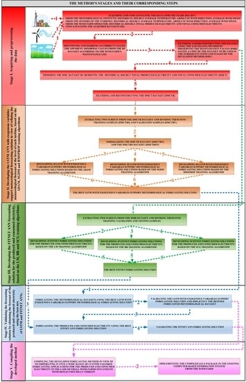
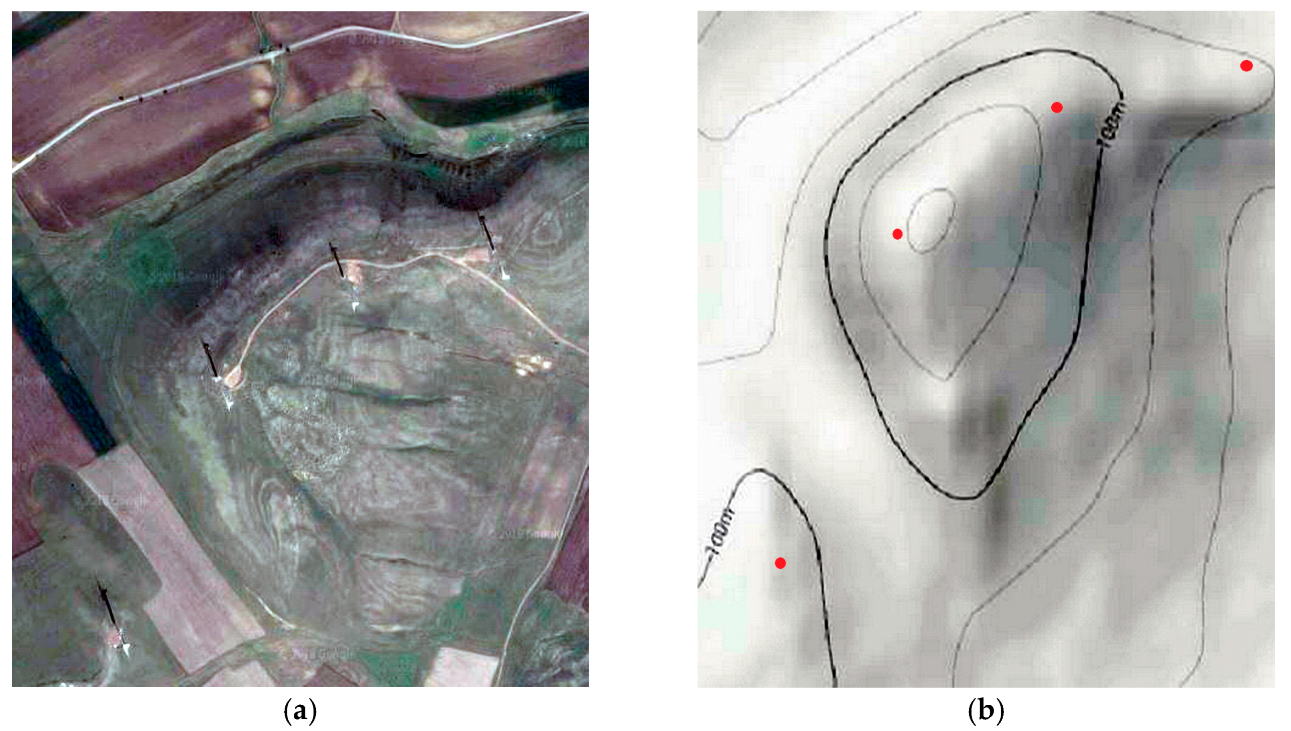
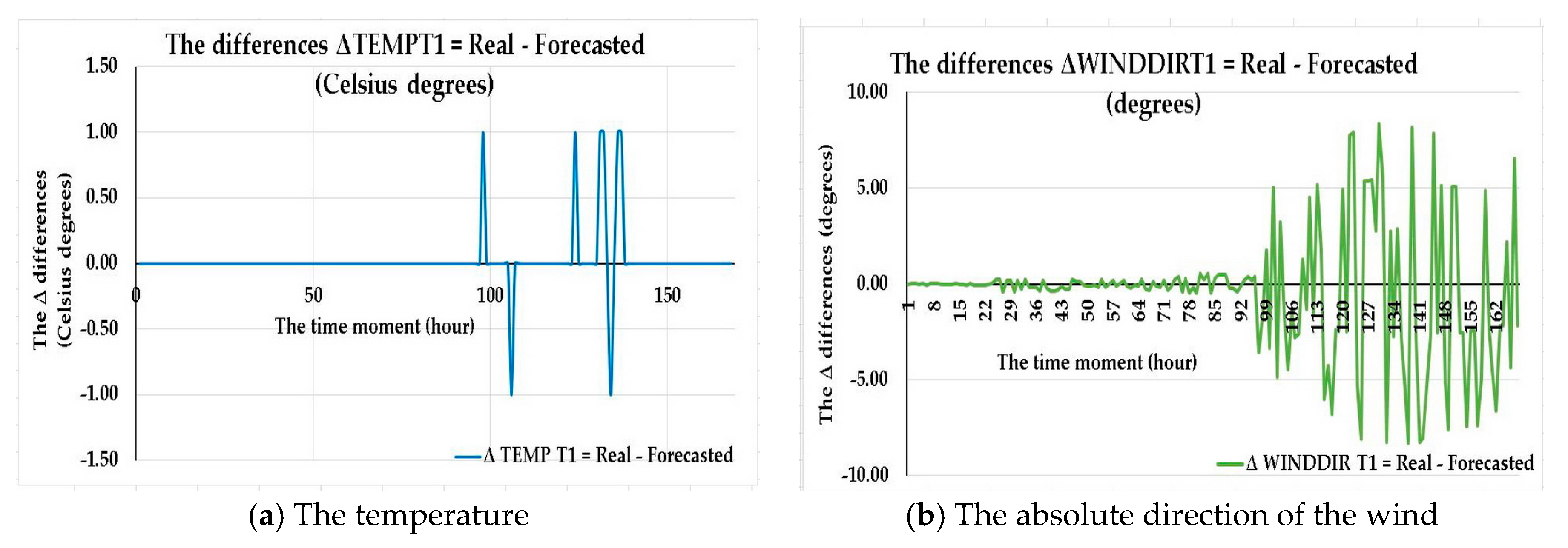