Resonant Pulsing Frequency Effect for Much Smaller Bubble Formation with Fluidic Oscillation


1
Department of Chemical and Biological Engineering, University of Sheffield, Mappin Street, Sheffield S1 3JD, UK
2
Perlemax Ltd., Kroto Innovation Centre, 318 Broad Ln, Sheffield S3 7HQ, UK
*
Author to whom correspondence should be addressed.
Energies 2018, 11(10), 2680; https://doi.org/10.3390/en11102680
Submission received: 21 July 2018
/
Revised: 10 September 2018
/
Accepted: 27 September 2018
/
Published: 9 October 2018
(This article belongs to the Special Issue Fluid Flow and Heat Transfer)
Abstract
:Microbubbles have several applications in gas-liquid contacting operations. Conventional production of microbubbles is energetically unfavourable since surface energy required to generate the bubbles is inversely proportional to the size of the bubble generated. Fluidic oscillators have demonstrated a size decrease for a system with high throughput and low energetics but the achievable bubble size is limited due to coalescence. The hypothesis of this paper is that this limitation can be overcome by modifying bubble formation dynamics mediated by oscillatory flow. Frequency and amplitude are two easily controlled factors in oscillatory flow. The bubble can be formed at the displacement phase of the frequency cycle if the amplitude is sufficient to detach the bubble. If the frequency is too low, the conventional steady flow detachment mechanism occurs instead; if the frequency is too high, the bubbles coalesce. Our hypothesis proposes the existence of a resonant mode or ‘sweet-spot’ condition, via frequency modulation and increase in amplitude, to reduce coalescence and produce smallest bubble size with no additional energy input. This condition is identified for an exemplar system showing relative size changes, and a bubble size reduction from 650 µm for steady flow, to 120 µm for oscillatory-flow, and 60 µm for resonant condition (volume average) and 250 µm for steady-flow, 15 µm for oscillatory-flow, 7 µm for the resonant condition. A 10-fold reduction in bubble size with minimal increase in associated energetics results in a substantial reduction in energy requirements for all processes involving gas-liquid operations. The reduction in the energetic footprint of this method has widespread ramifications in all gas-liquid contacting operations including but not limited to wastewater aeration, desalination, flotation separation operations, and other operations.
1. Introduction
Gas-liquid contacting operations are arguably among the most important processing operations. The oil we produce, the air, the food, the drinks (fizzy drinks, beer, and fermented beverages), chemical dyeing processes, mixing operations, wastewater aeration (WWA). and remediation, and several operations require good gas-liquid contacting [1,2,3,4]. One way to achieve such contacting is by increasing the surface area of the system corresponding to its volume. This results in an increase in surface area with respect to volume, and for a bubble, results in a slower rise velocity and a substantial increase in contact time. The major problem with smaller bubble generation is the energy required due to the large surface energy involved in generating these smaller bubbles.
Two examples where the bubble size in terms of number and volume contribution matters are dissolved/dispersed air flotation (DAF) and wastewater aeration (WWA). Both these operations are important, mandatory for any wastewater remediation, and highly energy intensive. DAF uses 70–100 µm size bubbles, generated by involving high pressure nozzles (14–15 bar (g)) [5], in order to separate systems out for remediation or further processing. Variants of this method include froth flotation such as for mineral processing−copper ore processing, effluent removal from gas processing/ petrochemical plants, paper mills, and drinking water plants. The second is WWA which accounts for nearly 0.25–0.4% of the UK’s total energy consumption [6]. This is due to the barriers to implementing high energy microbubbles and the inability to produce these in an energy efficient manner.
If smaller bubbles could be generated with less energy, it could lead to a fundamental change in gas-liquid contacting equipment design. Of particular importance to the interplay between fluid flow and heat transfer are applications of microbubbles in phase change separations, particularly vaporisation and distillation [7,8,9,10]. Experiments and models [7,10] demonstrate the layer height of liquid is extremely important, with fixed microbubble size, for determining the degree of non-equilibrium separation and the overall rate of vaporization. The highest vaporization and the greatest enrichment for 100 μm diameter microbubbles occur with a contact time of ~1 ms. Since bubble rise rate at terminal velocity is well established to depend on bubble size, hitting the optimum vaporisation rates and enrichment (joint heat and mass transfer at the microbubble interface) strongly depend on tuning the microbubble size. The purpose of this paper is to explore how microbubble size depends on the fluid dynamics of fluidic oscillator induced microbubble generation.
There are several methods to generate microbubbles such as ablative technology, ultrasound, microfluidic devices, nozzles, and other techniques, but each faces problems either due to scalability or energy input [11,12,13,14,15,16,17]. Microbubbles have been divided into several size classes and depend on the application [18]. In this paper, microbubbles are gas-liquid interfaces (bubbles) ranging from 1 µm to 1000 µm in size. Several applications have been identified for them including microalgal separation [19], wastewater clean-up [20,21], theranostics [22,23,24], algal growth [25,26,27,28], oil emulsion separation [29] and for heat and mass transfer applications (due to the vastly increased surface area to volume ratios) [30,31,32]. A major advantage is gained if a different bubble generation regime can be formulated such that it does not specifically depend on the conventional form of detachment.
The fluidic oscillator is a fluidic device that creates hybrid synthetic jets which help engender microbubbles in an economical fashion via pulsatile flow through the aerator. The adherence of the jet to the wall, due to the Coandă effect, and its subsequent detachment to the other leg due to a switch over created by a geometric cusp [33,34,35] generates the pulsatile flow. The actual mechanism of bubble formation via fluidic oscillation resulting in the back flow into the membrane due to the net positive displacement is responsible for the smaller bubble size and has been demonstrated by Tesař [35]. Zimmerman et al. [9,30,35] have shown the efficacy of the fluidic oscillator with respect to bubble size reduction via aeration.
Although introduction of the negative feedback can be achieved using both the Warren and the Spyropoulos configuration for the fluidic oscillator [36], for the experiments herein, to facilitate the use of discrete frequencies, a Spyropoulos type feedback loop has been used. This type of negative feedback has several advantages. Firstly, frictional losses are kept to a minimum and secondly, the frequency of oscillation can be easily controlled by changing the negative feedback configuration i.e., with the use of different feedback loop lengths and volumes.
The Spyropoulos loop has been adequately described in Tesař et al. [37], which introduces a negative feedback to the system and in physical form is a single loop connecting the control terminals of the fluidic oscillator shown in Figure 1 as X1 and X2. S (supply nozzle), X1 and X2 (control terminals) and Y1 and Y2 (outlets). The incoming jet enters via the supply nozzle, is amplified at the throat via a constriction of appropriate size. Control terminals aid in switching the flow due to a pressure differential formed in order to switch on outputs Y1 and Y2 at relevant frequencies. Y1 and Y2 can be connected to microporous diffusers placed in a liquid stream which result in bubble formation when oscillatory gas exits Y1 and Y2 and into the microporous spargers. Typical widths for X1 and X2 are 2–4 mm. Fluidic oscillation is a nozzle free bubble generation method which also allows generation in the laminar flow mode. This is contrasted with conventional nozzles used for microbubbles in dissolved air flotation microbubble generation or droplet generation [38].
An added advantage of using a single feedback loop over the two required for the Warren type oscillator is that there is a reduction in the degrees of freedom, which results in a simpler system to control and quantitatively understand it.
The usual method for bubble generation using fluidic oscillation is using two outlets connected to a set of bubble generating microporous membranes (spargers/aerators) placed under liquid of interest and gas entering via supply nozzle S. The entire flow can be utilised for the generation for bubbles and this results in an unvented condition for the fluidic oscillator.
Venting this jet, increases the momentum of the pulse post the fluidic oscillator as the oscillator is a flow amplifier. The flow switches from each leg, and if the momentum of the jet and therefore the pulse strength associated with the jet can be increased whilst maintaining the appropriate flow into the aerator.
Bubble formation conventionally requires the bubble to detach when the forces acting on it are balanced. According to Zimmerman et al., the proposed mechanism for bubble formation mediated by the fluidic oscillator typically takes place in the pulse cycle of the frequency switch. Therefore, technically this should lead to a bubble formed at every pulse and the throughput determined by the frequency of the oscillator. However, this does not take place as seen in the previous papers [9,30,35]. Each pulse of air is based on the frequency of oscillation. This means that higher the frequency, shorter the oscillatory pulse, and therefore in theory should lead to a smaller bubble. This has not been observed and led to one of the hypotheses proposed in this paper. The first part of the hypothesis is that the amplitude of the pulse must be high enough for detachment to occur. Post the bubble detachment, the bubbles may coalesce if the frequency is too high as they are close to each other. The frequency and amplitude of the fluidic oscillator are the two control parameters capable of producing the bubbles at the required frequencies. To increase the amplitude of the flow, higher flow rates will be used and then vented such that the actual flow into the aerator is as desired but the amplitude of the flow has increased. Different feedback conditions will be used in order to see the variations of the amplitude. Higher feedback conditions will have a higher amplitude whilst lower feedback conditions will introduce a higher friction loss and therefore lower resultant amplitude of the flow.
The second part of the hypothesis is that there is a resonant condition for the system which depends on a specific frequency which determines the bubble size. Even when the amplitude condition is met and bubbles are generated at each pulse, just increasing the frequency will not result in a smaller bubble size. At a specific frequency, there will be the presence of the resonant mode condition, where the bubbles are detached, but not too quickly so as to coalesce, and not too slowly so as to resemble a conventional steady flow bubble formation. The paper aims to explore this new regime of bubble formation and check if the hypothesis is supported with experimental evidence.
The flow has to be vented in order to generate higher amplitude of the jet and only partially diverted into the aerators used for bubble generation. This helps in two ways—it increases the effect of the oscillatory flow (by virtue of an increase in amplitude by increasing momentum of the wave) in order to observe the difference between discrete oscillatory flow conditions (frequencies) for the lab scale and minimises the bubble coalescence due to the increased momentum imparted to the newly engendered microbubble. This fluidic oscillator mediated oscillation has an amplitude and frequency dependence on the inlet flow rate to the oscillator provided that all other conditions are maintained. This proposed addition to the experiment enhances the fluidic oscillator mediated microbubble size reduction.
Several industrial applications can afford to have gas wastage for a significantly larger bubble throughput concomitant with reduced bubble size. Since air, in particular, is not that expensive with respect to the decreased energetics, this is justified by the increase in reaction surface area and the lack of maintenance requirements with the no-moving part fluidic oscillation.
Figure 2 shows the vented schematic of the fluidic oscillator with V1 and V2 acting as the vents to the system. Additional venting ensures that the appropriately controlled flow can pass through the aerator whilst maintaining the appropriate flow into oscillator in order for it to actuate the oscillation. Additionally, this increases the momentum of the jet and the amplitude of the oscillatory flow.
Conventional bubble formation depends on a host of other factors such as surface energy of the bubble engendering surface and the liquid, liquid and gas viscosity, momentum of the gas, height of liquid, pressure exerted by the system and acting upon it, and size of the bubble-engendering orifice. Fluidic devices such as the Tesař-Zimmerman fluidic oscillator generate a net positive hybrid synthetic oscillatory jet that results in a specific reduction in bubble size compared to conventional or steady flow as discussed previously.
2. Methods and Materials
2.1. Fluidic Oscillator
The fluidic oscillator is oscillated at 86 L per min (lpm) and 92 lpm (corrected for pressure and temperature) with most of the flow being vented and a frequency sweep is performed in order to support the hypothesis posited earlier. As discussed previously, vents have been introduced in order to increase the momentum of jet pulse and amplitude of oscillation whilst controlling appropriate flow into the aerator (MBD 75, Point Four Systems, Coquitlam, BC, Canada). Rotameters have been utilised to act as metered valves. The frequency of oscillation and the amplitude of the oscillation are measured using an Impress G-1000 pressure transducer (Impress Sensors and Systems, Ltd., Berkshire, UK) controlled and recorded using characterisation software developed in LabView (National Instruments, Austin, TX, USA). The pressure drop across the fluidic oscillator is 100 mbar. The total pressure drop depends on the combined pressure drop across the fluidic oscillator and aerator.
2.2. The Aerator
The proprietary Point Four Systems MBD 75 aerator produces a cloud of fine bubbles approximately 500 µm in size under steady flow. MBD 75 has ultrafine ceramic pores and a flat surface, thereby retarding bubble coalescence as compared to other types of material such as sintered glass or steel membranes. Ceramic, being inert, hydrophilic and robust, is a preferred surface for bubble generation in water.
2.3. System Set up
The system has been set up according to the schematic shown in Figure 3.
2.4. Pneumatic Set Up
Figure 3 shows the system schematic described here. The pressure regulator (Norgren, Littleton, CO, USA) controls the systemic pressure which is set at 2 bar(g)—the required pressure for the particular aerator to bubble. A different aerator would require lesser pressure. The flow controller (FTI Instruments, Sussex, UK) has been corrected for the pressure being used in the system. The air enters the system from the compressor via the pressure regulator and the flow controller regulates the global flow entering the fluidic oscillator. The fluidic oscillator is connected to two vent rotameters (F1 and F2) to act as metered valves and these are set up in order to vent appropriately and send the appropriate amount of flow into the aerator. The aerator is placed in a tank wherein the bubble size is measured using acoustic bubble spectrometry.
The frequency and amplitude of pulse from fluidic oscillator is measured simultaneously using a combination of pressure transducers and Fast Fourier Transform (FFT) code developed in LabView (cf. frequency measurement and FFT).
The aerator is kept in the centre with the hydrophones set around it as shown in Figure 4 with the set operational conditions. Bubble sizing is performed continuously and the distilled deionized (DDI) water in the tank is replaced after each reading.
The frequency is changed whilst all other conditions are kept constant and different feedback configurations are used coupled with an additional flow rate. This is an exemplar system and we are just demonstrating the ability for the system to change with different systems and the aim of this paper is to show that relative changes are possible for the system without any additional energy input. Several configurations of the Spyropoulos type fluidic oscillator being used are also able to engender the same frequency which helps observe the effect of the frequency.
2.5. Bubble Sizing Using Acoustic Bubble Spectrometry
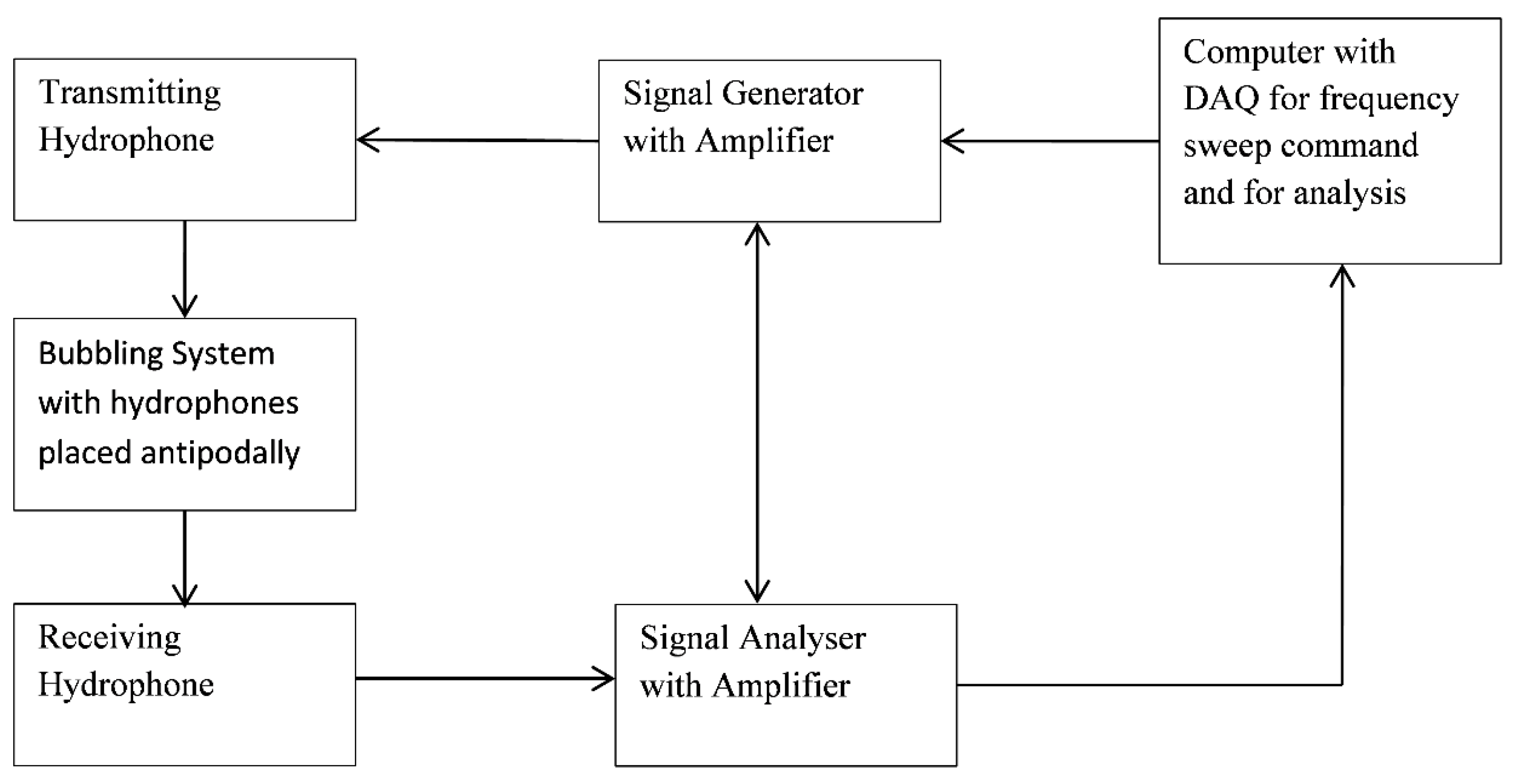
The hydrophones are placed over at a height 5 cm above the diffuser and equidistant at 15 cm. These data were repeated 7 times and performed at 2 different flow rates—86 lpm and 92 lpm (standard conditions—293.15 K and 101,325 Pa ). Twenty two frequencies were used in the study performing a frequency sweep and 3 different configurations of feedback for fluidic oscillator. Bubble sizing was performed using Acoustic Bubble Spectrometry commercially available from Dynaflow Inc.™ (Jessup, MD, USA). This has been found to be an effective method for visualising cloud bubble dynamics. The Acoustic Bubble Spectrometer (ABS) with 4 pairs of hydrophones—50, 150, 250, and 500 kHz were used in this study, with the capability to collate a size distribution from 3 µm to 600 µm in size (radius). The ABS is then set up along with an octaphonic set up and Figure 4 schematically represents the flow diagramme of the bubble visualisation set up.
Two equiresponsive hydrophones are placed antipodal to each other with the aerator bubbling in the centre i.e., bubble cloud in the centre. The data acquisition module and computer (controlled using software) send out a frequency sweep via a signal generator with amplifier into the transmitting hydrophone. The signal passes through the bubble cloud (calibrated under no bubble condition) and into the receiving hydrophone which is demodulated using an amplifier too. This is used in conjunction with the no bubble condition in order to generate a bubble size distribution.
Acoustic bubble sizing relies on the principle of bubble resonance upon frequency insonation and the resonant bubble approximation. Upon insonation by a specific frequency, a bubble starts to oscillate and this frequency is specific to the bubble by a sixth power to the radius, i.e., [39]:
Hydrophone pairs are used, with one being a transmitter and the other acting as the receiver, and each hydrophone pair has a specific resonant frequency at which it works best and a range of frequencies that it can operate reasonably. When a hydrophone insonates a bubble cloud with a specific frequency, the bubble corresponding to that size resonates and therefore oscillates, thereby attenuating the signal due to the pressure change caused by the oscillating bubble as compared to a clear/bubble-free solution. This attenuation is then measured by the receiving hydrophone and the signal is inverted in order to garner a bubble size distribution. A frequency sweep is performed at equally spaced frequencies between 5 kHz to 950 kHz, from which the bubble size distribution is compiled. Chahine et al. [40,41,42,43,44,45,46] describe the methodology underpinning ABS and the algorithm for transformation of the raw data into a bubble size distribution.
2.6. Frequency Measurement and Fast Fourier Transform
Impress G-1000 pressure transducers were used in this experiment. Fast Fourier Transforms are simple algorithms designed to convert a signal from one domain (time or space) and convert it to the frequency domain and vice versa. Figure 5 shows an exemplar waveform with the FFT. This provides a quick and easy way to determine the frequency of the oscillatory flow from a fluidic oscillator. LabView is used to acquire the signal and process it. The oscillatory pulse from a fluidic oscillator is composed of the amplitude and frequency of oscillation.
2.7. Bubble Sizing Analyses
Two factors are readily computable for the bubble size analysis obtained from the ABS- average bubble size in terms of number of bubbles and average bubble size in terms of void fraction contribution (volume contribution) of the bubble. Depending on the application, bubble sizing is usually reported using either of these two factors. Since volume contributions (due to their association with increased mass transfer/heat transfer for microbubbles) are more relevant for a majority of industrial processes, this paper discusses bubble sizes in terms of volume contributions.
Table 1 provides an exemplar for a case wherein there are three classes of bubbles—Class A—with a size of 1 μm and 600 in number, Class B with size of 100 μm and 200 in number and Class C of size 500 μm and 200 in number. This would lead to a total of 1000 bubbles. The surface area of the bubbles is calculated and so is the volume. The bubble size can be computed by either using average bubble size in terms of numbers i.e. weighted bubble size divided by total numbers, or in terms of average bubble size in terms of volume contribution i.e., weighted bubble volume divided by total bubble volume:
with:
where average bubble size in terms of number (2) volume (3) is shown, n is the total number of bubbles and ni is the bubble contribution for number (2) volume (3) of each bubble of size xi represented by Vi (4).
This also means that 1 million 1 µm bubbles would be required to occupy the same volume as a single 100 µm bubble. This brings about a massive disparity in bubble size in terms of volume contribution. However, the volume contribution would be a useful tool for estimating any transport phenomena exercise over number contribution. Generally speaking, size distributions collated from membranes are narrow and the difference in the two averages is lower. A large difference in bubble sizes is observed for a highly dispersed distribution and it is beneficial to the system to have a narrower size distribution. This exemplar demonstrates how these two values need not be the same and their dispersity results in the width of the bubble size distribution. Work by Allen [47] and Merkus [48] explain the nuances associated with particle sizing and statistical calculations performed for them in detail.
2.8. Results and Discussion
In order to prove the hypotheses, two experimental modalities were tested. Bubble sizes were measured at various frequencies and under different conditions. Bubbles were sized at 22 frequencies, for three feedback conditions (to test amplitude variations) and two higher flowrates (vented, so flow through the fluidic oscillator could be 86 lpm and 92 lpm). Bubble size for steady flow at the same conditions resulted in a bubble size of approximately 350 µm and 450 µm, respectively. This confirmed previous work performed in literature [19,30,49] that fluidic oscillation resulted in a significant decrease in bubble size when compared to conventional methods of microbubble generation.
An approximate 60% reduction in bubble size than the average bubble size estimated from oscillatory flow at other frequencies was observed for all configurations, supporting the proposed hypothesis. The variations between the amplitudes provided additional information on this new bubble formation dynamic under the resonant mode regime.
With the configuration that induced the highest negative feedback, there is a suggestion that two dips observed and this is probably due to the higher feedback introduced for oscillatory control thereby changing the effect of the system.
Figure 6 shows the length of feedback loop compared to the average bubble size at two amplitudes. This shows that although the conditions have been slightly changed, the resonant condition observed is at the same frequency as can be seen in Figure 7. The frequency of the fluidic oscillator can be changed by changing the feedback loop length. This changes the amount of feedback introduced into the system. Figure 6 shows that although the dip is at the same frequency, the actual feedback loop is different for both cases for different conditions of feedback loop lengths. This causes the slight shift in the frequency observed for the dip.
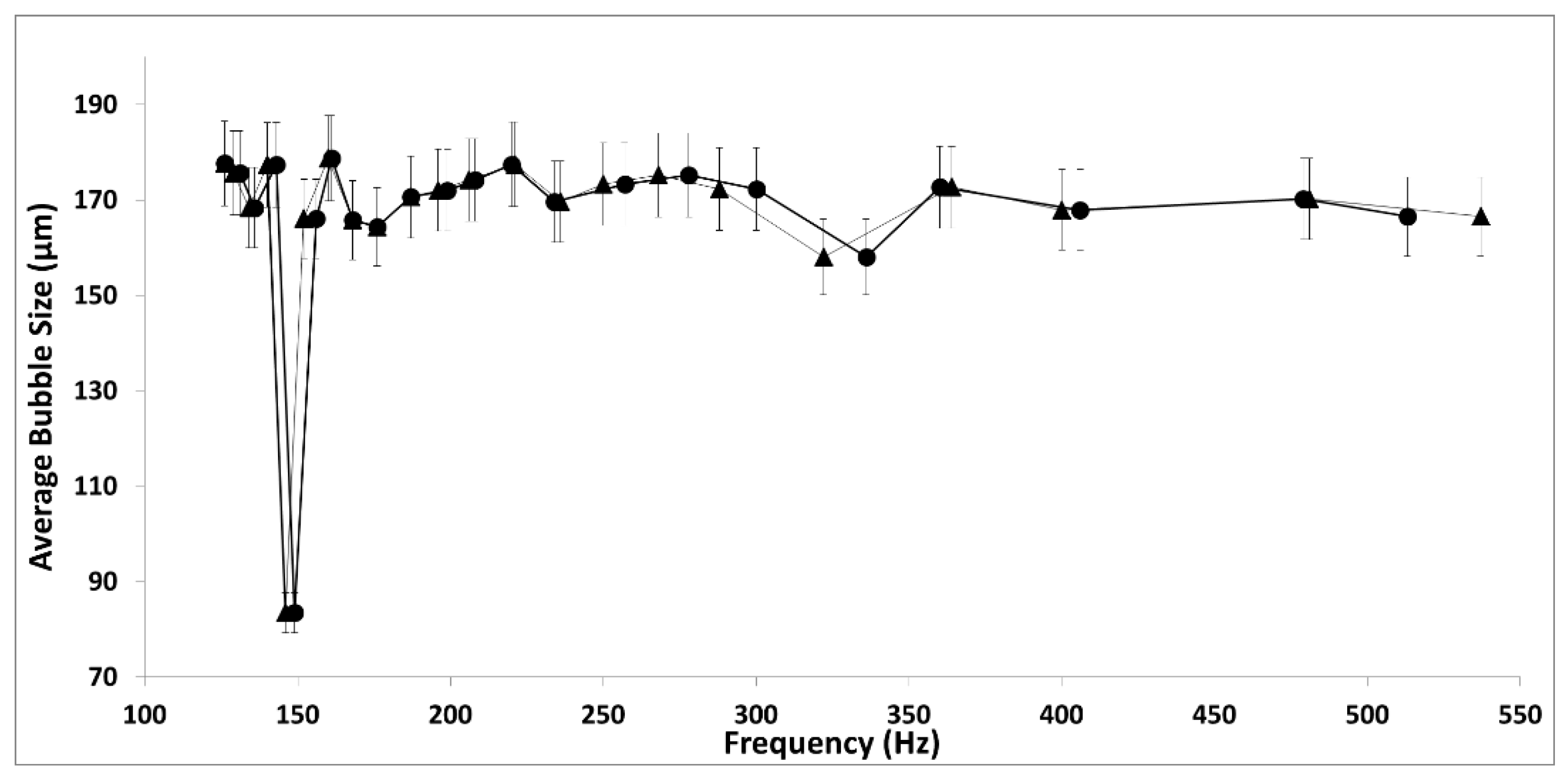
Figure 7 shows the average bubble size at different flowrates when the frequency is modulated for the smallest feedback configuration. At these two conditions, it is observed that the primary dip occurs circa 150 Hz. The dip is large and observable and there is a suggestion of another dip prior to that. This is shifted slightly for different amplitudes. This is what is seen herein. The frequency remains the same for different configurations of feedback, resulting in a change in bubble size even for different conditions.
Varying the lengths of the tube were used to introduce a change in the feedback. Figure 6 and Figure 7 show that even though the feedback loop lengths were different, the frequency change observed due to the change in flow rate with respect to feedback loop length resulted in a minimum bubbles size at the same frequency. Figure 6 and Figure 7 are plots from a reading taken for single tubing, lowest feedback configuration, at two different inlet global flow rates at 22 different frequencies. The bubble size distribution showed the dip in bubble size and the resonant mode—‘sweet spot’ was observed here. Figure 6 shows the presence of the ‘sweet spot’ at different lengths of the feedback loop. Figure 7 shows that although the feedback loop lengths were different for the different dips in bubble size, the actual frequency remained the same and was approximately 150 Hz.
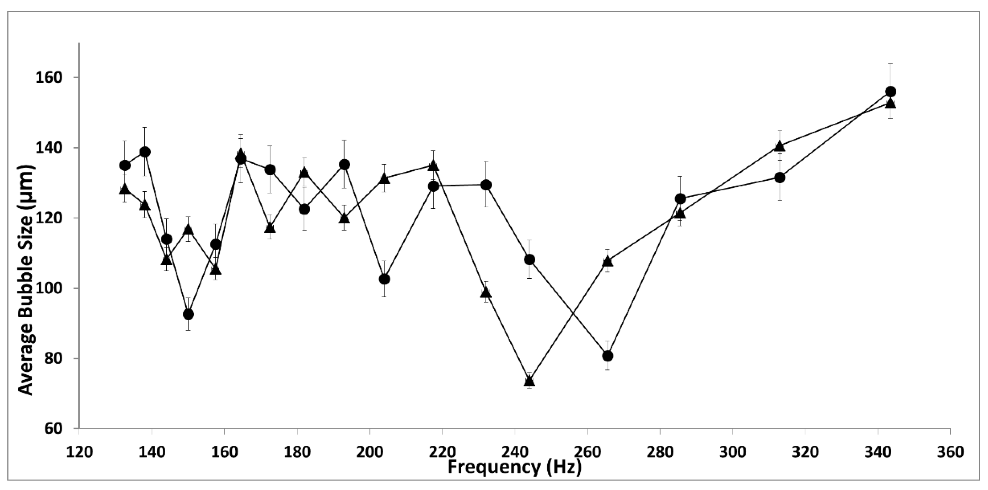
Figure 8 shows the resonant mode for the medium feedback condition. The dip is quite close to each other for this scenario. The frequency for the sweet spot is similar to the low feedback condition and is at 150 Hz. There is a significant dip observed due to potential matching of the flow rate with the frequency of the system and bubble formation.
Figure 9 shows the bubble size versus frequency at the higher feedback configuration. Resonant condition dips are observed for all three conditions as seen in Figure 7, Figure 8, Figure 9 and Figure 10.
Under higher feedback condition, i.e., 10 mm OD, the frequency is higher for the dip aside from the initial dip. This is probably due to the higher amplitude observed for the higher feedback condition which results in lesser coalescence for the system. The dip observed is still consistent with the average bubble size formed at other conditions of the resonant modes.
The presence of the resonant condition or ‘sweet spot’ was observed for the higher feedback condition. However, the magnitude of the decrease in bubble was not as significant as for the lower feedback condition (i.e., feedback loop length is constant but volume is lower) when considered in a relative manner. However, due to the greater amplitude, there is a higher frequency and several smaller bubbles being formed which results in the dampening of the ‘sweet spot’. There is another ‘sweet spot’ formed at 250 Hz.
These figures also show a skew observed in terms of frequency and flow rate, with the skew being less for the larger feedback condition than for the lower feedback configuration indicating that even the shift observed in the frequency is due to the combination of the length of the feedback tube and the flow rate and this skews the bubble size and the resonant condition.
These three conditions (amplitude variations) consistently show the resonant mode condition. The different vent flows also show the resonant mode condition and the resonant condition changes based on the variations introduced. The flow rate is an additional variable influencing the frequency [49] can be adjusted to achieve the same average bubble size. This is because the change in flow rate has a much larger impact on the frequency of the smaller feedback configuration than that of the larger one due to the difference in the frictional losses for both conditions. The dip in bubble size is observed at different feedback conditions when the global flow rate is different. However, it is the same frequency at which bubble size reduction is observed, demonstrating that the change in global flow results in no significant shift in the frequency ‘sweet spot’, ~150 Hz. Of note is that not only is a similar trend being observed at these different flow rates but there is also a clear indication of the dip in bubble size at the specific flow rate and frequency that seems to be characteristic of this newly discovered ‘sweet spot’. It is interesting to note that the extent of the dip in bubble size varies with the flow rate and therefore on the amplitude of fluidic oscillator. The ‘sweet spot’ depends on the fluidic circuit i.e., aerator, liquid, fluidic oscillator, and gas aside from incoming flow rate. Amplitude is one of the major causes for a bubble size reduction which results in higher frequencies and bubble throughput.
Figure 10 shows the amplitudes and the differences seen for the different resonant conditions and shows the resonant condition for these configurations. It is seen that there is a greater decrease in bubble size for the higher feedback condition (i.e., higher amplitude), as also observed for higher fluidic oscillator incoming flow rate. This happens at a higher frequency because of the change in the ‘sweet spot’ condition. This means that the amplitude is higher for the same condition. This results in the lowest feedback condition having the ‘largest’ bubble size for its sweet spot condition. There is a smaller difference between OD 4 mm and OD 6 mm condition due to smaller differences in the feedback introduced as compared to the OD 10 mm. This increases the condition substantially resulting in an increase in the effect observed.
2.9. Mechanism for the Resonant Mode Condition or ‘Sweet Spot’
Bubble size is directly proportional to the rise velocity and inversely proportional to the bubble wake and liquid present in the system. There are two ways that can be used to increase the amplitude to test the hypothesis we have proposed—increase it by imposing a higher feedback (i.e., 10 mm OD volume) or by increasing the flow through the fluidic oscillator (86/92 lpm). Both conditions have been used in this study and this provides several conditions to observe for fluidic oscillation mediated bubble formation. The change between the OD 4 mm and OD 6 mm is not as significant as between the two and OD 10 mm. This is due to the large feedback introduced in the system in order to cause an improved performance regime in terms of momentum of the jet as well as amplitude of the oscillatory pulse.
This results in different systems being imposed whilst keeping the rest of the system as constant as possible. The reason why different aerators were not used was because it would be difficult to compare two aerators (they can have several different properties—wettability, porosity, thickness, mesoporosity, polydispersity of orifice sizes, material of fabrication, and pressure drop across the membrane.
3. Dimensionless Analysis
The dynamics of bubbles generated in an oscillatory system can be defined by dimensionless quantities such as the Weber Number—We, Stokes Number—Sk, Strouhal Number—Sh and Reynolds Number—Re.
We is defined as the ratio of the inertia of fluid to its surface tension and determines the curvature of the bubble which means smaller the bubble greater is the curvature and higher is the surface tension and higher the We. Sk relates the bubble size to the rise velocity of the system whereas the Sh is used for oscillatory systems and for the fluidic oscillator, helps determine the frequency of bubble generation and the characteristics of the fluidic oscillator, especially the oscillatory flow and bistability.
Conjunctions occur when either of these values is unbalanced, leading to a bigger bubble size being observed. Greater unbalance leads to coalescence in the system. Tesař et al. [50] describes the case of the smallness of microbubble being limited due to coalescence:
f = oscillation frequency (Hz), L = length of feedback loop (m), V = supply nozzle bulk exit velocity (m/s), b = Constriction width (m), ρ = density (kg/m3), ƞ = viscosity (Pa.s), Dh = Hydraulic diameter (m), v = specific fluid volume (m3), w = bubble rise velocity (m/s), Db = bubble diameter (m), and σ = surface tension (N/m).
Sanada et al., [51] discussed the coalescence observed in rising bubbles and the interactions between two rising bubbles. This interaction depends on the rise velocity, (therefore size) and the rate of formation of the bubble (oscillation velocity in case of fluidic oscillator). Therefore this means that coalescence is directly related to the We, (bubble formation and size), Sk (bubble rise and size), Sh (bubble formation via oscillation and oscillatory flow) and Re (determining the momentum carried by the bubble due to the pulse). This, coupled with the resultant bubble wake and zeta potential (if any due to presence of ions/ surfactant layers on the system), defines the ultimate bubble size. This does not account for the fact that the surface of the membrane generating the bubble (involves the We and WeOscillatory since surface tension is involved) and the orifice size (dependent on Sh since it is the constriction that determines the bulk exit velocity of the orifice).
A conclusion to be drawn from this is that if there is the appropriate balance in the system, (with respect to rise velocity, frequency of bubble generation, bubble size and orifice diameter), analogous to a resonant mode of the system where these conditions are balanced just about correctly, then bubble conjunctions would be avoided leading to a significant size reduction in the bubbles. This is a substantial reduction in size by optimising the parameters of an existing system without any modifications or retrofitting. The amplitude of the pulse is also important as it increases the Sk and Sh which results in lesser conjunctions and coalescence.
• Force Balance:
Balancing the forces on the bubble being formed as seen in Figure 11.
Figure 11 shows the forces on a bubble detaching and being formed. The buoyancy force and momentum force act upwards, the cosine component of the wettability (anchoring force), drag force, surface tension act downwards. For an orifice of diameter D, density of liquid—ρL, density of gas—ρg and volume of bubble former—Vb, the following equations are obtained for the forces acting upwards:
• Bouyancy Force
resulting in:
• Momentum Force
taking downward forces into account.
• Wettability Force
where θ is the wetting angle / contact angle made by the engendering bubble and the surface and σ is the surface tension force / anchoring force/ wetting force and Do is the diameter of the orifice.
• Drag Forces
with the rise velocity denoted by ub.
• Bubble Inertial Force
where Vb is the bubble volume, ρg is the gas density, ρl is the liquid density, g is the acceleration due to gravity, Db is the bubble diameter, D is the orifice diameter, ub is the rise velocity of the bubble centre , Cd is the drag coefficient and Q is the volumetric gas flow rate.
Our hypothesis comes from the fact that the bubble formation is most dependent on frequency of the system for oscillatory flow and the amplitude associated with it. If these two are appropriate, such that the bubbles are formed at regular intervals, fast enough to have substantial size reduction (reduction of pulse length and increase in throughput) and not too fast as to coalesce, with the increase in amplitude such that the bubble will cut off instantaneously and not coalesce. Balancing these forces together would result in pinch off. Compensation must be provided for the bubble rise and pinch off due to the oscillatory flow. The force balance turns out to be complicated due to the oscillatory waves and the hybrid synthetic jet engendered by the oscillator, resulting in a highly non-linear system.
• Prediction of Bubble Size at Resonant Frequency (Volume-based Bubble Size)
It is seen in Tesař et al. [53] that the bubble rise is dominated by the coalescence and each individual coalescing bubble leads to an increased probability for another staged coalescence which leads to largeness in bubble size as compared to the orifice. Once two bubbles merge together, due to the increase in size and the change in the surface energy as well as the energy associated with the ascent, it is easier for the other bubble to catch up with it. This is better explained by the concept of bubble wake. Each bubble creates a wake (region of lower pressure) upon being created and this allows other bubbles to catch up, coalesce and result in larger bubbles.
Therefore, the smaller the bubble that is created will result in a smaller wake. However, it is easier for the small bubble to be affected by a wake of another bubble (especially a larger one—which is why a smaller bubble generated after a larger one usually results in coalescence.
The active diffusing area of the aerator is 0.15 × 0.03 m2. The bubble flux recorded by the acoustic bubble spectrometry is based on the capture rate or acquisition rate that is set for the system at 200 ms. The 200 ms ensures that the flow in the system is captured at a fixed rate and this results in a delimiting information due to the resultant lower acquisition observed. The capture results in determining the flow to be 0.5 lpm. Using these results, a size of 74 µm approximately is observed. This is thus the minimum size achieved for this. Taking this value and placing it in the equations (10–16) results in the bubble formation force, and taking a frequency of 150 Hz as the bubbling frequency, and the bubble flux from the ABS (120,000) it results in a pulse requirement of 0.007 bar to detach the bubble. This has been achieved by the oscillator as observed in Figure 5 and therefore explains the sweet spot possibility for these conditions of resonance.
Figure 5 shows that the amplitude of the pulse is approximately 0.2 V, which is equivalent to 0.02 bar. This is roughly twice the required pulse strength for the bubble formation and this is why the bubble is detached at the frequency. Judging by that, the frequency band is slightly wide due to the lack of coalescence at this point.
The amplitude of the pulse reduces as the frequency increases for the same flow resulting in intermittent pinch off (since the amplitude is important for imparting sufficient force for bubble detachment). Lower frequency has a larger amplitude but the rate of generation is not fast enough. Additionally as can be seen in Tesař ([34,50]), the coalescence perpetuates the higher rise velocity of the larger bubble. This results in larger bubbles for the non-resonant conditions at lower frequencies. Therefore, the resonant condition or ‘sweet spot’ is possibly the only condition where the amplitude, frequency, and size are balanced so as not to have bubble coalescence.
There is greater amplitude for the higher feedback condition which results in the ‘sweet spot’ occurs at a higher frequency (250 Hz). This is what results in the larger increase in the number of bubbles throughput.
• Prediction of Bubble Size at Resonant Frequency (Number of Bubbles-Based Bubble Size)
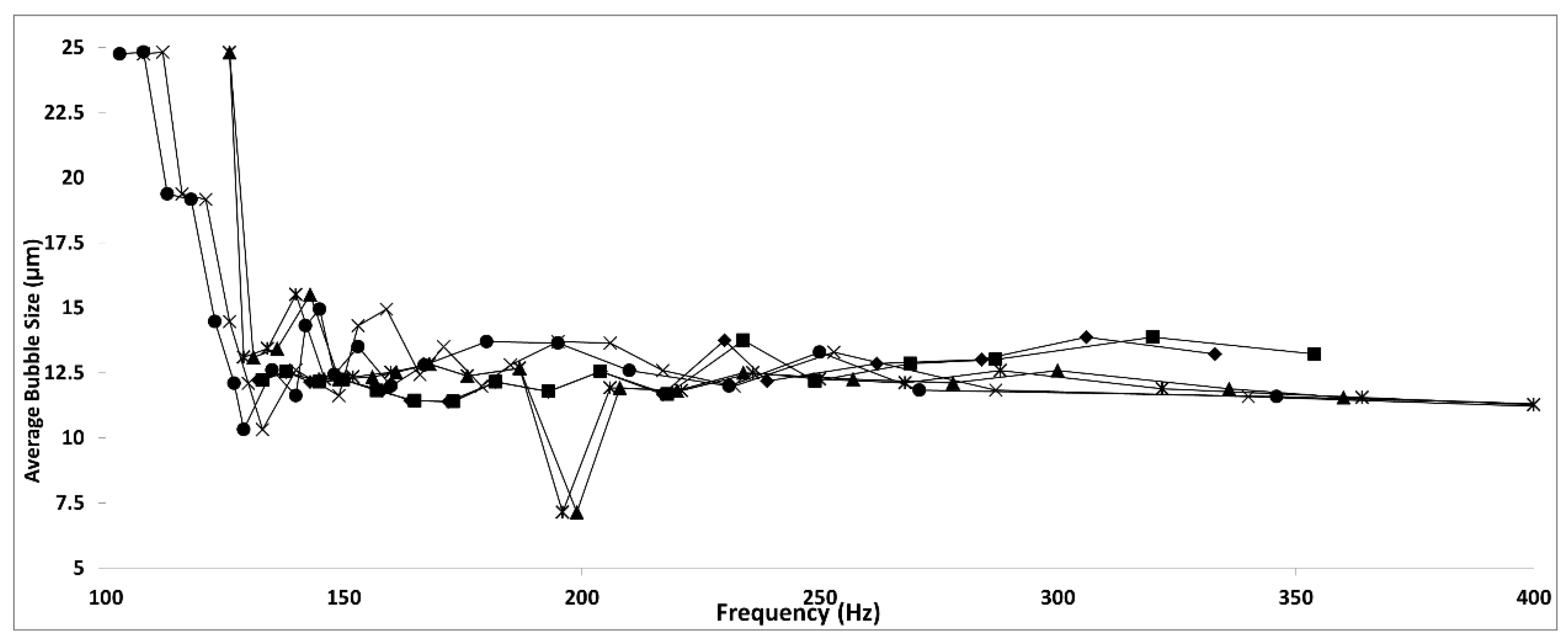
This paper has placed a lot of emphasis on bubble size suitable for transport phenomena but for finding out what the actual bubble size is, when compared to those that have been reported previously, such as Hanotu et al. [19], the size distribution based on number of bubbles calculation—NAv, provides a better idea for those applications concerned with size of the bubbles (flotation/DAF for example) in Figure 12.
This brings down the average bubble size reduction producing about 7 µm size bubbles in terms of average size distribution which makes it suitable for generating the bubbles for flotation studies. The ‘sweet spot’ changes to 200 Hz. This is because the size distribution changes due to the change in flow dynamics. The flow results in this size change as the effect of the number of bubbles cannot be discounted just as the volume average bubble size depends on the dispersity of the size distribution.
An example is provided herewith: The outlet flow of the diffuser measured at 0.1 lpm (1.67 × 10⁻⁶ m3/s) for which, when corrected for the 200 ms acquisition rate of the ABS is Q = 3.33 × 10⁻⁷ m3/200 ms. N = No of Bubbles— Approximating total number of bubbles as 120,000 as an average measured from the readings, assuming that the distribution is narrow (for the purposes of a general understanding).
Assuming that since bubble pinch-off force (by using Equations (10)–(16)) results in 0.007 bar, and the pulse of the oscillator is an average of 0.02 bar, it exceeds the force required for bubble pinch-off (cf. Figure 5). As seen from the FFT of the pulse for the oscillator, the pulse strength is at 0.02 bar per pulse which ensures that there is sufficient momentum and amplitude to generate the bubbles and ensure that the bubble detaches at each oscillatory pulse, so it is an accurate assumption providing no coalescence takes place. This is why the sweet spot is likely at 200 Hz as for the same momentum the force of the bubble pinch-off seems to be at the appropriate level. Figure 5 is shown herein for reference. This has been done in order to reduce the bubble size by matching the bubble formation characteristics to achieve the lowest possible bubble size and by increasing the amplitude of the oscillation in order to impart momentum to the jet and therefore the bubble so that it has a higher rise velocity. This reduces the bubble coalescence when the appropriate conditions are met. Too slow, and the bubble does not detach quickly enough and therefore coalesces, too fast, and the bubble cannot detach due to reduced amplitude and pinch-off. At the right frequency and amplitude, what we term—resonant condition or ‘sweet spot’, one can detach the bubble at the smallest possible size for that system and it is significantly smaller than what was originally possible via conventional steady flow. This is achieved for the frequency at 200 Hz. Since f = 200 Hz means that it is per second, for 200 ms, the equivalent frequency to be considered would be 40 Hz.
Using the A = diffusing area (0.15 × 0.03 m2), and assuming that all the flow forms a bubble (there are no leaks and the bubble sizes are small enough to form bubbles rather than slugs:
which results in DB i.e., (2r) = 6.8 µm for 200 Hz.
This is in close agreement to the size obtained in the system. Depending on changes introduced to the system, these values will change. Whilst these values will change depending on the system, the work supports the presence of the resonant bubbling condition that can occur in any oscillatory flow mediated bubble generating system.
Figure 13 shows the calculations for a sweep for bubble formation via frequencies juxtaposed with the size for the bubbles that would be formed. There is an extension but this is likely due to the fact that at lower frequencies, steady bubble formation dominates as it is results in faster bubble pinch-off.
As discussed earlier, 0.25–0.4% of the U.K.’s energy use is utilised for WWA operations. This is not discussed earlier These energy requirements could be substantially reduced by bubble size reduction. The 10 fold size reduction would provide a significant increase in the transport phenomena associated with the bubbles. The cost of adding the fluidic oscillator is based on the pressure drop of the oscillator, which for an industrial plant would typically be about 400 mbar for a large scale system. The cost of frequency modulation in terms of energy is negligible. This is also applicable for several other applications and remediation steps including aeration of waste streams, oxidation of volatiles, advanced oxidation processes, and other treatment techniques. Several other processes exist where gas-liquid operations are involved and bubble sizes are required to be small.
4. Conclusions
This paper reports several scientific results. One of the major ones is the exploration of a new regime for bubble generation mediated by oscillatory flow which reduces coalescence and results in the smallest bubble formation for a given system (number averaged or volume averaged) at specific conditions of detachment with no additional energy.
The ability to generate substantially smaller bubbles, useful for several applications, by simply engineering the conditions for bubble formation under oscillatory flow such that the frequency and amplitude are maintained is a shift in understanding for bubble formation dynamics. Whilst oscillatory flow results in bubble size reduction over the gamut of frequencies, at a particular frequency, specific to a particular set up (but valid for other set ups as seen with different configurations), a substantial reduction in bubble size (≈60%) is observed. It has been hypothesised that tuning of all the different parameters controlling bubble formation will result in a smaller overall bubbles size, presumably by the combined effect of more efficient pinch off and reduced coalescence. This has resulted in a large size reduction from a typical bubble size distribution produced in a system. Conventional bubble generation would have produced bubbles of sizes: 650 µm (volume averaged) and 250 µm (number averaged), whereas the fluidic oscillator would result in an average size of 120 µm (volume averaged) and 14 µm (number averaged), and the sweet spot would result in 60 µm (volume averaged) and 7 µm (number averaged).
The addition of the fluidic oscillator reduces the bubble size to a certain extent but coalescence prevents the size being smaller than a certain range. This adds an additional pressure drop across the system by 20–150 mbar in the system (system dependent) which is insignificant compared to the actual savings in terms of surface energy. A further reduction of bubble size is achieved, without any additional cost to the system, which then brings about a step change in any gas liquid operation and overcomes any of the limitations that had been posed earlier for using microbubbles for mass transfer in gas-liquid operations. A 60% reduction in bubble size from what was already a reduced bubble size, resulting in a 10-fold reduction in bubble size with suitable tuning and adding a pressure drop of 150 mbar maximum, is paradigm shifting and has the potential to change the processing industry.
An example can be seen in DAF, which has been discussed at the start. In order to achieve a 70–100 µm bubble size (number averaged), 12–14 bar of pressure is used to generate the flux and throughput required. We can achieve a 10-fold reduction for this size (7 µm) with a tuned frequency, fluidic oscillator, and aerator totalling 2.15 bar(g) total pressure which means that the energetics involved in order to get 10 times larger size bubbles will result in substantial reduction. A simplistic approach will be to relate energy with pressure as a proxy and the energetics for a specific process can be taken into account. The fact the frequency modulation for a bistable diverter valve (the fluidic oscillator) does not require any additional energy input, but results in a 60% reduction in bubble size (increase in associated transport phenomena) [9,11,29], and is a 10-fold reduction in bubble size (100–fold increase in interfacial area) by using this tuned oscillator as opposed to a conventional steady flow system. The substantial energy saving and increase in transfer efficiencies for any gas-liquid operation involved results in widespread ramifications. This is not limited to only bistable diverters but all oscillatory flow systems as it is actually dependent on oscillatory flow and the control of frequency and amplitude as opposed to using a specific system.
These wider implications are not only limited to DAF, but for all operations that can be thought of as gas-liquid contacting or processing including aeration, gas-liquid contacting operations which constitute a large proportion of industrial processes, biochemical reactors, fermenters, remediation processes, digesters, incubators, bioreactors, and others.
Author Contributions
W.B.Z. and P.D.D. jointly proposed the central hypothesis. P.D.D. augmented the hypothesis with the inclusion of higher amplitude by artificial venting, created the experimental design and setup, and conducted the first three experiments and the design for the analysis, hence is the principal author. Y.R. provided the individual bias removal, substantial experimental work via repeats (5 in total), equation input, and collated the data for analysis. M.J.H. and W.B.Z. provided organisational and logistical support and compositional critique.
Funding
This research was funded by EPSRC grant number [EP/K001329/(1)] and part of the IUK Energy Catalyst, IB Catalyst programmes as well as the FP7 R3 water programme.
Acknowledgments
This work was carried out as part of the “4CU” programme grant, aimed at sustainable conversion of carbon dioxide into fuels, led by The University of Sheffield and carried out in collaboration with The University of Manchester, Queens University Belfast and University College London. The authors acknowledge gratefully the Engineering and Physical Sciences Research Council (EPSRC) for supporting this work financially (Grant no. EP/K001329/1). M.J.H. and P.D.D. would like to thank R3Water FP7 grant. W.B.Z. and P.D.D. would like to thank IUK IBCatalyst and Energy Catalyst award. P.D.D. would like to thank Professor Ray Allen for discussions, Audrey YY Tan for bias studies and GK for inspiration.
Conflicts of Interest
The authors declare no conflict of interest.
References
- Bird, R.B.; Stewart, W.E.; Lightfoot, E.N. Transport Phenomena; Wiley: Hoboken, NJ, USA, 2007. [Google Scholar]
- Incropera, F.P.; Lavine, A.S.; Bergman, T.L.; DeWitt, D.P. Fundamentals of Heat and Mass Transfer; Wiley: Hoboken, NJ, USA, 2007. [Google Scholar]
- Green, D.; Perry, R. Perry’s Chemical Engineers’ Handbook, 8th ed.; McGraw-Hill Education: New York, NY, USA, 2007. [Google Scholar]
- Treybal, R.E. Mass-Transfer Operations; McGraw-Hill Education: New York, NY, USA, 1980. [Google Scholar]
- Tesař, V. What can be done with microbubbles generated by a fluidic oscillator? (survey). EPJ Web Conf. 2017, 143. [Google Scholar] [CrossRef]
- Metcalf, E.I.; Tchobanoglous, G.; Burton, F.; Stensel, H.D. Wastewater Engineering: Treatment and Reuse; McGraw-Hill Education: New York, NY, USA, 2002. [Google Scholar]
- Abdulrazzaq, N.; Al-Sabbagh, B.; Rees, J.M.; Zimmerman, W.B. Purification of Bioethanol Using Microbubbles Generated by Fluidic Oscillation: A Dynamical Evaporation Model. Ind. Eng. Chem. Res. 2016, 55, 12909–12918. [Google Scholar] [CrossRef]
- Abdulrazzaq, N.; Al-Sabbagh, B.; Rees, J.M.; Zimmerman, W.B. Separation of zeotropic mixtures using air microbubbles generated by fluidic oscillation. AIChE J. 2015, 62, 1192–1199. [Google Scholar] [CrossRef]
- Al-Yaqoobi, A.; Zimmerman, W.B. Microbubble distillation studies of a binary mixture. In USES—University of Sheffield Engineering Symposium 2014; The University of Sheffield: Sheffield, UK, 2014. [Google Scholar]
- Zimmerman, W.B.; Al-Mashhadani, M.K.H.; Bandulasena, H.C.H. Evaporation dynamics of microbubbles. Chem. Eng. Sci. 2013, 101, 865–877. [Google Scholar] [CrossRef] [Green Version]
- Fiabane, J.; Prentice, P.; Pancholi, K. High Yielding Microbubble Production Method. BioMed Res. Int. 2016, 3572827. [Google Scholar] [CrossRef] [PubMed]
- Kantarci, N.; Borak, F.; Ulgen, K.O. Bubble column reactors. Process Biochem. 2005, 40, 2263–2283. [Google Scholar] [CrossRef]
- Tesař, V. What can be done with microbubbles generated by a fluidic oscillator? (survey). EPJ Web Conf. 2017, 143. [Google Scholar] [CrossRef]
- Makuta, T.; Takemura, F.; Hihara, E.; Matsumoto, Y.; Shoji, M. Generation of micro gas bubbles of uniform diameter in an ultrasonic field. J. Fluid Mech. 2006, 548, 113–131. [Google Scholar] [CrossRef]
- Shirota, M.; Sanada, T.; Sato, A.; Watanabe, M. Formation of a submillimeter bubble from an orifice using pulsed acoustic pressure waves in gas phase. Phys. Fluids 2008, 20. [Google Scholar] [CrossRef]
- Stride, E.; Edirisinghe, M. Novel microbubble preparation technologies. Soft Matter 2008, 4, 2350–2359. [Google Scholar] [CrossRef]
- Zimmerman, W.B.; Tesař, V.; Bandulasena, H.C.H. Towards energy efficient nanobubble generation with fluidic oscillation. Curr. Opin. Colloid Interface Sci. 2011, 16, 350–356. [Google Scholar] [CrossRef]
- Parmar, R.; Majumder, S.K. Microbubble generation and microbubble-aided transport process intensification—A state-of-the-art report. Chem. Eng. Process. Process Intensif. 2013, 64, 79–97. [Google Scholar] [CrossRef]
- Hanotu, J.; Bandulasena, H.C.; Zimmerman, W.B. Microflotation performance for algal separation. Biotechnol. Bioeng. 2012, 109, 1663–1673. [Google Scholar] [CrossRef] [PubMed] [Green Version]
- Agarwal, A.; Ng, W.J.; Liu, Y. Principle and applications of microbubble and nanobubble technology for water treatment. Chemosphere 2011, 84, 1175–1180. [Google Scholar] [CrossRef] [PubMed]
- Rehman, F.; Medley, G.; Bandalusena, H.C.H.; Zimmerman, W.B. Fluidic oscillator-mediated microbubble generation to provide cost effective mass transfer and mixing efficiency to the wastewater treatment plants. Environ. Res. 2015, 137, 32–39. [Google Scholar] [CrossRef] [PubMed]
- Mulvana, H.; Eckersley, R.J.; Tang, M.X.; Pankhurst, Q.; Stride, E. Theoretical and experimental characterisation of magnetic microbubbles. Ultrasound Med. Biol. 2012, 38, 864–875. [Google Scholar] [CrossRef] [PubMed]
- Lukianova-Hleb, E.Y.; Hanna, E.Y.; Hafner, J.H.; Lapotko, D.O. Tunable plasmonic nanobubbles for cell theranostics. Nanotechnolohy 2010, 21. [Google Scholar] [CrossRef] [PubMed]
- Cai, X. Applications of Magnetic Microbubbles for Theranostics. Theranostics 2012, 2, 103–112. [Google Scholar] [CrossRef] [PubMed] [Green Version]
- Zimmerman, W.B.; Hewakandamby, B.N.; Tesař, V.; Bandulasena, H.C.H.; Omotowa, O.A. Design of an airlift loop bioreactor and pilot scales studies with fluidic oscillator induced microbubbles for growth of a microalgae Dunaliella salina. Appl. Energy 2011, 88, 3357–3369. [Google Scholar] [CrossRef] [Green Version]
- Zimmerman, W.B.; Hewakandamby, B.N.; Tesař, V.; Bandulasena, H.C.H.; Omotowa, O.A. On the design and simulation of an airlift loop bioreactor with microbubble generation by fluidic oscillation. Int. Sugar J. 2010, 112, 90–103. [Google Scholar] [CrossRef]
- Ying, K.; Gilmour, D.J.; Shi, Y.; Zimmerman, W.B. Growth Enhancement of Dunaliella salina by Microbubble Induced Airlift Loop Bioreactor (ALB)—The Relation Between Mass Transfer and Growth Rate. J. Biomater. Nanobiotechnol. 2013, 4, 1–9. [Google Scholar] [CrossRef]
- Ying, K.; AlMashhadani, K.H.; Hanotu, J.O.; Gilmour, D.J.; Zimmerman, W.B. Enhanced Mass Transfer in Microbubble Driven Airlift Bioreactor for Microalgal Culture. Engineering 2013, 5, 735–743. [Google Scholar] [CrossRef]
- Hanotu, J.; Bandulasena, H.C.H.; Chiu, T.Y.; Zimmerman, W.B. Oil emulsion separation with fluidic oscillator generated microbubbles. Int. J. Multiph. Flow 2013, 56, 119–125. [Google Scholar] [CrossRef]
- Zimmerman, W.B.; Tesař, V.; Butler, S.; Bandulesena, H.C.H. Microbubble Generation. Recent Pat. Eng. 2008, 2. [Google Scholar] [CrossRef]
- Zimmerman, W.B.; Hewakandamby, B.N.; Tesař, V.; Bandulasena, H.C.H.; Omotowa, O.A. On the design and simulation of an airlift loop bioreactor with microbubble generation by fluidic oscillation. Food Bioprod. Process. 2009, 87, 215–227. [Google Scholar] [CrossRef] [Green Version]
- Tesař, V. Pressure-Driven Microfluidics; Artech House: Norwood, UK, 2007. [Google Scholar]
- Tesař, V.; Bandalusena, H. Bistable diverter valve in microfluidics. Exp. Fluids 2011, 50, 1225–1233. [Google Scholar] [CrossRef]
- Tesař, V. Mechanisms of fluidic microbubble generation part Ii: Suppressing the conjunctions. Chem. Eng. Sci. 2014. [Google Scholar] [CrossRef]
- Zimmerman, W.B.; Tesař, V.; Bandulasena, H.C.H. Efficiency of an Aerator Driven by Fluidic Oscillation. Part I: Laboratory Bench Scale Studies; The University of Sheffield: Sheffield, UK, 2010. [Google Scholar]
- Warren, R.W. Negative Feedback Oscillator. U.S. Patent 3,158,166, August 1962. [Google Scholar]
- Tesař, V. Microbubble generation by fluidics. part I: Development of the oscillator. In Proceedings of the Fluid Dynamics 2012, Prague, Czech Republic, 24–26 October 2012. [Google Scholar]
- Kooij, S.; Sijs, R.; Denn, M.M.; Villermaux, E.; Bonn, D. What determines the drop size in sprays? Phys. Review X 2018, 8. [Google Scholar] [CrossRef]
- Leighton, T.G. The Acoustic Bubble; Academic Press: Cambridge, MA, USA, 1994. [Google Scholar]
- Chahine, G.L. Numerical Simulation of Bubble Flow Interactions. In Cavitation: Turbo-machinery and Medical Applications-WIMRC FORUM 2008; Warwick University: Coventry, UK, 2008. [Google Scholar]
- Chahine, G.L.; Duraiswami, R.; Frederick, G. Detection Of Air Bubbles In Hp Ink Using Dynaflow’s Acoustic Bubble Spectrometer (Abs) Technology; Hewlett Packard: Palo Alto, CA, USA, 1998. [Google Scholar]
- Chahine, G.L.; Gumerov, N.A. An inverse method for the acoustic detection, localization and determination of the shape evolution of a bubble. Inverse Probl. 2000, 16, 1–20. [Google Scholar]
- Duraiswami, R.; Prabhukumar, S.; Chahine, G.L. Bubble counting using an inverse acoustic scattering method. J. Acoust. Soc. Am. 1998, 104, 2699–2717. [Google Scholar] [CrossRef]
- Chahine, G.L.; Kalamuck, M.K.; Cheng, J.Y.; Frederick, G.S. Validation of Bubble Distribution Measurements of the ABS with High Speed Video Photography. In Proceedings of the CAV 2001: Fourth International Symposium on Cavitation, Pasadena, CA, USA, 20–23 June 2001. [Google Scholar]
- Tanguay, M.; Chahine, G.L. Acoustic Measurements of Bubbles in Biological Tissue. In Cavitation: Turbo-machinery and Medical Applications; Warwick University: London, UK, 2008. [Google Scholar]
- Wu, X.-J.; Chahine, G.L. Development of an acoustic instrument for bubble size distribution measurement. J. Hydrodyn. Ser. B 2010, 22, 330–336. [Google Scholar] [CrossRef]
- Allen, T. Particle Size Measurement: Volume 1: Powder Sampling and Particle Size Measurement; Springer: New York, NY, USA, 1996. [Google Scholar]
- Merkus, H.G. Particle Size Measurements: Fundamentals, Practice, Quality; Springer: New York, NY, USA, 2009. [Google Scholar]
- Tesař, V. Microbubble smallness limited by conjunctions. Chem. Eng. J. 2013, 231, 526–536. [Google Scholar] [CrossRef]
- Sanada, T.; Sato, A.; Shirota, M.; Watanabe, M. Motion and coalescence of a pair of bubbles rising side by side. Chem. Eng. Sci. 2009, 64, 2659–2671. [Google Scholar] [CrossRef] [Green Version]
- Pinczewski, W.V. The formation and growth of bubbles at a submerged orifice. Chem. Eng. Sci. 1981, 36, 405–411. [Google Scholar] [CrossRef]
- Tesař, V. Shape Oscillation of Microbubbles. Chem. Eng. J. 2013, 235, 368–378. [Google Scholar] [CrossRef]
- Tesař, V.; Hung, C.-H.; Zimmerman, W.B. No-moving-part hybrid-synthetic jet actuator. Sens. Actuators A Phys. 2006, 125, 159–169. [Google Scholar] [CrossRef] [Green Version]
Figure 1.
The Spyropoulos loop configuration for the fluidic oscillator, reproduced with permission [37]. S is the supply nozzle where gas enters, X1 and X2 are the control terminals where gas switches, Y1 and Y2 are the outlets where microporous spargers can be connected with oscillatory gas output. These spargers are placed in liquid and generate bubbles.

Figure 2.
Vented Fluidic Oscillator (adapted from [37]) S is the supply nozzle where gas enters, X1 and X2 are the control terminals where gas switches , Y1 and Y2 are the outlets where microporous spargers can be connected with oscillatory gas output. These spargers are placed in liquid and generate bubbles, V1 and V2 (vents).

Figure 3.
Schematic of the setup.

Figure 4.
Information flow diagram of the Acoustic Bubble Spectrometer (ABS) and the hydrophone set up.
Figure 4.
Information flow diagram of the Acoustic Bubble Spectrometer (ABS) and the hydrophone set up.

Figure 5.
An exemple of a raw waveform from a fluidic oscillator (a) and its translation in frequency domain post FFT (b). Aliasing effects of FFT are mitigated by having a high acquisition rate (512 kHz with 512 k samples acquisition window).
Figure 5.
An exemple of a raw waveform from a fluidic oscillator (a) and its translation in frequency domain post FFT (b). Aliasing effects of FFT are mitigated by having a high acquisition rate (512 kHz with 512 k samples acquisition window).

Figure 6.
Feedback length vs. average bubble size ( ![Energies 11 02680 i001]() —92 lpm OD4 mm,
—92 lpm OD4 mm, ![Energies 11 02680 i002]() —0 86 lpm OD 4 mm).
—0 86 lpm OD 4 mm).
 —92 lpm OD4 mm,
  —0 86 lpm OD 4 mm).
Figure 7.
Frequency vs. average bubble size at different flow rates ( ![Energies 11 02680 i001]() —92 lpm OD4 mm,
—92 lpm OD4 mm, ![Energies 11 02680 i002]() —86 lpm OD 4 mm).
—86 lpm OD 4 mm).
—92 lpm OD4 mm, —86 lpm OD 4 mm).
Figure 7.
Frequency vs. average bubble size at different flow rates ( ![Energies 11 02680 i001]() —92 lpm OD4 mm,
—92 lpm OD4 mm, ![Energies 11 02680 i002]() —86 lpm OD 4 mm).
—86 lpm OD 4 mm).
—92 lpm OD4 mm, —86 lpm OD 4 mm).
Figure 8.
Frequency for bubble size—resonant mode observed—medium feedback condition—( ![Energies 11 02680 i001]() —92 lpm OD 6 mm,
—92 lpm OD 6 mm, ![Energies 11 02680 i002]() —86 lpm OD 6 mm).
—86 lpm OD 6 mm).
—92 lpm OD 6 mm, —86 lpm OD 6 mm).
Figure 8.
Frequency for bubble size—resonant mode observed—medium feedback condition—( ![Energies 11 02680 i001]() —92 lpm OD 6 mm,
—92 lpm OD 6 mm, ![Energies 11 02680 i002]() —86 lpm OD 6 mm).
—86 lpm OD 6 mm).
—92 lpm OD 6 mm, —86 lpm OD 6 mm).
Figure 9.
Bubble Size vs. frequency for two flow rates (higher feedback configuration) ( ![Energies 11 02680 i001]() —92 lpm OD 10mm,
—92 lpm OD 10mm, ![Energies 11 02680 i002]() —86 lpm OD 10 mm).
—86 lpm OD 10 mm).
—92 lpm OD 10mm, —86 lpm OD 10 mm).
Figure 9.
Bubble Size vs. frequency for two flow rates (higher feedback configuration) ( ![Energies 11 02680 i001]() —92 lpm OD 10mm,
—92 lpm OD 10mm, ![Energies 11 02680 i002]() —86 lpm OD 10 mm).
—86 lpm OD 10 mm).
—92 lpm OD 10mm, —86 lpm OD 10 mm).
Figure 10.
Comparison between amplitudes for the resonant conditions or ‘sweet spot’ ( ![Energies 11 02680 i003]() —OD 4 mm,
—OD 4 mm, ![Energies 11 02680 i001]() —OD 6 mm ,
—OD 6 mm , ![Energies 11 02680 i002]() —OD 10 mm).
—OD 10 mm).
 —OD 4 mm, —OD 6 mm , —OD 10 mm).
Figure 10.
Comparison between amplitudes for the resonant conditions or ‘sweet spot’ ( ![Energies 11 02680 i003]() —OD 4 mm,
—OD 4 mm, ![Energies 11 02680 i001]() —OD 6 mm ,
—OD 6 mm , ![Energies 11 02680 i002]() —OD 10 mm).
—OD 10 mm).
—OD 4 mm, —OD 6 mm , —OD 10 mm).
Figure 11.
Bubble forces resolved (adapted from [52]).
Figure 11.
Bubble forces resolved (adapted from [52]).

Figure 12.
This is an example of the sweet spot for the average bubble size when one considers number of bubbles as opposed to the volume fraction of bubbles. The sweet spot changes slightly but there is still a dip observed at the higher frequencies ( ![Energies 11 02680 i004]() —OD 10 mm (92 lpm),
—OD 10 mm (92 lpm), ![Energies 11 02680 i002]() —OD 6 mm (92 lpm),
—OD 6 mm (92 lpm), ![Energies 11 02680 i005]() —OD 4 mm (92 lpm),
—OD 4 mm (92 lpm), ![Energies 11 02680 i003]() —OD 10 mm (86 lpm),
—OD 10 mm (86 lpm), ![Energies 11 02680 i006]() —OD 6 mm (86 lpm),
—OD 6 mm (86 lpm), ![Energies 11 02680 i001]() —OD 4 mm (86 lpm)).
—OD 4 mm (86 lpm)).
 —OD 10 mm (92 lpm), —OD 6 mm (92 lpm),
  —OD 4 mm (92 lpm), —OD 10 mm (86 lpm),
  —OD 6 mm (86 lpm), —OD 4 mm (86 lpm)).
Figure 12.
This is an example of the sweet spot for the average bubble size when one considers number of bubbles as opposed to the volume fraction of bubbles. The sweet spot changes slightly but there is still a dip observed at the higher frequencies ( ![Energies 11 02680 i004]() —OD 10 mm (92 lpm),
—OD 10 mm (92 lpm), ![Energies 11 02680 i002]() —OD 6 mm (92 lpm),
—OD 6 mm (92 lpm), ![Energies 11 02680 i005]() —OD 4 mm (92 lpm),
—OD 4 mm (92 lpm), ![Energies 11 02680 i003]() —OD 10 mm (86 lpm),
—OD 10 mm (86 lpm), ![Energies 11 02680 i006]() —OD 6 mm (86 lpm),
—OD 6 mm (86 lpm), ![Energies 11 02680 i001]() —OD 4 mm (86 lpm)).
—OD 4 mm (86 lpm)).
—OD 10 mm (92 lpm), —OD 6 mm (92 lpm), —OD 4 mm (92 lpm), —OD 10 mm (86 lpm), —OD 6 mm (86 lpm), —OD 4 mm (86 lpm)).
Figure 13.
Calculated value as compared to the average bubble size garnered experimentally. Deviation from the sweet spot is less than 0.0001%. ![Energies 11 02680 i007]() —Calculated
—Calculated ![Energies 11 02680 i004]() —OD 10 mm (92 lpm),
—OD 10 mm (92 lpm), ![Energies 11 02680 i002]() —OD 6 mm (92 lpm),
—OD 6 mm (92 lpm), ![Energies 11 02680 i005]() —OD 4 mm (92 lpm),
—OD 4 mm (92 lpm), ![Energies 11 02680 i003]() —OD 10 mm (86 lpm),
—OD 10 mm (86 lpm), ![Energies 11 02680 i006]() —OD 6 mm (86 lpm),
—OD 6 mm (86 lpm), ![Energies 11 02680 i001]() —OD 4 mm (86 lpm).
—OD 4 mm (86 lpm).
 —Calculated —OD 10 mm (92 lpm), —OD 6 mm (92 lpm), —OD 4 mm (92 lpm), —OD 10 mm (86 lpm), —OD 6 mm (86 lpm), —OD 4 mm (86 lpm).
Figure 13.
Calculated value as compared to the average bubble size garnered experimentally. Deviation from the sweet spot is less than 0.0001%. ![Energies 11 02680 i007]() —Calculated
—Calculated ![Energies 11 02680 i004]() —OD 10 mm (92 lpm),
—OD 10 mm (92 lpm), ![Energies 11 02680 i002]() —OD 6 mm (92 lpm),
—OD 6 mm (92 lpm), ![Energies 11 02680 i005]() —OD 4 mm (92 lpm),
—OD 4 mm (92 lpm), ![Energies 11 02680 i003]() —OD 10 mm (86 lpm),
—OD 10 mm (86 lpm), ![Energies 11 02680 i006]() —OD 6 mm (86 lpm),
—OD 6 mm (86 lpm), ![Energies 11 02680 i001]() —OD 4 mm (86 lpm).
—OD 4 mm (86 lpm).
—Calculated —OD 10 mm (92 lpm), —OD 6 mm (92 lpm), —OD 4 mm (92 lpm), —OD 10 mm (86 lpm), —OD 6 mm (86 lpm), —OD 4 mm (86 lpm).

Table 1.
Exemplar.
| S.No. | Bubble | Size | Number | Volume of Individual Bubbles | Total Volume Contribution | Surface Area | Total Surface Area | Surface Area/Volume |
|---|---|---|---|---|---|---|---|---|
| 1 | A | 1 | 600 | 5.24 × 10‒1 | 3.14 × 10² | 3.14 | 1.88 × 10³ | 6.00 |
| 2 | B | 100 | 200 | 5.24 × 10⁵ | 1.05 × 10⁸ | 3.14 × 10⁴ | 6.28 × 10⁶ | 6.00 × 10‒2 |
| 3 | C | 500 | 200 | 6.54 × 10⁷ | 1.31 × 10¹⁰ | 7.85 × 10⁵ | 1.57 × 10⁸ | 1.20 × 10‒2 |
| 1000 | 1.32 × 10¹⁰ | |||||||
| NAv | 120.6 µm | NVC | 200 µm | |||||
© 2018 by the authors. Licensee MDPI, Basel, Switzerland. This article is an open access article distributed under the terms and conditions of the Creative Commons Attribution (CC BY) license (http://creativecommons.org/licenses/by/4.0/).
Share and Cite
MDPI and ACS Style
Desai, P.D.; Hines, M.J.; Riaz, Y.; Zimmerman, W.B. Resonant Pulsing Frequency Effect for Much Smaller Bubble Formation with Fluidic Oscillation. Energies 2018, 11, 2680. https://doi.org/10.3390/en11102680
AMA Style
Desai PD, Hines MJ, Riaz Y, Zimmerman WB. Resonant Pulsing Frequency Effect for Much Smaller Bubble Formation with Fluidic Oscillation. Energies. 2018; 11(10):2680. https://doi.org/10.3390/en11102680
Chicago/Turabian StyleDesai, Pratik Devang, Michael John Hines, Yassir Riaz, and William B. Zimmerman. 2018. "Resonant Pulsing Frequency Effect for Much Smaller Bubble Formation with Fluidic Oscillation" Energies 11, no. 10: 2680. https://doi.org/10.3390/en11102680
Note that from the first issue of 2016, this journal uses article numbers instead of page numbers. See further details here.