Schedule-Based Operation Method Using Market Data for an Energy Storage System of a Customer in the Ontario Electricity Market


1
Department of Electrical Engineering, Chosun University, 309 Pilmun-Daero, Dong-Gu, Gwangju 61452, Korea
2
Korea Electric Power Research Institute (KEPRI), Korea Electric Power Corporation (KEPCO), 105 Munji-Ro, Yuseong-Gu, Deajeon 34056, Korea
3
Department of Electrical Engineering, Chonnam National University, 77 Yongbong-ro, Buk-gu, Gwangju 61186, Korea
*
Author to whom correspondence should be addressed.
Energies 2018, 11(10), 2683; https://doi.org/10.3390/en11102683
Submission received: 5 September 2018
/
Revised: 1 October 2018
/
Accepted: 4 October 2018
/
Published: 9 October 2018
(This article belongs to the Section D: Energy Storage and Application)
Abstract
:A new operation method for an energy storage system (ESS) was proposed to reduce the electricity charges of a customer paying the wholesale price and participating in the industrial conservation initiative (ICI) in the Ontario electricity market of Canada. Electricity charges were overviewed and classified into four components: fixed cost, electricity usage cost, peak demand cost, and Ontario peak contribution cost (OPCC). Additionally, the online market data provided by the independent electricity system operator (IESO), which operates the Ontario electricity market, were reviewed. From the reviews, it was identified that (1) the portion of the OPCC in the electricity charges increased continuously, and (2) large errors can sometimes exist in the forecasted data given by the IESO. In order to reflect these, a new schedule-based operation method for the ESS was proposed in this paper. In the proposed method, the operation schedule for the ESS is determined by solving an optimization problem to minimize the electricity charges, where the OPCC is considered and the online market data provided by the IESO is used. The active power reference for the ESS is then calculated from the scheduled output for the current time interval. To reflect the most recent market data, the operation schedule and the active power reference for the ESS are iteratively determined for every five minutes. In addition, in order to cope with the prediction errors, methods to correct the forecasted data for the current time interval and secure the energy reserve are presented. The results obtained from the case study and actual operation at the Penetanguishene microgrid test bed in Ontario are presented to validate the proposed method.
1. Introduction
1.1. Motivation
Recently, energy storage systems (ESSs) have emerged as a remarkable resource for power system operations due to their various advantages. By using an ESS, electrical energy can be stored and subsequently discharged quickly within its capacity limits. Thus, ESSs can be utilized for frequency regulation [1], renewable energy integration [2], power quality enhancement [3], and electricity cost reduction [4,5,6,7,8,9,10,11,12,13,14,15,16,17,18,19,20,21,22]. Although ESSs provide various capabilities for generation and network operators and customers, they are currently not widely used due to their high cost. Therefore, one of the main objectives of the ESS operation is to maximize benefits from their application.
The main concern of this paper regards the utilization scheme for an ESS owned by a Class A customer who participates in the industrial conservation initiative (ICI) and pays the wholesale price in the Ontario electricity. A Class A customer generally includes business or industrial customers, but not residential ones. Various components of electricity costs are charged to the customer. These components can be divided into four types according to the calculation method: fixed cost (FC), electricity usage cost (EUC), peak demand cost (PDC), and Ontario peak contribution cost (OPCC). The first three costs are general terms for electricity markets and are charged to most customers under the Ontario market. However, the OPCC is a special charge for customers participating in the ICI and is determined from one-hour average demands of the customer during the top five Ontario peak hours. In other words, the OPCC is calculated based on the contribution of the customer to the Ontario peak demands. Recently, the OPCC has increased and become more than half of the total electricity charges to the customers under the ICI. For 2017, the average price of the OPCC for all distribution-connected Class A customers was 60% of the all-in price [23]. Meanwhile, the independent electricity system operator (IESO) who operates the electricity market provides various market data that can be utilized for the ESS operation via the web. Therefore, the OPCC and market data should be considered to increase benefits from the ESS operation of the customers.
1.2. Literature Survey
Various methods have been proposed to reduce the EUC determined by hourly electricity consumption and corresponding price, e.g., time-of-use (TOU) [4,5,6,7,8,9,10] and real-time pricing [9,10,11,12,13,14,15,16,17,18,19,20,21,22]. Since the energy capacity of ESSs is finite, most of these approaches are schedule-based methods where the operation schedule of the ESS is determined from various forecasted data. In other words, to minimize the EUC, the optimal scheduling problem is formulated considering the characteristics of the controlled devices (e.g., ESSs, fuel cells, electric vehicles and loads) and target networks (e.g., houses, factories and microgrids). The operation schedule for the device is then determined by solving the problem using various solution methods such as linear programing (LP), dynamic programing, stochastic programming, and particle swarm optimization. Finally, the ESS output is controlled based on the schedule in real time. In addition to the EUC, the PDC that is charged based on the peak demand of a customer for a billing month was considered in reference [7]. As the charging and discharging operations of the ESS will cause operating costs including life reduction and maintenance costs, the effects of these costs have been modeled [5,10,12,21]. Although various novel methods have been proposed with the consideration of the PDC in previous papers, these methods have not been optimized for customers participating in the ICI as the OPCC, the largest portion of electricity charges for such customers, has not been considered. Furthermore, the occurrence time of the customer’s peak demand, which determines the PDC, and that of the Ontario peak demand, which determines the OPCC, can be different.
1.3. Contributions
In this paper, a new operation method of the ESS is proposed to reduce the electricity charges for the target customer. In addition, a utilization method of the online market data given by the IESO that considers the forecasting errors is presented. The main contributions can be summarized as follows:
- The OPCC, which is the largest portion of the target customer in this paper, is represented in the scheduling problem to reduce the electricity cost. In addition, a method to determine the price of the OPCC for each time interval is presented using the historic data and forecasting data given by the IESO.
- To reduce forecasting errors in the public data provided by the IESO, a correction method is proposed for the predicted data of the current time interval.
- For the scheduling problem, an additional constraint on the state-of-charge (SOC) is introduced to secure a reserve for coping with prediction errors.
- The effects of the proposed method were verified from the actual field tests in Canada.
1.4. Organization
Electricity charges for the customer in the Ontario electricity market and the online market data provided by the IESO are overviewed in Section 2. In Section 3, an operation strategy is proposed that considers the characteristics of these charges. Based on the strategy, the optimal scheduling problem is then formulated to reduce the sum of electricity charges and operation costs. To determine the active power reference from the optimal operation schedule obtained by solving the formulated problem, a reference determination method is also presented. The effectiveness of the proposed method was verified through various case studies and actual field tests on the Penetanguishene microgrid test bed in Ontario. Major results are presented in Section 4 and concluding remarks are discussed in Section 5.
2. Ontario Electricity Market
2.1. Classification of Electricity Charges
In the Ontario electricity market, electricity charges for a customer generally consist of four components: electricity generation, delivery, regulatory, and debt retirement charges [24]. The electricity generation charge corresponds to the cost for stable generation such as fuel, reserve, and capacity costs. The delivery charge is the cost associated with transferring the electricity generated at power plants to customers via transmission and distribution systems. The regulatory charge is used to operate the IESO. The debt retirement charge is to pay off the remaining debt of Ontario Hydro (former IESO).
The delivery, regulatory, and debt retirement charges consist of various subcomponents. However, these charges can be divided into three types based on the calculation methods: FC, a predetermined value; monthly EUC (MEUC) based on total energy consumption (in kWh) for the billing month; and PDC based on the one-hour average peak demand (in kW) for the month.
For electricity generation charges, the customer generally adopts either TOU rates or spot market (SM) rates. Under these rates, charges are determined from the hourly electricity consumption and its corresponding price. Therefore, the charge is referred to as the hourly EUC (HEUC) in this paper. For TOU rates, the price is predetermined and announced by the Ontario Energy Board. In contrast, the price for the SM rates is calculated by the IESO after actual market operation. In the Ontario electricity market, the price is determined as the average value of five-minute market clearing prices (MCPs) for each hour. Thus, this price is referred to as the hourly Ontario energy price (HOEP). Generally, residential customers and business customers with a peak demand less than 50 kW use TOU rates whereas business customers with a peak demand equal to or greater than 50 kW adopt SM rates [24]. For the other option, a customer pays the electricity costs based on a contract with a retailer.
Customers adopting the SM rates are also charged global adjustment (GA) costs for electricity generation charges. GA costs were introduced by the Ontario government to cover the additional costs of securing the stable operation of the power system including the capacity cost for generators and operation cost for various conservation and demand management programs [25]. Based on system-wide GA costs calculated by the IESO after the actual operation, GA costs for the customer are calculated in two different ways depending on whether or not the customer participates in the ICI. For a customer who does not participate in the ICI, GA costs are calculated from the GA price given by the IESO and the monthly energy consumption. Therefore, it is also classified as the MEUC. For a customer under the ICI, the GA costs for the adjustment period (i.e., 1 July to 30 June) are charged in proportion to the contribution to the top five Ontario peak demands for the last base period (i.e., 1 May to 30 April). Therefore, these customers actively reduce their consumption during time intervals that can be the top five peak hours. As a result, the IESO was able to reduce the Ontario peak demand by 1400 MW in 2017 [26]. As the cost is determined based on the contribution to the Ontario peak demands, it is referred to as the OPCC in this paper. Currently, a specific customer whose average monthly peak demand is greater than 500 kW can participate in the ICI [26].
In summary, the electricity charges for customers participating in the ICI and adopting SM rates, the target customer of the proposed method, can be classified into five types of costs according to the calculation method: FC, MEUC, HEUC, PDC, and OPCC. Hereafter, it is assumed that the ESS is owned by the target customer who participates in the ICI and is also controlled by the customer.
2.2. Cost Formulation
This subsection presents the cost formulations for the MEUC, HEUC, PDC, and OPCC as they can change depending on the ESS operation. The MEUC corresponds to the cost settled based on the total energy consumption during a billing month. Therefore, the MEUC for a customer with an ESS is given by
where λMEU consists of the subterms of the delivery, regulatory, and debt retirement charges that can be obtained from a local distribution company (LDC) webpage [24].
The HEUC is determined from the consumed energy for each time interval and corresponding price. It can be represented as
For the target customer, λHEU is identical to the HOEP.
Since PDC is calculated from the peak demand of the customer for the billing month, it can be formulated as
In Equation (3), the PDC is expressed in terms of ELD and EESS, which correspond to the energy consumed for an hour as the PDC is calculated based on one-hour average demand, which is identical to the energy consumed for an hour. λPD also includes the subterms of the delivery, regulatory, and debt retirement charges that can be obtained from an LDC webpage [24].
The OPCC is determined from the contribution of the customer to the top five Ontario peak demands [26]. For example, if the total hourly consumption of a customer during the top five Ontario peak hours of the last base period was 1 MW and the total Ontario demand during the top five Ontario peak hours was 100 MW, the customer should pay 1% of the system-wide GA costs for the month, which is determined by the IESO after the actual operation. As the output of the ESS is much smaller than the Ontario demand, it can be assumed that the Ontario demand is not affected by the ESS output. Therefore, the OPCC, COPC, can be expressed as
For example, STFPH for the settlement for August 2018 consisted of top five peak hours between 1 May 2017 and 30 April 2018. Therefore, unlike other costs, the output control of the ESS is not reflected in the OPCC for the current month, but is reflected in the OPCCs for the next adjustment period.
2.3. IESO Website Data
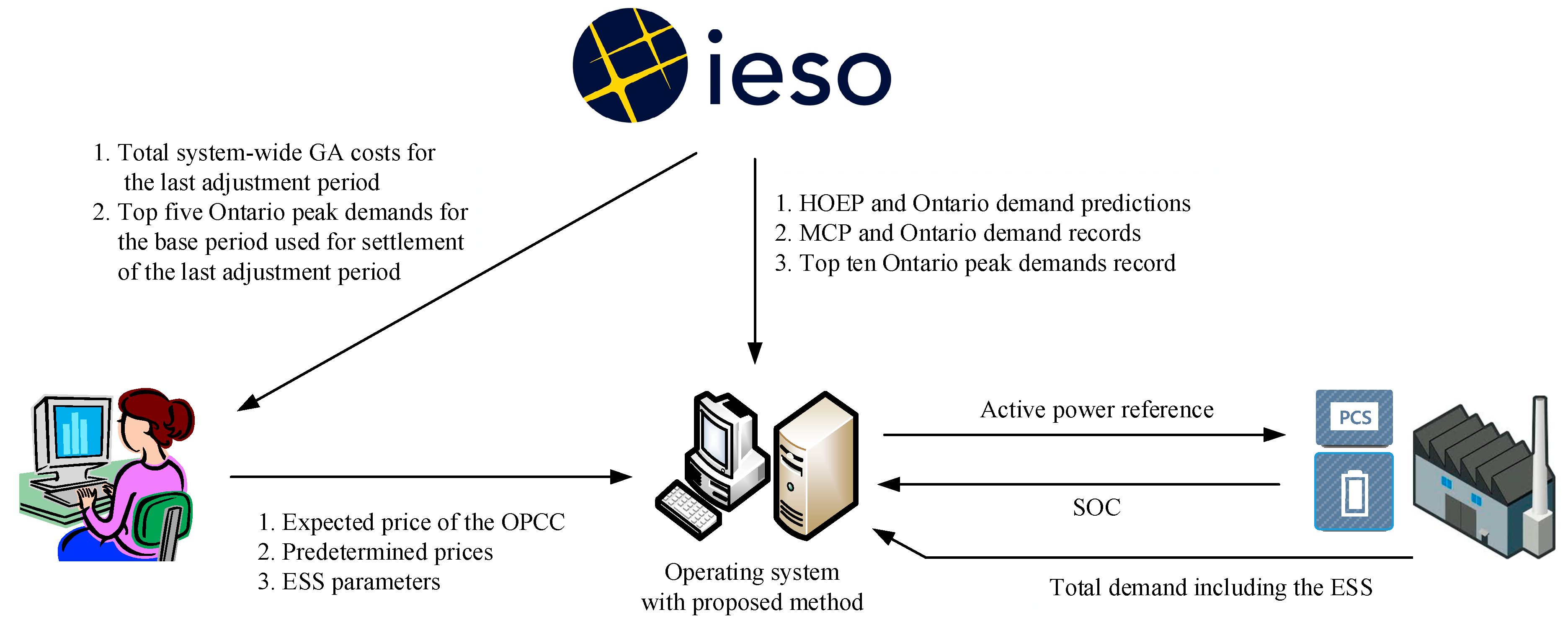
Various data are provided as files with specific types (e.g., .xml and .csv) on the website of the IESO. Among them, the following data are used for the proposed method:
- HOEP and Ontario demand predictions
- MCP and Ontario demand records
- Top ten Ontario peak demands recordThe top ten Ontario peak demands for the current base period are reported. The top ten Ontario peak demands record can be obtained from reference [29].
3. ESS Output Control Method
3.1. ESS Operation Strategy
The objective of the proposed ESS operation method is to minimize the sum of electricity charges and ESS operation costs. Like the conventional methods described in Section 1, the schedule-based operation method can be adopted because the energy capacity of the ESS is limited. In other words, the output of the ESS is scheduled iteratively based on the forecasted data with consideration of the operational bounds for the state-of-charge (SOC). The active power reference for the ESS is then determined from the scheduled value for the current time interval. As the data from the IESO website are used for scheduling, the scheduling cycle should be less than the minimum updating period of the data to reflect the most recent data as soon as possible. Therefore, the scheduling cycle for the proposed method is less than five minutes, which is the updating cycle of the MCP and five-minute average Ontario demand records.
The MEUC, HEUC, PDC, and OPCC should be considered when scheduling the ESS output as these costs can be affected by the output control of the ESS. As mentioned in the previous section, the output control does not affect the OPCC of the current month. However, the OPCC can, in the worst case, be affected after 25 months, e.g., the controls on May 2018 can be reflected in the OPCC for June 2020. To represent the overall effects of the ESS control in detail, the electricity charges for the next 25 months should be considered and the operation schedule for the next 18,000 h should be determined. As a result, this approach increases the computational burden, thus the schedule may not be determined within the time limit to reflect the most recent market data given by the IESO. Moreover, the IESO does not predict the prices and demands for such a long period and for the customer, it is almost impossible to forecast the data by itself.
Meanwhile, the IESO provides a least one-day prediction for prices and demands, e.g., at 14:00, the HOEP and Ontario demand predictions for only current day can be obtained. Therefore, the expected increase in the electricity costs caused by the ESS operation in the current day, rather than the costs for the next 25 months, are considered in the proposed scheduling problem. The expected increase in the costs, instead of the expected costs, is used to simplify the formulation of the problem as the schedule to minimize the expected costs is identical to minimizing the expected increase in the costs. In other words, in the proposed method, the expected increase in the costs caused by the ESS control is estimated. An operation schedule of the ESS for a day is then determined to minimize the sum of the expected increases and operating cost.
3.2. Expected Increases in the Costs
In this subsection, the expected increases in the costs due to the ESS control for a day are formulated. By subtracting the MEUC without the ESS from the MEUC with the ESS, the increase in the MEUC for the remaining time intervals in the day can be obtained as
Similarly, the increment in the HEUC is calculated as
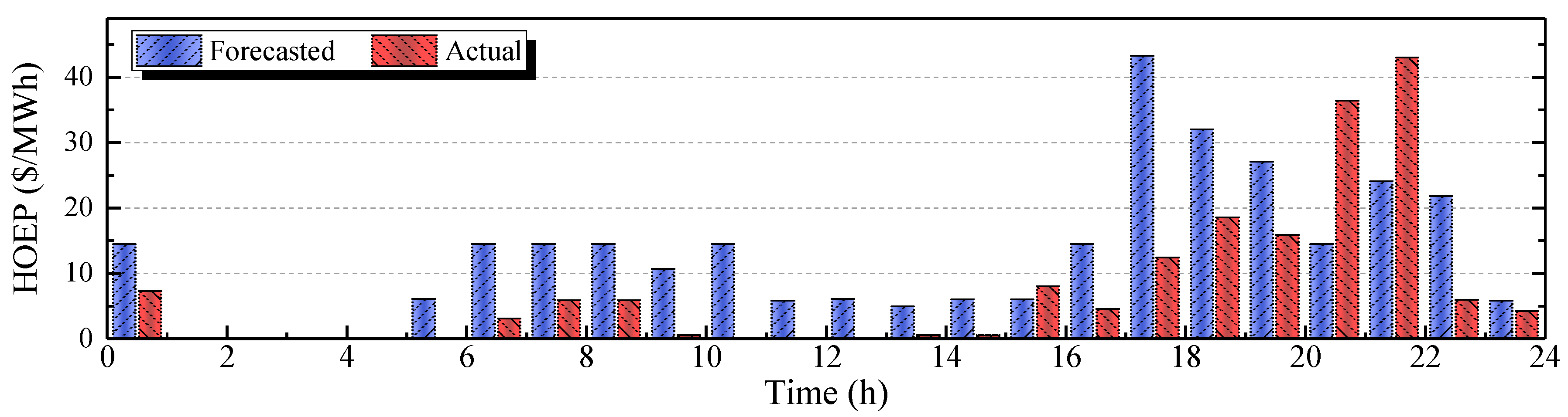
As λHEU is identical to the HOEP for the target customer, the HOEP forecasted by the IESO can be directly used as the forecasted price of HEUC, . However, as shown in Figure 1, large forecasting errors can exist in the data. The forecasted HOEP between 17 h and 18 h is about 43 $/MWh. However, the actual value is only 12 $/MWh. The forecasted HOEP between 21 h and 22 h is about 24 $/MWh, while the actual value is 43 $/MWh. This is because the forecasted HOEP is updated only until an hour before the actual operation.
It is clear that the prediction accuracy should be improved to maximize the benefits of the ESS operation. Unfortunately for the customer, it is hard to enhance the accuracy for all time intervals due to lack of information. However, it is possible to correct the forecasted HOEP for the current time interval because the actual HOEP is calculated as the average of 12 MCPs for the interval and the MCP record is provided by the IESO every five minutes. Therefore, in the proposed method, the forecasted price of HEUC for the current time interval, h, is determined as the weighted average of the HOEP forecasted by the IESO and announced MCPs for the current time interval as follows (the forecasted HOEP is directly used as the price for other intervals):
For the time intervals, except the current interval, is set as identical to the forecasted HOEP, , as the MCPs for those intervals are unknown. Similarly, for the current time interval is also set as if the number of announced MCPs, NM, for the current interval is zero. For the case when NM is positive, is determined as the weighted average of the MCPs and . As NM increases, the weight factor for decreases, thus calculated by Equation (7) is close to the actual HOEP as shown in Figure 2. In the figure, it is assumed that all MCPs are 120 $/MWh, thus the actual HOEP is also 120 $/MWh. Initially, is identical to , 50 $/MWh, because there is no MCP announced. However, increases as NM increases and is close to the actual HOEP of 120 $/MWh. Note that the actual HOEP is unknown in the current time interval as it is determined after the actual operation. In summary, the prices of the HEUC for the current time interval are corrected by using the HOEP predicted by the IESO and the MCP records to improve the forecasting accuracy. Based on this method, the ESS could be discharged in the time interval whose forecasted HOEP is low, but the actual HOEP is high, as described in Section 4.2.
The PDC is increased only if a new monthly peak demand has occurred, i.e., if the peak demand of the day is higher than the previous monthly peak demand recorded. Therefore, the expected increment of the PDC can be formulated as below:
The expected increase in the OPCC can be represented as
As the expected price of the OPCC, , is not supplied by the IESO, it can be estimated as follows. The first step is to calculate the price of the OPCC corresponding to 1 kW of demand during the top five peak hours, . Since the system-wide GA costs are distributed in proportion to the contribution to the top five peaks, can be approximated from historical data as
For example, if the operation day is 4 July 2018, CGA,LAP is the total system-wide GA cost between July 2017 and June 2018 whereas ETFOP,total is the sum of the top five Ontario demands between 1 May 2016 and 30 April 2017. These data can be obtained from the IESO webpage [30,31]. The next step is to generate the Ontario hourly demand profile forecast for the day as follows:
Note that the forecasted demand for the current interval is also corrected by using historic data given by the IESO, similar to the approach used to estimate in Equation (7). The final step is to determine for each time interval. For a day, the IESO forecasts only a single time interval that can be included in the top five peak hours as only one time interval (for which the Ontario demand is the maximum for the day) can be used for the top five peak hours. The simplest way to determine is to allocate to the peak time interval forecasted by the IESO while it is zero for other intervals. However, the prediction can be incorrect as it is not updated in real time. In addition, customers might reduce their consumption around the forecasted interval. In order to overcome this problem, is assigned to several intervals that can be one of the top five peak hours in this paper:
In Equation (12), Eth is a threshold demand and is given by the following:
where ETFOP,min is the minimum value of the current top five peak demands obtained from the top ten peak demand records given by the IESO. The concept for determining is illustrated in Figure 3. Only for the intervals between ‘a’ and ‘b’ is , while that for the other intervals is zero. If a large εth is used, Eth is decreased, thus the number of the intervals with a nonzero price, during which the ESS may be discharged to reduce the OPCC, increases. Therefore, the possibility of discharging during the top five peak hours is enhanced. However, the discharged energy during the top five peak hours is reduced due to the capacity limit of the ESS. Thus, the reduction of the OPCC is degraded. Meanwhile, in the initial part of a base period (e.g., from May to June), the recorded ETFOP,min is lower than the actual ETFOP,min for the base period. In this case, even though the predicted demand is higher than the current value of ETFOP,min, there is no need to control the ESS as the peak hour for the day will not be included in the final top five peak hours. In order to take this situation into account, EUD,min is introduced in Equation (13).
The last cost corresponds to the operating cost of the ESS. Among the various cost models, the model presented in reference [12] was utilized for the proposed method as the optimization problem can be formulated as an LP problem with a small modification. The expected increase in the operating cost is given by
where λOP is the price given by the operating cost caused by discharging/charging 1 kWh of electricity energy.
3.3. Formulation of the Scheduling Problem
The objective of the proposed method is to minimize the sum of the expected increases in electricity charges and operating cost. The problem is formulated as an optimization problem whose decision variables are energy outputs of the ESS for each time interval. From Equations (5)–(9) and (14), the objective function of the problem is expressed as
The first constraints for the problem correspond to the output limits of the ESS:
Note that the values of EESS,min and EESS,max are identical to the minimum and maximum active power limits of the ESS, respectively. As the output of the ESS should be scheduled iteratively with a cycle of less than five minutes to reflect the real-time data from the IESO, the output energy constraint for the current interval is introduced in Equation (17). For example, if the current time is 30 minutes and the already-discharged energy in the current interval is 100 kWh, the ESS with a maximum active power output of 500 kW can discharge at most 250 kWh during the remaining time of the current interval. Therefore, EESS for the current interval is limited to 350 kWh by Equation (17).
Other constraints are the SOC limits for the ESS and given by
To secure energy reserves to meet forecasting errors, Equation (19) is introduced. For example, if TSOC,max is set as 8:00, the ESS is fully charged until 8:00. Therefore, the ESS can be discharged even if unpredicted events occur in the afternoon. An actual example is addressed in the next section. Meanwhile, the SOC is calculated as
The formulated optimization problem is a nonlinear problem as it involves absolute and maximum functions in Equation (15). However, the problem can be relaxed to an LP problem with the methods presented in reference [32]. The absolute function is linearized by dividing the decision values into positive and negative terms as
Meanwhile, the maximum function in the objective function can be linearized by introducing an arbitrary value, α, as follows:
By applying these methods, the optimal scheduling problem can be formulated as a general form of an LP problem as
subject to
where x is a decision variable given by
Other variables in Equations (23) and (24) are given by
In Equation (31), A(h–TSOC,max,:) denotes the (h–TSOC,max)-th row of the matrix A.
In order to conserve the characteristic of the original problem in the LP problem, one of and should be zero. If the prices satisfy the following condition, either or is automatically set to zero.
where is given by
The detailed proof is presented in Appendix A. Otherwise, both and can be nonzero. Note that can be negative as negative HOEPs can occur in the Ontario electricity market [12]. In order to solve this problem, additional binary variables representing the charging and discharging statuses of the ESS can be used for the optimization problem [10,11,12]. However, the introduction of binary variables increases computational burden as the scheduling problem becomes a mixed integer LP problem. In the worst case, the scheduling problem cannot be solved within the five minutes that is the minimum scheduling cycle of the proposed method. Therefore, in the proposed method, the problem is solved by limiting the maximum output energy rather than by using binary variables. If the discharging increases the total costs, there is no need to discharge the ESS. In order to prevent the ESS from discharging in such cases, the modified maximum output of the ESS, EESS,max,modi in Equation (34), is determined as
The detailed procedure to derive Equation (37) is presented in Appendix B. In addition, in Appendix C, it is proven that one of and is zero by limiting the maximum output energy with Equation (37).
3.4. Determination Method for the Active Power Reference
By solving the LP problem, the optimal operation schedule can be obtained. However, an infinite number of other optimal solutions may exist if some coefficients for the objective function are identical. For example, if the ESS should discharge 100 kWh during two time intervals where the prices corresponding to the coefficient of the objective function are identical, discharging 50 kWh for each time interval can be the optimal solution. However, discharging 20 kWh in the first time interval and 80 kWh in the other time interval can also be the optimal solution as the optimal value of the objective function is the same. In this case, the solution with the flattest profile of is selected as the final schedule in the proposed method to prevent frequent changes of the schedule. In other words, the total energy output of the intervals with the same coefficient is calculated first and is then distributed equally to the intervals. With this approach, the actual losses in the ESS can be reduced as the losses are almost proportional to the square of active power.
Finally, the active power reference for the ESS is calculated from the final schedule. The scheduled output energy for the current interval, , corresponds to the total energy that should be discharged in the interval. Therefore, the active power reference, , is calculated from the scheduled energy output and the already-discharged energy, EESS,his, in the interval as shown below:
3.5. Overall Process of the Proposed Method
The overall process of the proposed method for calculating the active power reference for the ESS is illustrated in Figure 4. The process should be executed every five minutes or less to reflect the most recent data from the IESO. If the reference is determined using Equation (38), it is sent to the ESS, which controls its active power output according to the reference.
The flow of major data for the proposed method is illustrated in Figure 5. In order to reflect the most recent market data on the operation, the data with the exception of the data for the user and the user inputs are updated every five minutes at the longest.
4. Results from Case Study and Field Tests
The proposed method was verified by various case studies and actual field tests in Ontario. In this section, the major results showing the effectiveness of the proposed method are presented. For both case studies and field tests, the same 500 kWh ESS, which consisted of lithium-ion batteries, was used. The active power output of the ESS was limited to be between −500 kW and 500 kW. Based on the results of the actual field test, η+ and η– were set at 93.9% and 94.4%, respectively. The prices shown in Table 1 were calculated based on data from the websites of the IESO [30,31] and an LDC [24] were used for both the case studies and field tests. According to these prices and the fact that the HOEP is generally less than 1 $/kWh, the best scheme for discharging the ESS should first reduce the OPCC, followed by a reduction in the PDC.
4.1. Results from Case Study
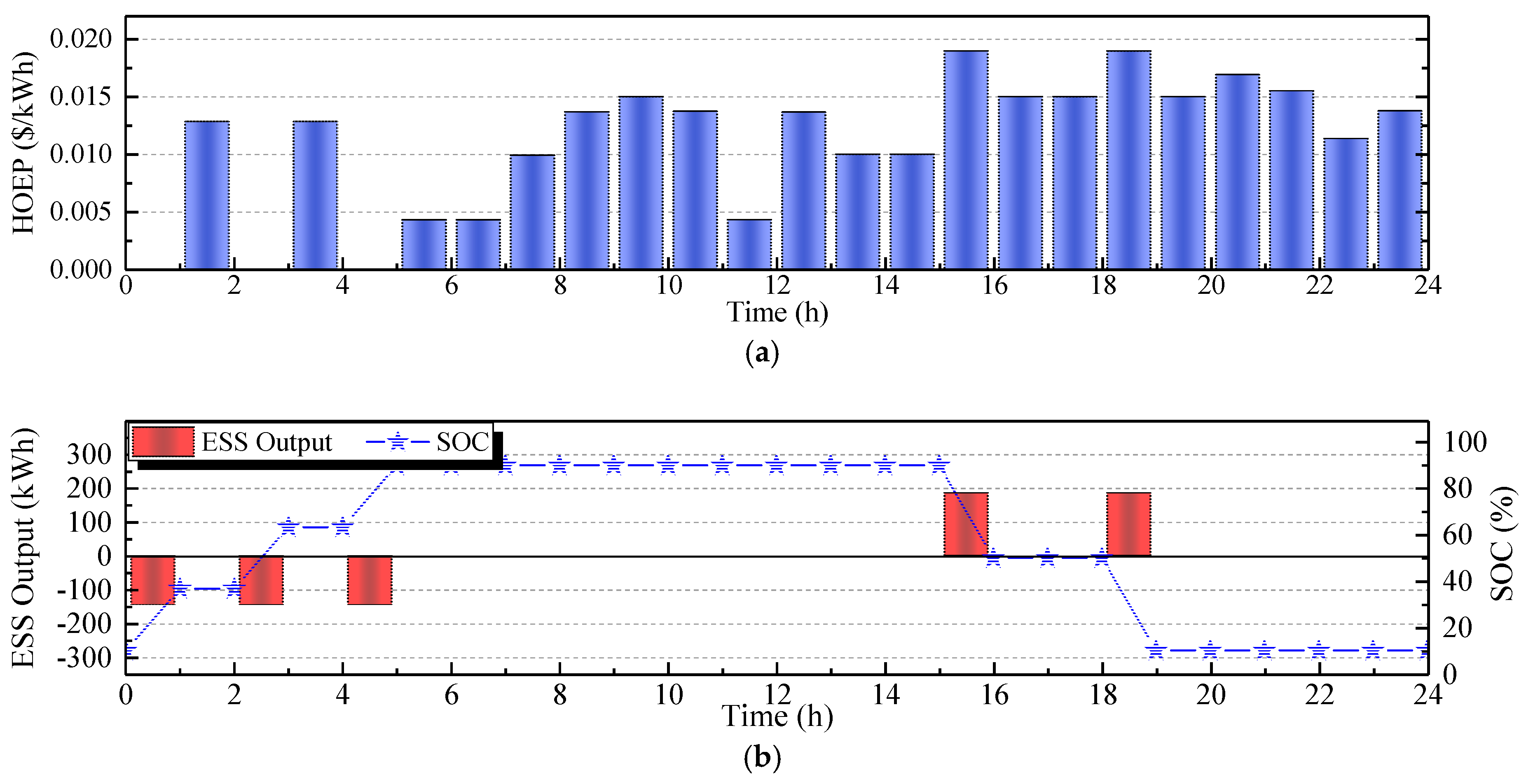
The results for the basic functions are presented in Appendix D. In this section, the results address one of the most complex cases. In the case study, it was assumed that the minimum value of the top five Ontario peak demands, ETFOP,min, and the previous peak demand of the customer, EPD,his, were 14.6 GW and 1400 kW, respectively. As shown in Figure 6a, one of the top five Ontario peak demands was predicted to occur between 19 h and 20 h, i.e., the forecasted Ontario demand was higher than the minimum value of the top five Ontario peak demands at 14.6 GW. Meanwhile, the predicted customer demand between 10 h and 14 h was larger than the previous peak demand of the customer at 1400 kW, as shown in Figure 6b. Moreover, the predicted HOEP between 16 h and 17 h was very high when compared to that of other intervals, as shown in Figure 6c. Therefore, the ESS should be discharged in the above-mentioned intervals to reduce electricity charges.
The scheduled output and SOC of the ESS with the proposed method are shown in Figure 6d and the results behaved as expected. As TSOC,max was set to 8 h, the ESS was fully charged during the time intervals when the forecasted HOEPs were minimized before 8 h and the SOC at 8 h was equal to its maximum bound of 90%. In order to reduce the peak demand, the ESS was fully discharged between 10 h and 14 h, as shown in Figure 6d. As a result, the expected peak demand could be reduced to 1457 kW from 1600 kW, as shown in Figure 6b. Between 14 h and 16 h, the ESS was charged to be subsequently discharged between 16 h and 17 h when the HOEP was high. The ESS was not, however, fully charged, i.e., the SOC at 16 h was less than 90% because more charging increases the peak demand of the customer. Note that λPD was 7.3 $/kW whereas the HOEP for the interval between 16 h and 17 h was only 0.13 $/kWh. In other words, the ESS was charged as much as possible to maximize the reduction of the HEUC while preventing an increase in the peak demand.
As the ESS should be discharged as much as possible between 19 h and 20 h, during which the Ontario peak demand was predicted, the ESS should be fully charged before 19 h to reduce the OPCC. Therefore, the ESS was partially discharged between 16 h and 17 h when the HOEP was highest, and was fully charged between 18 h and 19 h while preventing increases in the peak demand. Finally, the ESS was fully discharged between 19 h and 20 h to reduce the OPCC. With the operating schedule, it can be expected that the total cost of $42,773 could be reduced for the next 25 months as the output control of the ESS can affect the OPCC of after 25 months in the worst case scenario. The results demonstrate that the electricity charges of the customer can be reduced by using the proposed method even if the case is quite complex.
If the OPCC was not considered, the optimal schedule was as shown in Figure 7. The results before 16 h did not change, thus the peak demand of the customer was limited at 1457 kW, as shown in Figure 7a. However, the ESS was fully discharged between 16 h and 17 h, as shown in Figure 7b, where the forecasted HOEP was the highest. This is because the OPCC was not considered in this case, thus there was no need to discharge the ESS between 19 h and 20 h where the predicted Ontario demand was larger than the minimum value of the top five Ontario peak demands. With the operating schedule that did not consider the OPCC, only $1032 of the total could be reduced for the next 25 months, while $42,773 could be reduced by considering the OPCC. In other words, the proposed method could reduce the total cost more by considering the OPCC in the ESS operation.
4.2. Major Results of the Field Test
The proposed method was tested in a microgrid test bed in Penetanguishene, Ontario, Canada. The test bed was constructed in 2016 by the Korea Electric Power Cooperation and PowerStream, an LDC in Ontario. In the test bed, the proposed ESS control method was tested. The ESS was connected to the secondary side of the main circuit breaker (CB) for a distribution feeder. To test the proposed method, it was assumed that the CB was the point of common connection for a virtual customer participating in the ICI and adopting the SM rates. The active power reference for the ESS was determined every two minutes by using the proposed method.
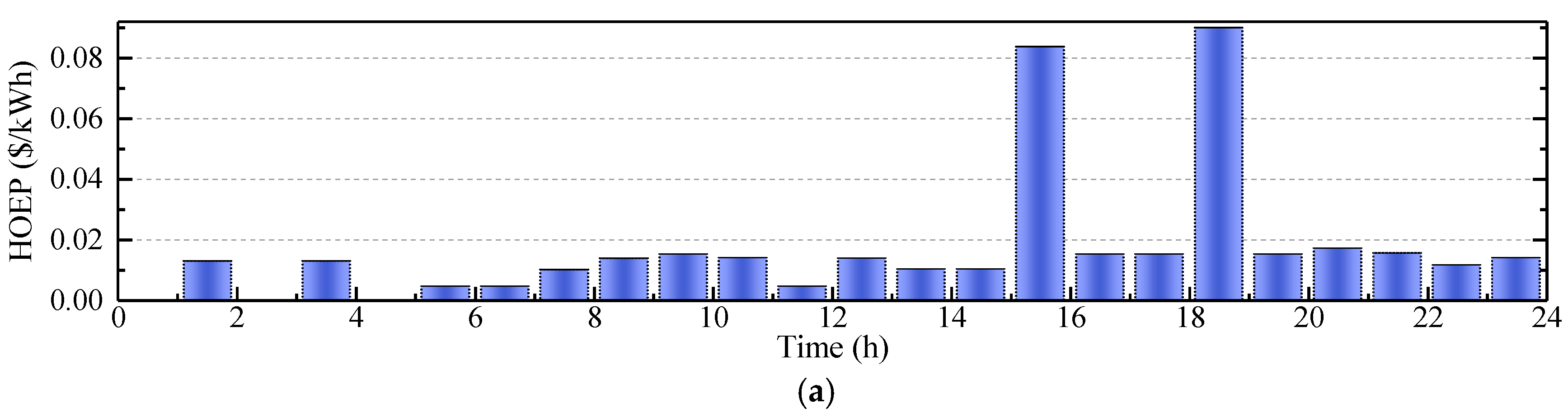
Figure 8 shows the operation results for 10 August 2016, when the largest Ontario peak demand for the base period from 1 May 2016 to 30 April 2017 occurred. As shown in Figure 8a, the IESO predicted that the Ontario peak demand would occur between 16 h and 17 h. However, the actual peak occurred between 17 h and 18 h, i.e., the predicted peak time was incorrect. Although there was an error in the predicted data, the OPCC could be reduced with the proposed method, i.e., the ESS was discharged between 17 h and 18 h when the actual peak demand occurred. The proposed method predicted a peak demand between 15 h and 18 h because the threshold reduction factor, εth, of 1% was used. Consequently, the ESS was discharged during this time interval, as shown in Figure 8b. As only 50% of the capacity, 250 kWh, was utilized by the ESS control program, about 91 kWh was discharged during the peak demand interval. Due to this operation, the OPCC for the next adjustment period could be approximately reduced by $10,220.
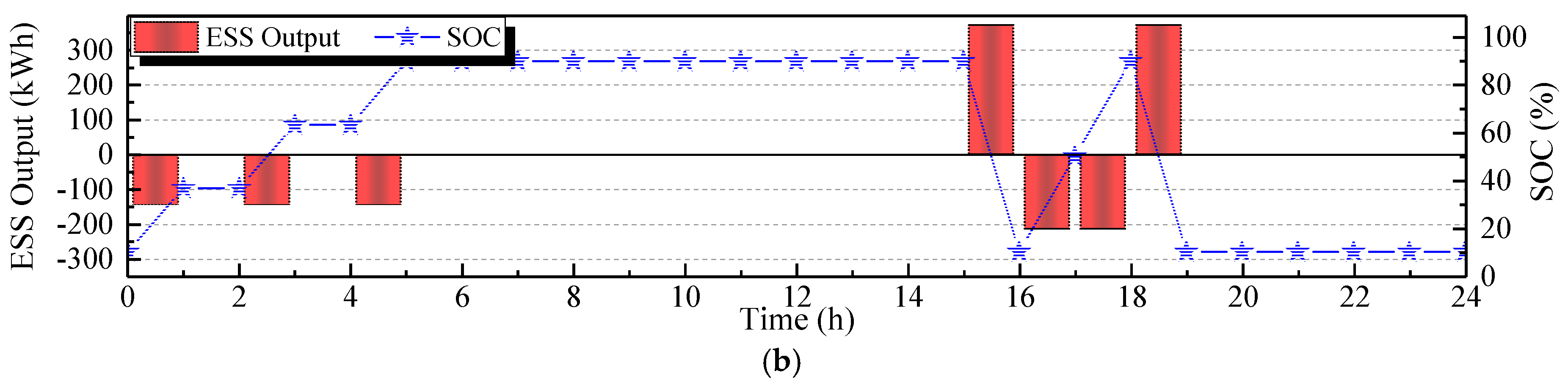
The effects of utilizing real-time data to reduce the HEUC are shown in Figure 9, which displays the operation results for 24 February 2017. With the proposed method, the ESS was charged when the HOEP was low, between 2 h and 6 h, and was subsequently discharged when the HOEP was high, between 14 h and 16 h. It is note-worthy that the ESS was almost fully discharged between 14 h and 15 h, when the actual HOEP was 279 $/MWh, which was about 14 times the average HOEP for the month, although the predicted HOEP was just 17 $/MWh. This was due to the effect of the proposed correction method using the history of MCPs. In the time interval between 14 h and 15 h, the corrected (calculated using Equation (7)) increased as the number of the announced MPCs increased, as shown in Figure 9c. Consequently, the ESS started discharging at 14 h 16 min even though the predicted HOEP was low. Due to this discharging, about $91 of the HEUC for the month could be reduced.
In addition, the ESS would not have been charged at dawn without the proposed constraint to secure energy reserves, i.e., Equation (19), as the maximum difference among the predicted HOEPs was less than twice the operating cost of the ESS, i.e., 0.06 $/kWh (=60 $/MWh), as shown in Figure 9a. However, the ESS was charged at dawn as a direct result of the proposed constraint and the ESS could be discharged when the actual HOEP was high.
5. Conclusions
A new operation method for the ESS of a customer adopting the SM rates and participating in the ICI in the Ontario electricity market was proposed to minimize the electricity charges and operation costs of the ESS. Based on the overview of the electricity charges for the target customer, it was identified that the electricity charges could be classified into five types: FC, MEUC, HEUC, PDC, and OPCC. Among them, the OPCC was the largest portion of the electricity charges, however, this has not been well reflected in previous studies. Additionally, we found that some data provided by the IESO via websites could be utilized for the ESS operation. However, there were sometimes large forecasting errors as the IESO predicts the data only until an hour before the actual operation.
Therefore, the OPCC was considered in the proposed method, i.e., the OPCC was modeled in the proposed scheduling problem and the method to determine the price of the OPCC for each time interval was presented. In order to improve the forecasting accuracy of the data for the current time interval, correction methods using the real-time records given by the IESO were proposed. In addition, the maximum SOC constraint for the scheduling problem was introduced to secure the energy reserve to react to an unpredicted event. With the proposed method, the operation schedule and the active power reference for the ESS were iteratively determined at time intervals of less than five minutes to reflect the most recent market data. From the results obtained from the case study and the actual field tests, the following conclusions could be drawn.
- The OPCC can be reduced by using the proposed method. It should be noted that it is hard to reduce the OPCC with conventional methods as the OPCC has not been previously considered in them.
- The proposed method can enable the ESS cope with unpredicted events, e.g., the ESS can be discharged in the time intervals where the actual price is high even though the price forecasted by the IESO is low.
In order to improve the performance of the proposed method, the prediction accuracy of the occurrence time of the top five Ontario peak demands, which were used to determine the price of the OPCC, should be improved. Therefore, this has been scheduled for future work.
Author Contributions
P.-I.H. proposed the main idea and wrote the paper. S.-C.K. organized and performed the field test. S.-Y.Y. supervised this work and revised the paper.
Funding
This study was supported by a research fund from Chosun University, Republic of Korea, 2017.
Conflicts of Interest
The authors declare no conflict of interest.
Nomenclature
| Acronyms | |
| ESS | Energy storage system |
| EUC | Electricity usage cost |
| FC | Fixed cost |
| GA | Global adjustment |
| HEUC | Hourly electricity usage cost |
| HOEP | Hourly Ontario energy price |
| ICI | Industrial conservation initiative |
| IESO | Independent electricity system operator |
| LDC | Local distribution company |
| LP | Linear programing |
| MCP | Market clearing price |
| MEUC | Monthly electricity usage cost |
| OPCC | Ontario peak contribution cost |
| PDC | Peak demand cost |
| SM | Spot market |
| SOC | State-of-charge |
| Variables | |
| Total system-wide GA costs for the billing month, $ | |
| Total system-wide GA costs for the last adjustment period, $ | |
| Hourly electricity usage cost, $ | |
| Monthly electricity usage cost, $ | |
| Ontario peak contribution cost, $ | |
| Energy output of an ESS, kWh | |
| Already-discharged energy for the current time interval, kWh | |
| Maximum energy output of an ESS in an hour, kWh | |
| Modified maximum output of an ESS in an hour, kWh | |
| Minimum energy output of an ESS in an hour, kWh | |
| Energy consumption of a load, kWh | |
| Ontario demand, kW | |
| Recorded Ontario demand given by the IESO, kW | |
| Previous peak demand of a customer in the current month, kW | |
| Five-minute average Ontario demand record given by the IESO, kW | |
| Rated capacity of an ESS, kWh | |
| Minimum value of the current top five peak demands, kW | |
| User-defined minimum threshold demand for the OPCC, kW | |
| Sum of the top five Ontario peak demands for the last adjustment period, kW | |
| Scheduled output energy of an ESS, kWh | |
| Discharging energy of an ESS, kWh | |
| Charging energy of an ESS, kWh | |
| n × 1 vector whose elements are equal to one | |
| Optimal energy discharged from the energy stored in the ESS, kWh | |
| Forecasted consumption of a load, kWh | |
| Ontario demand forecasted by the IESO, kW | |
| Current time interval | |
| Index of an hour-long time interval | |
| n × n identity matrix | |
| Current minute | |
| Number of time intervals remaining for the day | |
| Number of announced MCPs for the current time interval | |
| Number of five-minute average Ontario demand records announced for the current time interval | |
| n × 1 zero vector | |
| Set of time intervals included in a billing month | |
| SOC at the end of a time interval | |
| Maximum operational limit of the SOC | |
| Minimum operational limit of the SOC | |
| Set of the top five Ontario peak hours for the last base period | |
| n × n upper triangular matrix whose nonzero values are equal to one | |
| Target time interval whose final SOC should be identical to the maximum SOC | |
| Increase in the hourly electricity usage cost, $ | |
| Increase in the monthly electricity usage cost, $ | |
| Increase in the Ontario peak contribution cost, $ | |
| Increase in the operating cost, $ | |
| Threshold reduction factor | |
| Charging efficiency | |
| Discharging efficiency | |
| Hourly electricity usage price, $/kWh | |
| Market clearing price, $/kWh | |
| Monthly electricity usage price, $/kWh | |
| Operating cost of an ESS, $/kWh | |
| Peak demand price, $/kW | |
| Price of the electricity costs excepting the PDC, $/kWh | |
| Expected hourly electricity usage price, $/kWh | |
| HOEP forecasted by the IESO, $/kWh | |
| Expected price of the OPCC, $/kW | |
| Price of the OPCC, $/kW |
Appendix A. Sufficient Condition Guaranteeing That Either and Is Zero
Even though the exact value of the optimal energy discharged from the energy stored in the ESS is unknown, there will be the optimal energy for each time interval to minimize the objective function. For time interval i, the optimal energy, , can be expressed with and as
As the optimal energy is discharged from the stored energy, η+ and η– are used to represent the effects of charging and discharging losses. Meanwhile, the expected cost increase in the time interval i, f(i), can be written as follows by neglecting the PDC
where is given by
As the original problem is to minimize the costs, the problem to determine and can be expressed as the following optimization problem to minimize the costs for the current time interval.
subject to
By using Equation (A5), the objective function can be written with respect to as
As is a constant, the second term can be eliminated in the minimization problem
where is given by
Similarly, the objective function can be also written with respect to as
As is positive, the optimal solution does not change even though the objective function is divided by . As a result, Equation (A11) can be modified as
From Equations (A5)–(A7), (A9), and (A12), the optimal solution can be determined as shown in Table A1. The optimal solution for each case can be determined as follows. In Case 1, it can be identified from Equations (A9) and (A12) that both and should be minimized as is positive. Therefore, the optimal solutions correspond to the minimum values of and , which satisfy the constraints given by Equations (A5)–(A7). As is positive, the optimal and are and zero, respectively. In contrast, and should be maximized in Case 5 because is negative. As is negative in this case, is maximized first and is determined from Equation (A5).

Table A1.
Optimal and .
| Case | Optimal Solution | |||
|---|---|---|---|---|
| # | ||||
| 1 | > 0 | > 0 | 0 | |
| 2 | = 0 | 0 | 0 | |
| 3 | < 0 | 0 | ||
| 4 | = 0 | all | Infinite number of solutions | |
| 5 | < 0 | > 0 | ||
| 6 | = 0 | |||
| 7 | < 0 | |||
If is greater than zero, either or is set at zero automatically as shown in Table A1. From Equation (A10), this condition can be rewritten as
As is positive and η+ and η– are positive less than 1, the following is satisfied.
From Equations (A13) and (A14), the sufficient condition that ensures that either or is zero can be obtained as
If the PDC is considered, the sufficient condition is still valid, because is positive
In summary, if the total prices, , is not negative, either or is zero.
Appendix B. Determination of Modified Maximum Output of the ESS
If the condition given by (A15) is not guaranteed, both and can be nonzero. In order to solve this problem, the maximum output energy used for the optimization problem is modified in the proposed method. If the total costs for a time interval is increased due to discharging the ESS, there is no reason to discharge the ESS in general. Only in the case where most of the prices for time intervals are negative, the ESS may be discharged. However, this case is impractical, thus this case is not considered. Therefore, the ESS can be discharged if, and only if, the cost is maintained or decreased due to discharging.
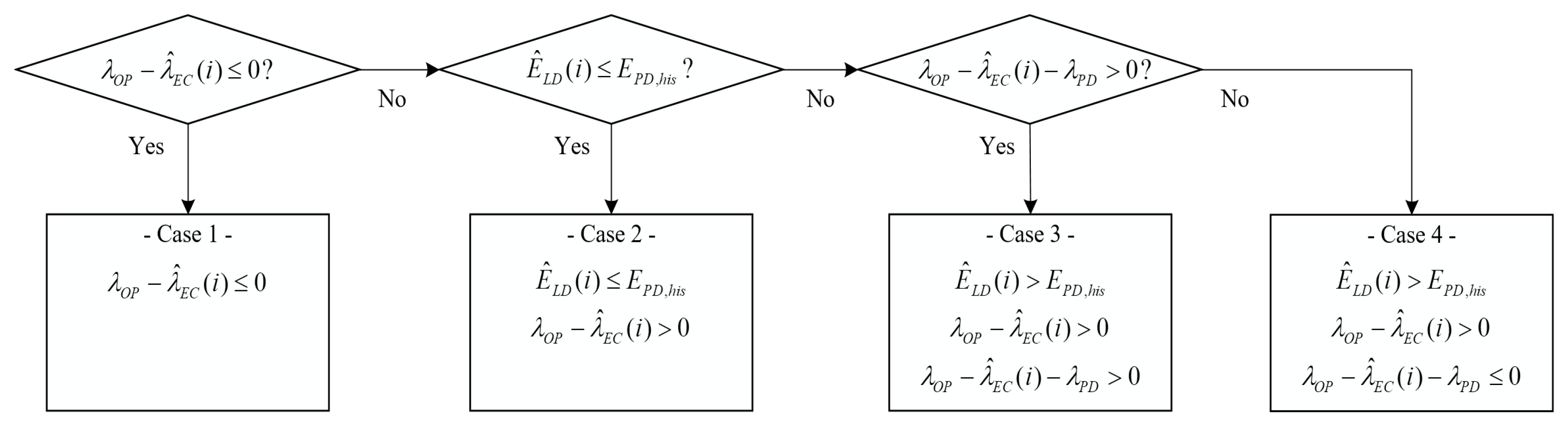
As the PDC is determined from the load of the customer, the prices and load should be considered to identify the variation of the costs. Based on the prices and load, the possible operating conditions can be classified as shown in Figure A1.
Figure A1.
Possible operating conditions.
For each case, the maximum output energy is limited as follows.
● Case 1
The variation of the costs due to charging is given by either or . As and are positive, the costs are always decreased due to the discharging of the ESS. Therefore, discharging is permitted and the maximum output energy is set at its original value, EESS,max.
● Case 2
As the load is lower than or equal to the previous peak demand, the PDC is unchanged due to discharging, thus the variation of the costs is . Meanwhile, is positive. Consequently, the costs are always increased due to discharging, thus the maximum output energy is limited to zero in this case.
● Case 3
In this case, the costs is always increased due to discharging because all possible prices are positive. Therefore, the maximum output energy is limited as zero.
● Case 4
If the total demand is smaller than the previous peak demand, i.e., , the costs are increased due to discharging because the corresponding price given by is positive. Otherwise, the costs are maintained or decreased as . Therefore, the ESS should be not discharged more than that which makes the total demand lower than the previous peak demand, i.e., . As the ESS is unable to discharge more than the original maximum output, the maximum output is limited as the smaller value of and EESS,max.
Based on these facts, the modified maximum output of the ESS, EESS,max,modi, can be determined as shown in Equation (37).
Appendix C. Proof that Equation (37) Guarantees that Either or Is Zero
In order to prove that either or is zero with the proposed method, the three cases used to determine the modified maximum output, which is shown in Equation (37), should be tested. In the first case (i.e., ), is positive as it is greater than or equal to , which is positive. Therefore, the sufficient condition given by Equation (A15), , is satisfied. If the condition for the second case is enabled, the ESS can only be discharged when the total demand, , is higher than or equal to the previous peak demand, thus is always activated. Therefore, the expected cost increase in the time interval i, f(i), can be written as
With the same process used to derive the sufficient condition in Appendix A, the following sufficient condition, which guarantees that either or is zero, when is activated can be obtained as
Meanwhile, the value of is lower than or equal to zero in the second case. This means that is positive because is positive. Therefore, the sufficient condition given by Equation (A19) is guaranteed. It is clear that is zero when the modified maximum output is zero, i.e., the third case of Equation (37). Consequently, it is guaranteed that either or is zero for all cases.
Appendix D. Simulation Results for Basic Functions
In order to verify the basic functions of the proposed method, with the exception of the response of the OPCC, the results for the following five cases are presented. Results for the first three cases represent the response to the HEUC when the predicted load demands are lower than the previous peak demand, and the others show the response to the HEUC and PDC. For all cases, the prices shown in Table 1 were used and the forecasted Ontario demands were much smaller than the minimum value of the previous top five Ontario peak demands, i.e., the expected increase in the OPCC was zero.
● Case 1
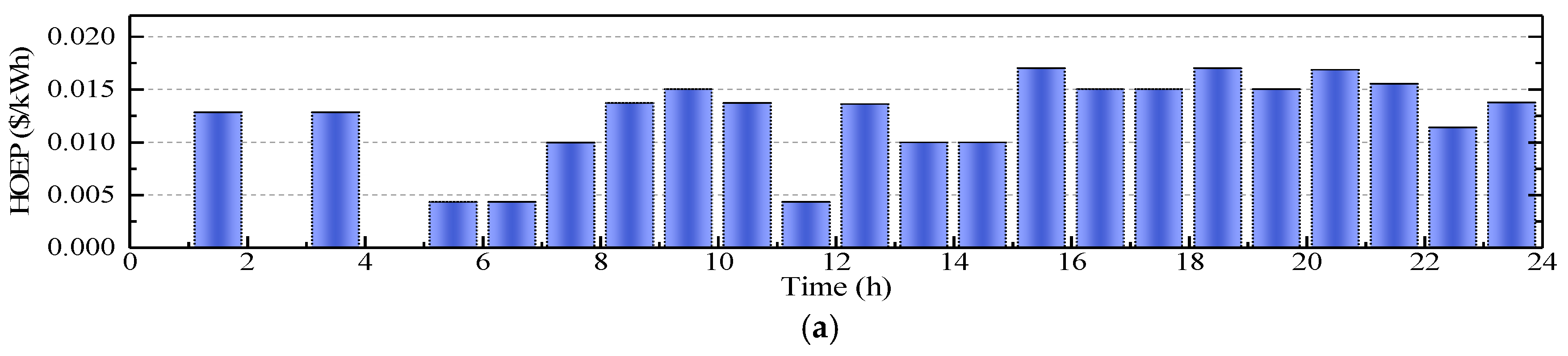
As shown in Figure A2a, the forecasted HOEPs was lower than or equal to 0.017 $/kWh, thus the maximum value of was 0.029 $/kWh (0.017 $/kWh + 0.012 $/kWh). As was 0.03 $/kWh, discharging the ESS increased the total costs. Therefore, the ESS was not scheduled for discharging as shown in Figure A2b.
Figure A2.
Results of Case 1: (a) Forecasted HOEP; (b) Scheduled output and SOC of the ESS.
● Case 2
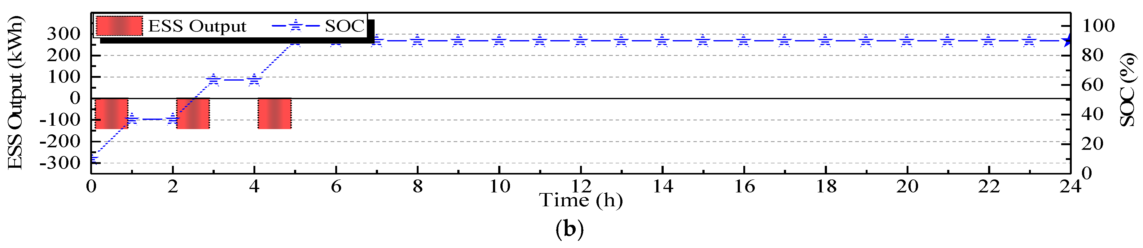
Compared with Case 1, the maximum value of the forecasted HOEP was slightly increased to 0.019 $/kWh in time intervals between 15 h and 16 h and between 18 h and 19 h, as shown in Figure A3a. As a result, for the time intervals was 0.031 $/kWh, which was larger than , 0.03 $/kWh. Therefore, the ESS was discharged in the time intervals, as shown in Figure A3b.
Figure A3.
Results of Case 2: (a) Forecasted HOEP; (b) Scheduled output and SOC of the ESS.
● Case 3
In this case, the forecasted HOEPs for time intervals between 16 h and 17 h and between 19 h and 20 h were much higher than , 0.03 $/kWh, as shown in Figure A4a. Consequently, the costs could be reduced more by (1) fully discharging between 15 h and 16 h, (2) charging between 16 h and 18 h, and (3) and fully discharging between 18 h and 19 h, as shown in Figure A4b.
Figure A4.
Results of Case 3: (a) Forecasted HOEP; (b) Scheduled output and SOC of the ESS.
● Case 4
The predicted peak demand of the customer, 1600 kW, was higher than the previous peak demand of 1550 kW, as shown in Figure A5a, and the forecasted HOEPs were lower than 0.017 $/kWh, as shown in Figure A5b. As was much higher than , the total costs could be decreased by reducing the peak demand. However, discharging that did not reduce the peak demand increased the costs, like in Case 1. Therefore, as shown in Figure A5c, the ESS was discharged in the time intervals where the predicted demand was larger than the previous peak demand, i.e., time intervals between 10 h and 11 h and between 12 h and 13 h. As discharging more in these intervals increased the costs, the ESS was only discharged when making the demands identical to the previous peak demand, i.e., the peak demand shown in Figure A5a was reduced to 1550 kW by discharging 50 kWh for each time interval.
Figure A5.
Results of Case 4: (a) Customer demand; (b) Forecasted HOEP; (c) Scheduled output and SOC of the ESS.
Figure A5.
Results of Case 4: (a) Customer demand; (b) Forecasted HOEP; (c) Scheduled output and SOC of the ESS.

● Case 5
The predicted demands were the same as those of Case 4, as shown in Figure A6a, but the forecasted HOEP for the time interval between 12 h and 13 h was much higher than , 0.03 $/kWh, as shown in Figure A6b. This implies that discharging more in this time interval could decrease the total costs more than that in Case 4. Consequently, the ESS was scheduled to be discharged more in the time interval, as shown in Figure A6c.
Figure A6.
Results of Case 5: (a) Customer demand; (b) Forecasted HOEP; (c) Scheduled output and SOC of the ESS.
Figure A6.
Results of Case 5: (a) Customer demand; (b) Forecasted HOEP; (c) Scheduled output and SOC of the ESS.

From the results, it can be concluded that the proposed method responded to the HEUC and PDC appropriately.
References
- Mercier, P.; Cherkaoui, R.; Oudalov, A. Optimizing a battery energy storage system for frequency control application in an isolated power system. IEEE Trans. Power Syst. 2009, 24, 1469–1477. [Google Scholar] [CrossRef]
- Beaudin, M.; Zareipour, H.; Schellenberglabe, A.; Rosehart, W. Energy storage for mitigating the variability of renewable electricity sources: An updated review. Energy Sustain. Dev. 2010, 14, 302–314. [Google Scholar] [CrossRef]
- Sahay, K.; Dwivedi, B. Supercapacitors energy storage system for power quality improvement: An overview. J. Energy Sources 2009, 10, 1–8. [Google Scholar]
- Lee, T.Y. Operating schedule of battery energy storage system in a time-of-use rate industrial user with wind turbine generators: A multipass iteration particle swarm optimization approach. IEEE Trans. Energy Conver. 2007, 22, 774–782. [Google Scholar] [CrossRef]
- Chacra, F.A.; Bastard, P.; Fleury, G.; Clavreul, R. Impact of energy storage costs on economical performance in a distribution substation. IEEE Trans. Power Syst. 2005, 24, 684–691. [Google Scholar] [CrossRef]
- Adamek, F.; Arnold, M.; Andersson, G. On decisive storage parameters for minimizing energy supply costs in multicarrier energy systems. IEEE Trans. Sustain. Energy 2014, 5, 102–109. [Google Scholar] [CrossRef]
- Wang, Y.; Lin, X.; Pedram, M. A near-optimal model-based control algorithm for households equipped with residential photovoltaic power generation and energy storage systems. IEEE Trans. Sustain. Energy 2016, 7, 77–86. [Google Scholar] [CrossRef]
- Chen, C.; Duan, S.; Cai, T.; Liu, B.; Hu, G. Smart energy management system for optimal microgrid economic operation. IET Renew. Power Gener. 2011, 5, 258–267. [Google Scholar] [CrossRef]
- Mahmoodi, M.; Shamsi, P.; Fahimi, B. Economic dispatch of a hybrid microgrid with distributed energy storage. IEEE Trans. Smart Grid 2015, 6, 2607–2614. [Google Scholar] [CrossRef]
- Khani, H.; Zadeh, M.R.D.; Seethapathy, R. Large-scale energy storage deployment in ontario utilizing time-of-use and wholesale electricity prices: An economic analysis. In Proceedings of the Cigre Canada Conference, Toronto, ON, Canada, 22–24 September 2014; pp. 1–8. [Google Scholar]
- Khani, H.; Zadeh, M.R.D. Online adaptive real-time optimal dispatch of privately owned energy storage systems using public-domain electricity market prices. IEEE Trans. Power Syst. 2015, 30, 930–938. [Google Scholar] [CrossRef]
- Khani, H.; Varma, R.K.; Zadeh, M.R.D.; Hajimiragha, A.H. A real-time multistep optimization-based model for scheduling of storage-based large-scale electricity consumers in a wholesale market. IEEE Trans. Sustain. Energy 2017, 8, 836–845. [Google Scholar] [CrossRef]
- Xu, Y.; Tong, L. On the operation and value of storage in consumer demand response. In Proceedings of the 53rd IEEE Conference Decision Control (CDC), Los Angeles, CA, USA, 15–17 December 2014; pp. 205–210. [Google Scholar]
- Mokrian, P.; Stephen, M. A stochastic programming framework for the valuation of electricity storage. In Proceedings of the 26th USAEE/IAEE North America Conference, Ann Arbor, MI, USA, 24–27 September 2006; pp. 24–27. [Google Scholar]
- Qin, J.; Sevlian, R.; Varodayan, D.; Rajagopal, R. Optimal electric energy storage operation. In Proceedings of the IEEE PES GM, San Diego, CA, USA, 22–26 July 2012; pp. 1–6. [Google Scholar]
- Erdinc, O.; Paterakis, N.G.; Mendes, T.D.P.; Bakirtzis, A.G.; Catalao, J.P.S. Smart household operation considering bi-directional EV and ESS utilization by real-time pricing-based DR. IEEE Trans. Smart Grid 2015, 6, 1281–1291. [Google Scholar] [CrossRef]
- Van de Ven, P.M.; Hegde, N.; Massoulie, L.; Salonidis, T. Optimal control of end-user energy storage. IEEE Trans. Smart Grid 2013, 4, 789–797. [Google Scholar] [CrossRef]
- Lujano-Rojas, J.M.; Dufo-López, R.; Bernal-Agustín, J.L.; Catalão, J.P.S. Optimizing daily operation of battery energy storage systems under real-time pricing schemes. IEEE Trans. Smart Grid 2017, 8, 316–330. [Google Scholar] [CrossRef]
- Yoon, Y.; Kim, Y.-H. Effective scheduling of residential energy storage systems under dynamic pricing. Renew. Energy 2016, 87, 936–945. [Google Scholar] [CrossRef]
- Zhang, L.; Li, Y. Optimal energy management of wind-battery hybrid power system with two-scale dynamic programming. IEEE Trans. Sustain. Energy 2013, 4, 765–773. [Google Scholar] [CrossRef]
- Nguyen, M.Y.; Nguyen, D.H.; Yoon, Y.T. A new battery energy storage charging/discharging scheme for wind power producers in realtime markets. Energies 2012, 5, 5439–5452. [Google Scholar] [CrossRef]
- Telaretti, E.; Ippolito, M.; Dusonchet, L. A simple operating strategy of small-scale battery energy storages for energy arbitrage under dynamic pricing tariffs. Energies 2016, 9, 1–20. [Google Scholar] [CrossRef]
- Ontario Energy Report. ONTARIO ENERGY REPORT Q4 2017. Available online: https://www.ontarioenergyreport.ca/pdfs/6210_IESO_2017Q4OER_Electricity_EN.pdf (accessed on 20 September 2018).
- Power Stream Website. Rates & Support Programs. Available online: https://www.powerstream.ca/customers/rates-support-programs.html (accessed on 18 January 2018).
- Independent Electricity System Operator (IESO). Understanding Global Adjustment. Available online: http://ieso.ca/-/media/files/ieso/document-library/global-adjustment/understanding-global-adjustment.pdf (accessed on 18 January 2018).
- Independent Electricity System Operator (IESO). Industrial Conservation Initiative Backgrounder September 2017. Available online: http://ieso.ca/-/media/files/ieso/document-library/global-adjustment/ici-backgrounder.pdf (accessed on 4 September 2018).
- Independent Electricity System Operator (IESO). Price. Available online: http://ieso.ca/-/media/files/ieso/uploaded/chart/price_multiday.xml (accessed on 20 July 2018).
- Independent Electricity System Operator (IESO). Demand. Available online: http://ieso.ca/-/media/files/ieso/uploaded/chart/ontario_demand_multiday.xml (accessed on 20 July 2018).
- Independent Electricity System Operator (IESO). Peak Tracker. Available online: http://ieso.ca/-/media/files/ieso/power-data/peak-tracker.xml (accessed on 20 July 2018).
- Independent Electricity System Operator (IESO). Top Ten Ontario Demand Peaks Archive. Available online: http://ieso.ca/-/media/files/ieso/settlements/top-ten-ontario-demand-peaks-archive.xlsx (accessed on 23 January 2018).
- Independent Electricity System Operator (IESO). Global Adjustment Components and Costs. Available online: http://ieso.ca/en/sector-participants/settlements/global-adjustment-components-and-costs (accessed on 23 January 2018).
- Paragon Decision Technology. AIMMS Optimization Modeling. Available online: https://download.aimms.com/aimms/download/manuals/AIMMS3_OM.pdf (accessed on 18 January 2018).
Figure 1.
Forecasted and actual hourly Ontario energy price (HOEPs) on 23 December 2016.

Figure 2.
Concept of the correction method to improve the forecasting accuracy of for the current time interval.
Figure 2.
Concept of the correction method to improve the forecasting accuracy of for the current time interval.

Figure 3.
Concept for determining .

Figure 4.
Overall process of the proposed method.

Figure 5.
Flow of the major data.

Figure 6.
Results of the case study with the proposed method: (a) Forecasted Ontario demand; (b) Customer demand; (c) Forecasted HOEP; (d) Scheduled output and state-of-charge (SOC) of the energy storage system (ESS).
Figure 6.
Results of the case study with the proposed method: (a) Forecasted Ontario demand; (b) Customer demand; (c) Forecasted HOEP; (d) Scheduled output and state-of-charge (SOC) of the energy storage system (ESS).

Figure 7.
Results of the case study without considering the Ontario peak contribution cost (OPCC): (a) Customer demand; (b) Scheduled output and SOC of the ESS.
Figure 7.
Results of the case study without considering the Ontario peak contribution cost (OPCC): (a) Customer demand; (b) Scheduled output and SOC of the ESS.

Figure 8.
Actual operation results for August 10, 2016: (a) forecasted and actual Ontario demands; (b) output and SOC of the ESS.
Figure 8.
Actual operation results for August 10, 2016: (a) forecasted and actual Ontario demands; (b) output and SOC of the ESS.

Figure 9.
Actual operation results for February 24, 2017: (a) Forecasted and actual HOEPs; (b) Active power output and SOC of the ESS; (c) MPCs between 14 h and 15 h; (d) Active power output between 14 h and 15 h.
Figure 9.
Actual operation results for February 24, 2017: (a) Forecasted and actual HOEPs; (b) Active power output and SOC of the ESS; (c) MPCs between 14 h and 15 h; (d) Active power output between 14 h and 15 h.
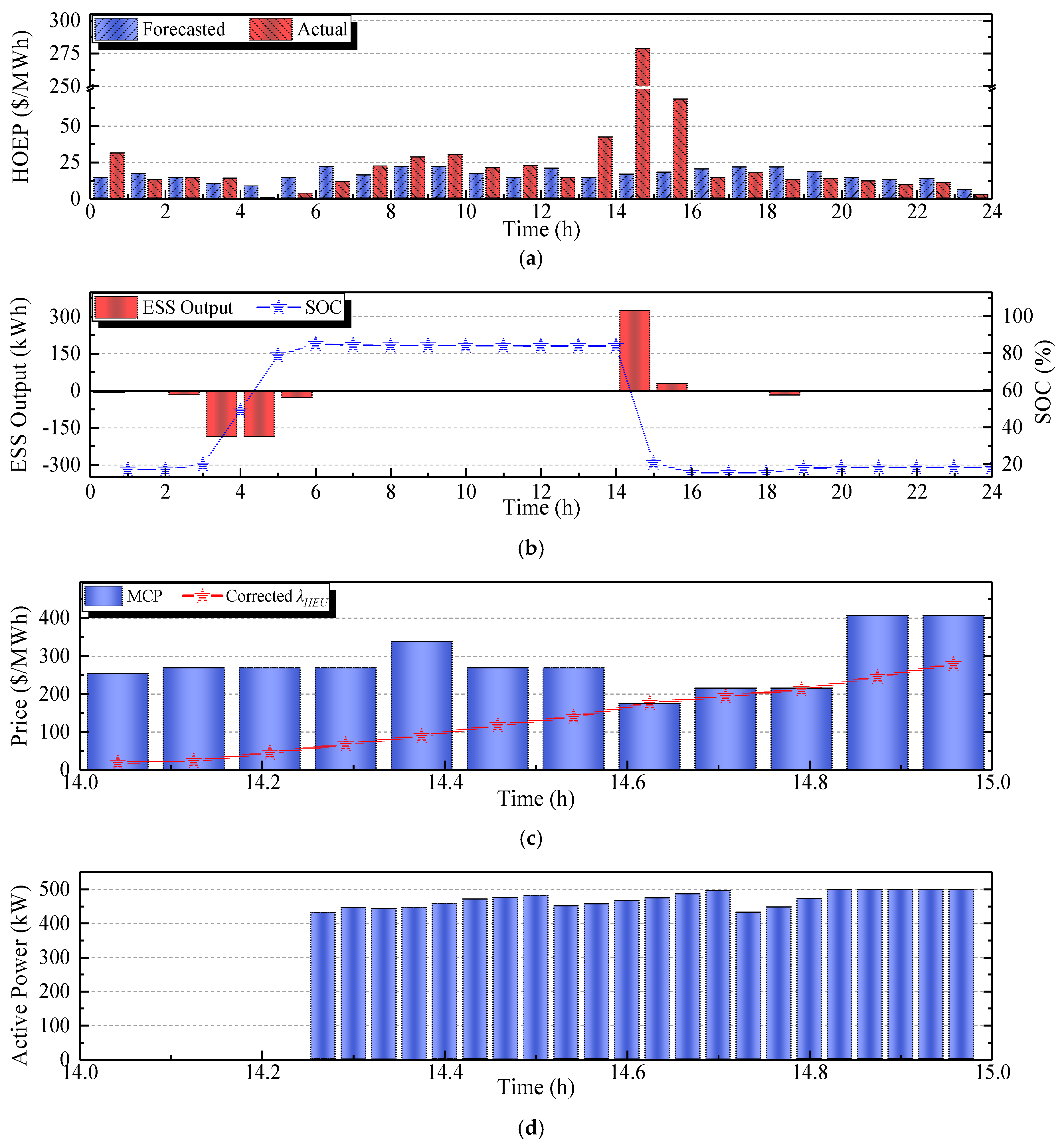
Table 1.
Prices used for the simulation and field test.
| Price | ||||
|---|---|---|---|---|
| Value | 0.012 $/kWh | 7.3 $/kW | 112.3 $/kW | 0.03 $/kWh |
© 2018 by the authors. Licensee MDPI, Basel, Switzerland. This article is an open access article distributed under the terms and conditions of the Creative Commons Attribution (CC BY) license (http://creativecommons.org/licenses/by/4.0/).
Share and Cite
MDPI and ACS Style
Hwang, P.-I.; Kwon, S.-C.; Yun, S.-Y. Schedule-Based Operation Method Using Market Data for an Energy Storage System of a Customer in the Ontario Electricity Market. Energies 2018, 11, 2683. https://doi.org/10.3390/en11102683
AMA Style
Hwang P-I, Kwon S-C, Yun S-Y. Schedule-Based Operation Method Using Market Data for an Energy Storage System of a Customer in the Ontario Electricity Market. Energies. 2018; 11(10):2683. https://doi.org/10.3390/en11102683
Chicago/Turabian StyleHwang, Pyeong-Ik, Seong-Chul Kwon, and Sang-Yun Yun. 2018. "Schedule-Based Operation Method Using Market Data for an Energy Storage System of a Customer in the Ontario Electricity Market" Energies 11, no. 10: 2683. https://doi.org/10.3390/en11102683
Note that from the first issue of 2016, this journal uses article numbers instead of page numbers. See further details here.