Extreme Learning Machines for Solar Photovoltaic Power Predictions


1
Department of Mechanical and Maintenance Engineering, School of Applied Technical Sciences, German Jordanian University, Amman 11180, Jordan
2
Department of Mechanical Engineering, School of Engineering, The University of Jordan, Amman 11942, Jordan
3
Renewable Energy Center, Applied Science Private University, Amman 11931, Jordan
*
Author to whom correspondence should be addressed.
Energies 2018, 11(10), 2725; https://doi.org/10.3390/en11102725
Submission received: 3 September 2018
/
Revised: 7 October 2018
/
Accepted: 9 October 2018
/
Published: 11 October 2018
(This article belongs to the Special Issue Solar and Wind Energy Forecasting)
Abstract
:The unpredictability of intermittent renewable energy (RE) sources (solar and wind) constitutes reliability challenges for utilities whose goal is to match electricity supply to consumer demands across centralized grid networks. Thus, balancing the variable and increasing power inputs from plants with intermittent energy sources becomes a fundamental issue for transmission system operators. As a result, forecasting techniques have obtained paramount importance. This work aims at exploiting the simplicity, fast computational and good generalization capability of Extreme Learning Machines (ELMs) in providing accurate 24 h-ahead solar photovoltaic (PV) power production predictions. The ELM architecture is firstly optimized, e.g., in terms of number of hidden neurons, and number of historical solar radiations and ambient temperatures (embedding dimension) required for training the ELM model, then it is used online to predict the solar PV power productions. The investigated ELM model is applied to a real case study of 264 kWp solar PV system installed on the roof of the Faculty of Engineering at the Applied Science Private University (ASU), Amman, Jordan. Results showed the capability of the ELM model in providing predictions that are slightly more accurate with negligible computational efforts compared to a Back Propagation Artificial Neural Network (BP-ANN) model, which is currently adopted by the PV system owners for the prediction task.
1. Introduction
Jordan is an emerging middle eastern country. Unlike other neighbouring countries, Jordan is non-oil producing with limited natural resources. The overall production of natural gas and crude oil covers less than 4% of the total national energy demand. The imported energy resources are a major burden on the country’s national economy. As a yearly average in the last four years, Jordan was spending more than 10% of its Gross Domestic Product (GDP) to cover the cost of achieving its energy demands with a large share focused on electricity generation [1,2,3,4,5].
Electricity consumption is growing due to increasing industrialization and fast-growing population; the latter is related to natural growth as well as due to refugees from Syria and Iraq. Between 2005 and 2015, the peak power demand as well as the consumption of electrical energy have increased noticeably (Figure 1). For example, the peak power increased from 1287 MW in 2005 to 3088 MW in 2015. In parallel, the overall consumed electrical energy increased from 8.8 TWh in 2005 to 15.4 TWh in 2015. Within that period, the annual average growth rate of the peak power demand and the corresponding yearly consumption of electrical energy were roughly 180 MW/a and 0.66 TWh/a, respectively. In this context, Jordan had recognized the need to invest in renewable energy (RE). Based on the 2007–2020 energy strategy, and the updated “Jordan 2025 a national vision and strategy”, it has been planned to increase the share of renewables in the energy mix to 10% in 2020 [6,7].
Solar photovoltaic (PV) systems in Jordan have evolved from being a niche market of small-scale applications used for remote power systems towards becoming a MW-scale that feed significant energy into the utility grid. Currently, the share of installed generating capacity of RE systems (solar and wind) accounts for 10% of the total installed capacity, as shown in Figure 2 [8]. However, the stochasticity (variability) of RE sources have brought technical challenges to grids, espcieally to the Transmission Network Service Provider (TNSP) [1,8,9,10].
To manage and control the country’s electricity grid, Jordan follows the single-buyer model shown in Figure 3. National Electric Power Company (NEPCO), as TNSP, is responsible of energy trading with all interconnected parties on the grid: four private entities and one governmental entity have been licensed to own and operate the conventional power plants, which generate the required electricity to cover the country’s demands. The distribution of the electricity to final consumers for the southern, northern, and central parts of the country is carried out by three entities, which are, respectively: (i) the Electricity Distribution Company (EDCO); (ii) Irbid District Electricity Company (IDECO); and (iii) Jordan Electric Power Company (JEPCO). The interconnection among these categories is illustrated in Figure 3 (simplified from [12]).
One vital activity of the TNSP is to prepare a day ahead plan for loading the running power generation units differently, to cover the needed system demand with the most economic manner according to the order of merits. Meanwhile, the TNSP is accustomed to managing the variability and uncertainty in the load with economic dispatch. The unpredictability of intermittent RE energy sources creates reliability challenges for utilities aiming at balancing power supplies and demands across centralized grid networks. Thus, balancing more of the variable input of renewables become a major challenge for TNSP, and prediction (forecasting) methods and tools are required in order to facilitate the integration of high penetration of variable RE input [13,14,15,16,17,18,19,20].
2. Literature Review
Approaches for solar photovoltaic (PV) power predictions are broadly classified into model-based and data-driven [19,21]. The former approaches employ physics-based models that use weather variables (e.g., solar radiations, temperatures, wind speed, etc.) for the solar power predictions [22]. Although these approaches lead to accurate prediction results, but uncertainty arising due to the simplifications and assumptions in the adopted models may pose constraints on their practical deployment [19,20,23].
Contrarily, data-driven approaches, such as those based on Machine Learning (ML) techniques, do not use any physics-based models, but rely solely on the availability of solar data to build black-box models for capturing the relationship of weather variables and solar PV power productions [19,24]. For example, Chow et al. [25], have employed the Artificial Neural Network (ANN) technique to capture the nonlinear relationship between the metrological variables and the energy produced by a PV system. It was found that the solar radiation, solar elevation and azimuth angles, and dry-bulb temperature are capable of effectively predicting the PV energy production; Omar et al. [26], have developed ensembles of multilayer perceptron feedforward ANNs models for 24 h-ahead power prediction of a solar facility using the forecasted weather variables of the next day; Ding et al. [27], have proposed an improved Back Propagation (BP) learning algorithm within an ANN for accurate 24 h-ahead solar PV power predictions, under different weather conditions; Mandal et al. [28], have explored the combination of Wavelet Transform (WT) and Radial Basis Function Neural Network (RBFNN) techniques for accurate 1 h-ahead PV power output forecasting: the spike changes in PV power time-series data have been filtered by resorting to WT, and the nonlinear fluctuation of PV power has been captured with RBFNN.
Bouzerdoum et al. [29], have developed a new hybrid Seasonal Auto-Regressive Integrated Moving Average (SARIMA) and Support Vector Machines (SVMs) model for short-term power forecasting of a grid-connected PV. The developed model has been shown capable of providing more robust and accurate predictions than any of the two individual models. In [30], the authors have proposed a novel statistical short-term forecasting system for hourly energy production in a real, grid-connected, PV plant. The proposed system comprises two Numerical Weather Prediction (NWP) models for forecasting the weather variables, and an Artificial Intelligence (AI)-based model (i.e., k-NN, ANN, ARIMA, and ANFIS) for 1–39 h-ahead solar power predictions, based on the forecasted weather data. Alomari et al. [31], have presented an ANN-based forecasting model that used the measured weather and PV power data for 24 h-ahead power predictions. The presented ANN model has been further enhanced by exploring two learning algorithms, namely the Levenberg-Marquardt and Bayesian Regularization, for the purpose of correlating the historical weather variables to the PV power productions [32]. Behera et al. [33] have proposed a modified Extreme Learning Machine (ELM) technique for PV power forecasting, whose weights have been tuned by resorting to different Particle Swarm Optimization (PSO) techniques. The obtained results have been compared to those obtained by the state-of-the-art BP-ANN forecasting model.
Among the existing data-driven techniques, the ELM is a new learning algorithm for single-hidden layer feedforward neural networks, originally developed by [34]. It has gained an increasing interest in different industrial applications due to its simplicity, fast computational and good generalization capability [34]. Differently from the conventional BP-ANN, the internal parameters of ELM are generated randomly (i.e., weights of the input-hidden layers) and calculated analytically (i.e., weights of the hidden-output layers), whereas the BP-ANN employs the well-known BP algorithm to iteratively set its internal parameters, leading to large computational demands.
To the best of our knowledge, few efforts have been dedicated for investigating the capability of the ELM data-driven model in predicting solar PV power production. Therefore, the objectives of the present work are two-fold:
- The development of empirical, data-driven prediction model based on the ELM, that receives in input the historical global solar radiation and ambient temperature values and provides in output the 24 h-ahead prediction of the PV system power production. The ELM model is optimized in terms of number of hidden layer neurons, hidden neuron activation function and number of historical global solar radiation values needed for accurate predictions (hereafter called embedding dimension);
ELM and BP-ANN are both applied to a real case study concerning measured real weather and production data taken from a 264 kWp solar PV system installed on the roof of the Faculty of Engineering at Applied Science Private University (ASU) in Jordan [35]. The original contribution of this work is the development and the application of optimum ELM model for the solar power production prediction task and its comparison with BP-ANN model employed by the PV system owners [31,32]. The performances of the prediction models are verified with respect to three standard metrics [20,36], namely Root Mean Square Error (RMSE), Mean Absolute Error (MAE), and Weighted Mean Absolute Error (WMAE) in addition to the time necessary for building/training the prediction models.
The remaining of this paper is structured as follows. In Section 3, the ASU solar PV system case study is illustrated. In Section 4 and Section 5, the results of the application of the ELM model to the case study are presented and compared with those obtained by the BP-ANN model of the system owners, respectively. Finally, some conclusions are drawn in Section 6.
3. Case Study: ASU Solar PV System
In this Section, a real case study of a solar PV system of a capacity of 264 kWp installed on the roof of the Faculty of Engineering at ASU, Amman, Jordan (whose coordinates location (latitude, longitude) is 32°2′24.0324″ N and 35°54′1.4328″ E) is presented [35].
3.1. Data Description
The dataset extracted from the PV system in the ASU campus comprises (i) real weather data measured by an existing weather station located around 171 m from the Faculty of Engineering, , and (ii) the corresponding power productions (in kW) measured and recorded by the inverters of the PV system, (Figure 4 [37]) [35].
The dataset used in this work has been collected in the period of three years (from 16 May 2015 to 30 September 2017) on an hourly basis, i.e., with a time step h, i.e., from 0 a.m. to 11 p.m. daily. The weather data, , include the hourly measurements of 45 weather variables, e.g., wind speeds and directions, humidity, global radiation, precipitation, and temperature at different heights in the plant, whereas the power production data include the mean power productions obtained by the PV system (in kW).
It is worth mentioning that among the 45 weather variables, few variables show constant values during the three-year period and, hence, they are excluded from the analysis. Among the remaining weather variables, engineering and expert judgment suggested to use the global solar radiation, (in W/m2), and the ambient temperature at 1 m altitude, (in °C), as the weather variables that have the largest influence on the solar PV power productions, [19,31,32]. The investigation of the influence of the remaining weather variables on the power productions predictions could be an object of future research work.
For clarification purposes, Figure 5 shows the hourly global solar radiation values (top left), the hourly ambient temperature values at 1 m altitude (top right) and the corresponding solar power productions (bottom) of the 2016-year data. For confidentiality reasons, throughout the paper, the values of the solar radiations, ambient temperatures and energy productions reported in the Figures are given on an arbitrary scale. From Figure 5, it can be easily recognized that [19]:
- The large variability in the global solar radiation and ambient temperature of the system, at the different days of the year, and the corresponding large variability of the power productions.
3.2. Data Pre-Processing
For proper use of the dataset for the prediction task, the following pre-processes have been carried out on the three-year dataset:
- Negative values and associated missing values have been recognized in the early morning (i.e., 0 a.m.–6 a.m.) and in the late evening (i.e., 6 p.m.–11 p.m.) times, due to radiation measurement devices (i.e., offset in the sensors) and inverter failures, respectively. Correspondingly, the values and the associated values are set to 0;
- A few values were not reported correctly at some time instants, due to temperature measurement devices failures (i.e., offset in the sensors). Correspondingly, they are treated as missing values and, thus, they have been excluded from the analysis with the corresponding and values;
- Missing , values and/or missing values have been recognized in some days of the dataset, due to radiation and temperature measurement devices failures and some network connection disruptions and/or inverter failures, respectively. Correspondingly, the and values and the associated values in both cases are excluded from the analysis;
For the solar PV power production prediction task, the three-year dataset is partitioned into:
- Training, , and validation, , datasets that contain the global solar radiation values, , and the corresponding power productions, , sampled randomly from the 2015–2016 years data with fractions of 60% and 40%, respectively. The training dataset is formed by patterns, which are used for building/training the ELM (Section 4) and the ANN (Section 5) prediction models, whereas the validation dataset is formed by patterns, which are used for optimizing the architectures of ELM (Section 4) and ANN (Section 5) prediction models;
- Test dataset, , that contains the 2017-year data, which have never been, used during the development of the prediction models. The test dataset is formed by patterns, which are used to evaluate the performance of the optimum ELM prediction model with respect to that of the ANN prediction model.
It is worth mentioning that each pattern of the created datasets comprises in inputs the historical real radiation and ambient temperature values (i.e., embedding dimension) collected at hour in the past days, , and in output the associated historical real power production value collected at the same time of the day , , where training, validation, and test patterns [31,32].
4. Application of the ELM Prediction Model
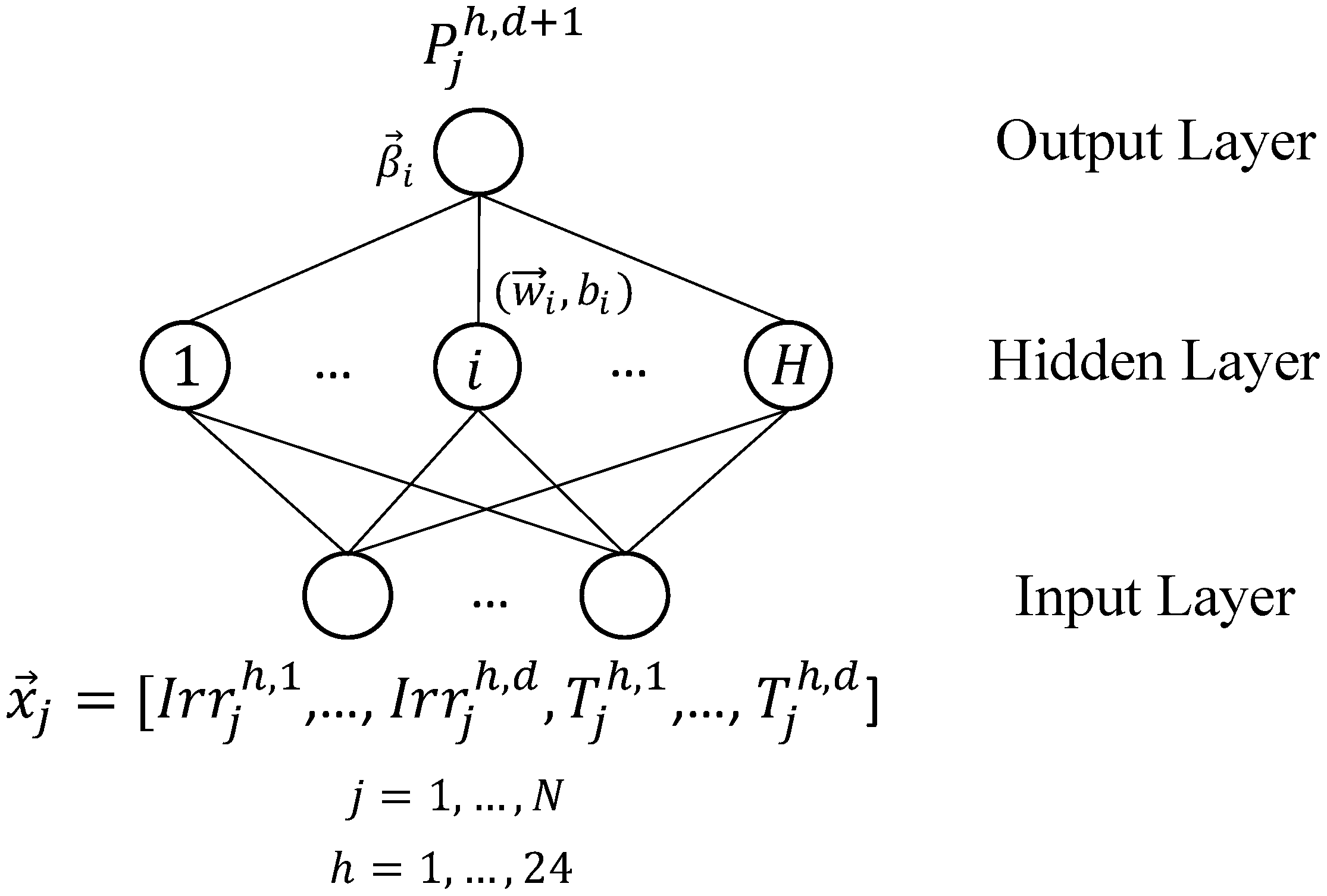
ELM is a new learning algorithm for single-hidden layer feedforward neural networks, originally developed by [34]. Figure 6 shows the architecture of ELM that consists of three layers (input, hidden and output layers):
- The input layer receives the -th pattern that comprises historical real radiation and ambient temperature values measured at hour in the past days, ;
- The hidden layer manipulates the inputs, it comprises hidden neurons (or nodes), via a neuron activation function, , that defines the output of each -th neuron (or node), , based on the received inputs;
- The output layer provides the -th solar PV power production value at the same time of the following day , , via the following equation (Equation (2)):
where is the weights vector that connects the inputs to each -th neuron, is the bias of each -th neuron, is the output weights vector that connects the outcomes of each -th neuron to the output node, and is the neuron activation function which is, in practice, a continuous non-polynomial function [34].
In simple words, the built-ELM should provide in output the prediction of the solar PV power production at time of the following day (i.e., one day ahead), , for an input pattern that comprises the historical real radiation and ambient temperature values measured at hour in the past days (as depicted in Figure 6).
The idea underpinning the operation of the ELM is that it randomly chooses the input weights, , and biases, , of each -th hidden neuron, , and analytically determines the output weights, by considering the pair of () inputs/output patterns as a training data, training patterns (for more details on the ELM, the interested readers may refer to [34]). Therefore, compared to the traditional BP-ANN that employs an iterative BP algorithm for setting the input weights and biases, ELM has been shown capable in providing better generalization performances with lower computational efforts necessary to train the ELM model [34,38].
4.1. Optimum Architecture of ELM Model
In this Section, the architecture of the ELM model is optimized in terms of (1) number of hidden neurons, ; (2) neuron activation function, , and (3) embedding dimension , to provide accurate 24 h-ahead predictions of the solar PV power productions on the validation dataset, . To this aim, we follow an exhaustive search procedure by considering:
- Nine possible numbers of hidden neurons, 10, 50, 100, 200, 300, 500, 700, 900, 1000;
- Five possible nonlinear piecewise continuous activation functions, “Sigmoid”, “Triangular Basis”, “Sine”, “Hard Limit”, and “Radial Basis” functions due to their wide used in literature (for more details on the neuron activation functions in ELM, the interested reader can refer to [39]);
- Five possible embedding dimensions, = 2, 4, 6, 8, 10, 12, 14.
The effectiveness of each ELM candidate architecture, i.e., characterized by any combination of the above-mentioned choices, is evaluated by quantifying the accuracy of the obtained predictions of the validation dataset, , using the RMSE standard metric, i.e., RMSE is the average error of the solar PV power production predictions (small RMSE values entail more accurate predictions). It is defined by (Equation (3)):
where and are the predicted and the true solar PV power productions, respectively, of each -th validation pattern, .
Specifically, a 10-fold Cross-Validation (CV) procedure is carried out to robustly evaluate the ELM prediction performance in terms of the RMSE: the training and validation patterns are sampled randomly from the 2015–2016 years data with a fraction of 60% (i.e., patterns) and 40% (i.e., patterns), respectively. The CV procedure is then, repeated 10 times (10-fold), using different patterns for training and validation datasets. The final RMSE value is then, calculated by averaging the 10 RMSE values of the 10 different simulations.
Table 1 reports the modelling parameters of the optimum ELM architecture found at the smallest RMSE value, i.e., RMSE = 13.4832 kW.
For clarification purposes, Figure 7 shows the performance of different ELM model architectures (i.e., average RMSE). Figure 7 (left) shows the influence of the neuron activation function, , on the final RMSE value, considering different numbers of hidden neurons, , when the embedding dimension, , is set to . One can easily recognize that:
- “Sine” and “Radial basis” neuron activation functions (circle and star markers, respectively) clearly outperform the Sigmoidal and Hard limit activation functions (square and diamond markers, respectively) and slightly outperform the “Triangular basis” activation function (triangle marker);
- As long as the number of hidden neurons, , increases, the prediction performance increases, i.e., the RMSE value decreases. This is justified by the fact that ELMs characterized by large hidden layers will have a better generalization capability and, hence, better prediction performances can be obtained [38,40]. However, for large number of neurons, i.e., , the prediction performance seems to be slightly stable and further increment in the number of neurons might not be necessary, as the computational efforts will increase too. In this regard, the best number of neurons is considered at (RMSE 13.4832 kW) obtained by the “Radial basis” neuron activation function.
Figure 7 (right) shows the influence of the numbers of hidden neurons, , considering different embedding dimensions, , when the neuron activation function, = “Radial basis” is selected. One can also notice that:
- Small and large embedding dimensions, , are not desired, whereas the optimum is found at the intermediate value . This is can be justified by the fact that the small embedding dimensions entail benefiting from the previous few global solar radiation and ambient temperature values measured in the previous days, that might not be sufficient to accurately predict the solar power productions, and vice versa: large embedding dimensions entail using the previous large global solar radiation and ambient temperature values measured in the previous days, that might be less correlated and, thus, less accurate predictions are obtained;
It is worth mentioning that this result is in line with the preventive maintenance program established for the PV system at the ASU campus concerning the cleaning of the PV panels. As a result, of, the soiling issue in the Jordanian dusty environment, which reduces the PV power production, and might lead to a localized hotspot failure when the soiling is uneven [41].
- Small number of hidden neurons, (square markers), is not able to accurately represent the solar radiation-power relationship, whereas large number of neurons is more favorable. In fact, in line with Figure 7 (left), further increment in number of neurons might not be necessary, as the computational efforts will be increased as well.
Here, the computational time needed to optimize the ELM model on an Intel Core i7 with 10-fold CV, equals to 6.8758 min. This provides insights on the time-effectiveness that can be achieved using the ELM, in particular, when the frequency of model updating, each time new solar radiation and ambient temperature-power values become available, is high.
4.2. Application Results of ELM Model
Once the optimum ELM architecture has been defined, it has been applied on the test dataset, , and its performance is evaluated on the test patterns by considering the RMSE (Equation (3)), the MAE and the WMAE performance metrics [42,43], using 10-fold CV:
- MAE: it is defined as the average error of the solar PV power production prediction. Smaller MAE values indicate more accurate predictions. MAE is defined by (Equation (4)):
- WMAE: it computes the average relative error. Smaller WMAE values indicate more accurate predictions. WMAE is defined by (Equation (5)):
where and are the predicted and the true solar PV power productions, respectively, of each -th test pattern, .
Table 3 reports the average performance metrics and their standard deviations over the 10-fold CV obtained by the application of the proposed ELM model, along with the time required for building the ELM model.
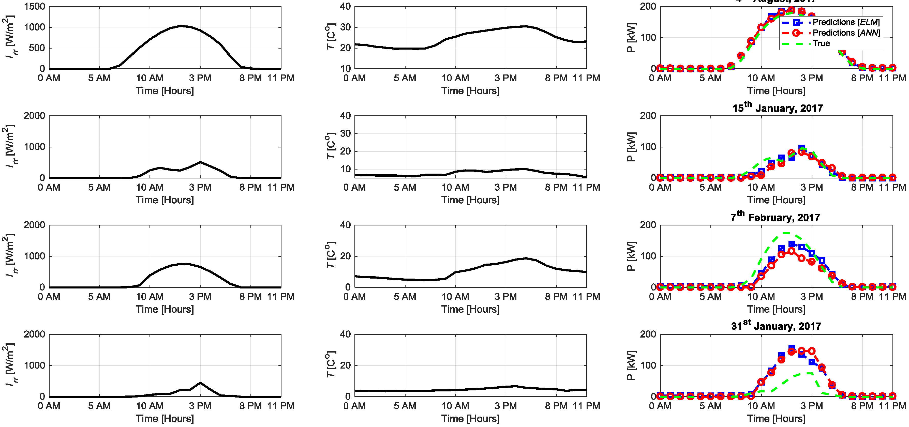
For clarification purposes, Figure 8 shows the global solar radiations (left), the ambient temperatures (middle), and the associated power production predictions (right) obtained by the proposed ELM model for four different days in 2017 representative of two different weather conditions, i.e., normal and anomalous: Figure 8 (top) shows an example of a sunny day characterized by a clear sky (4 August 2017); Figure 8 (top middle) shows an example of a cloudy day characterized by an extreme clouds sky (15 January 2017); Figure 8 (bottom middle) shows an example of haze day characterized by dust, smoke and dry particles that obscure the sky clarity (7 February 2017); Figure 8 (bottom) shows an example of a raining day characterized by raining and broken clouds (31 January 2017).
It can be seen that: (1) the predicted power productions are reasonably close to the true power productions (4 August), i.e., RMSE = 8.4046 kW; (2) due to the extreme weather conditions suffered by the ASU PV system (15 January, 7 February and 31 January), the ELM tends to provide over and under estimated (average) power predictions, i.e., RMSE = 9.6898, 22.4060 and 39.7119 kW, respectively. However, they are slightly better than those obtained by the BP-ANN model, as we shall see in Section 5.2; and (3) the predictions are, in general, more uncertain during the day hours (characterized by high solar radiations) than those of the early morning and late evening hours (characterized by low/no solar radiations). This is due to the large variability (stochasticity) of the global solar radiations and ambient temperatures during the day hours, as shown in Figure 5.
5. Comparison with ANN Prediction Model
In this Section, the data-driven BP-ANN [44,45] prediction model, has been applied to the solar PV case study and the obtained results are compared with those obtained by the proposed ELM model.
Inspired by the biological neural networks, ANN is a computational model comprises of several neurons (the computational units) directionally connected by weighted connections structured in a proper architecture that consists of three layers: input, hidden (with hidden neurons) and output layers [46]. Basically, ANN aims at capturing the underlying complex inputs/outputs, possibly nonlinear, relationships. The input layer receives the global solar radiation and ambient temperature values; the hidden layer processes the inputs via a neuron activation function, (Equation (2)), and send the manipulated information to the output layer for providing the solar power production value.
In this work, the motivation of selecting ANN for the comparison with the proposed ELMs (Section 4) is the fact that it has been adopted by the PV system owner and has provided accurate 24 h-ahead solar PV power productions predictions [31,32].
Unlike the ELM operation, the internal parameters (i.e., , and of the -th hidden neuron, ) of the ANN are defined by resorting to the iterative error BP algorithm in which the ANN model parameters are initially defined randomly, then updated in an iterative way by sampling the inputs-output from the training dataset, calculating the error on the outputs and distributing it back to the ANN model layers [44]. In this regard, setting the internal parameters of the ANN requires more computational efforts than those required by the ELM [38,44].
5.1. Optimum Architecture of ANN Model
Similar to the optimization procedure of the ELM architecture, the architecture of the ANN model is optimized in terms of (1) number of hidden neurons, ; (2) neuron activation function, ; and (3) embedding dimension, , for providing accurate 24 h-ahead predictions of the solar PV power productions on the validation dataset, . To this aim, we follow an exhaustive search procedure by considering:
- Six possible numbers of hidden neurons, = 1, 5, 10, 20, 40, 60, 90, 100, 110;
- Six possible nonlinear piecewise continuous activation functions, “Log-Sigmoid”, “Tan-Sigmoid”, “Linear”, “Triangular Basis”, “Radial Basis”, and “Elliot Symmetric Sigmoid” functions due to their wide used in literature (for more details on the neuron activation functions in ANN, the interested reader can refer to [47]);
- Five possible embedding dimensions, = 2, 4, 6, 8, 10, 12, 14.
The effectiveness of each ANN candidate architecture, i.e., characterized by any combination of the above-mentioned choices, is evaluated by quantifying the accuracy of the obtained predictions of the validation dataset, , using the RMSE metric (Equation (3)) over 10-fold cross-validation.
The modelling parameters of the optimum ANN architecture are found at using neuron activation function = “Log-Sigmoid” and solar radiation and ambient temperature values (Table 2). Notice that the developed BP-ANN architecture is characterized by slightly more number of inputs compared to that obtained for the proposed ELM model (i.e., ), with fewer hidden neurons (i.e., ) (Table 1) required to capture the solar radiation and ambient temperature-power relationship. However, with slightly less accurate predictions (i.e., RMSE = 14.2601 kW) than the best ELM model (i.e., RMSE = 13.4832 kW) when applied on the validation dataset, . In practice, the BP-ANN employs the BP algorithm that updates the weights and biases of the hidden neurons iteratively forward and backward, whereas the ELM is based on a one-time process that generates random weights and obtains the output weights analytically [34]. Consequently, fewer hidden neurons are required for the convergence of the ANN than the ELM model.
Although the number of hidden neurons in ANN is much less than those in ELM for an accurate solar power production prediction, the optimization of the ANN using 10-fold CV necessitates 129.4622 min, which is 18 times larger than the 6.8758 min required for the ELM architecture optimization of Section 3.2, due to the BP algorithm.
5.2. Application Results of ANN Model
To effectively compare the developed ANN model to that of the ELM, it has been applied on the test dataset, , and its performance is evaluated on the test patterns by considering the three previously defined performance metrics, using 10-fold CV.
Table 3 reports the average performance metrics and their standard deviations over the 10-fold CV obtained by the application of the developed ANN, along with the time required for building/training the ANN model, with respect to those obtained by the proposed ELM model. The performance gain () [48] of the ELM model with respect to the ANN model is calculated for the considered metrics, using:
Results show that the ELM model slightly enhances the accuracy of the solar power production predictions with respect to the use of the BP-ANN model (3%, 3.7% and 3.2% performance gains obtained for the RMSE, MAE and WMAE, respectively). It is worth mentioning that despite that these improvements in the prediction accuracy are relatively small, but they have been considered relevant to the PV system owner. Additionally, the short training times of the both models increase their potentiality in real time applications. In fact, large computational efforts are required for building the BP-ANN model than those required for building the ELM model (i.e., BP-ANN requires computational efforts by 106 times larger than those required by the ELM with enhancement reaches to 99%), due to the complex BP algorithm employed in the ANN model to effectively capture the solar radiation and ambient temperature-power relationship. This would be even more noticeable when:
- Large historical datasets are available for training the prediction models;
- High number of weather variables (e.g., humidity, wind speed, etc.) are available that might have an influence on the PV power productions. This would necessitate the selection of the most representative variables for accurate production predictions (feature selection);
- Several base prediction models must be, individually, trained within an ensemble whose outcome is the aggregation of the predictions obtained by the base prediction models, and/or
- The prediction models are required to be updated each period when new solar radiation-power values become available or when the context (environment) in which the plant is working changes (evolves). The former entails the availability of additional training patterns that can be exploited by the prediction models for enhancing their prediction accuracy, whereas the latter entails the presence of an evolving environment for which the existing prediction models need to be informed and updated for adapting to the new “not seen” weather conditions.
Examples of the 24 h-ahead solar power predictions obtained by the BP-ANN for four different days in 2017 representative of two different weather conditions, i.e., normal and anomalous, are shown in Figure 8 in circles (together with those obtained by the ELM model of Section 4.2 in squares). The predictions provided by the two approaches are comparable: the ELM provides accurate productions predictions in the four days than those obtained by the BP-ANN model, i.e., RMSE = 8.5202, 14.2107, 31.9605 and 39.8360 kW (compared to 8.4046, 9.6898, 22.4060 and 39.7119 kW obtained by the ELM), respectively. In particular, during the days’ hours, that is of paramount importance for the PV system owner.
For completeness, the prediction performances of the ELM model and the BP-ANN model are further evaluated by computing the average values of the three performance metrics for the months of 2017-year test dataset (Table 4). One can easily recognize that the ELM model outperforms the BP-ANN for most of the 2017-year months.
All these findings highlight the effectiveness of the ELM model with respect to the current BP-ANN model and suggest its development for the 24 h-ahead solar power production predictions at the ASU solar system.
6. Conclusions
In this work, we investigate the capability of a new learning algorithm for single-hidden layer feedforward neural networks, the ELMs, for the prediction of power production in solar photovoltaic system of a capacity of 264 kWp installed on the roof of the Faculty of Engineering at ASU, Amman, Jordan. Thanks to the simplicity, fast computational and good generalization capability of ELM, it has been shown capable of providing slightly accurate 24 h-ahead solar power productions with no computational constraints with respect to the BP-ANN, currently adopted by the ASU PV system owner for the prediction task.
Thus, the ELM-based model can be attractive for the development of empirical, data-driven models capable of providing as accurate as possible solar PV power productions predictions with negligible computational efforts. As mentioned previously, in practice, this would be even more appreciated when (i) large historical datasets are available; (ii) huge numbers of weather variables are available; (iii) ensemble approaches are needed to be developed to further enhance the production predictions; and (iv) context change has been detected. These could be objects for future research works. In addition, the investigations of other data-driven techniques, e.g., SVMs, and their comparisons for 24 h-ahead solar PV power productions predictions task could be of interest to provide the ASU solar PV system owners with guidelines for their deployment in practice.
Author Contributions
In this research activity, S.A.-D. was involved in the data analysis and preprocessing phase, simulation, results analysis and discussion, and manuscript preparation. O.A. and J.A. were involved in preprocessing phase, and manuscript preparation. M.A. and B.R.Q. were involved in manuscript preparation. All authors have approved the submitted manuscript.
Funding
This research received no external funding.
Acknowledgments
The authors would like to acknowledge the Renewable Energy Center at the Applied Science Private University for sharing with us the Solar PV system data. The authors would like to thank all the reviewers for their valuable comments to improve the quality of this paper.
Conflicts of Interest
The authors declare no conflict of interest.
Abbreviations
The following notations are used in this manuscript:
| Acronyms | |
| RE | Renewable Energy |
| TNSP | Transmission Network Service Provider |
| NEPCO | National Electric Power Company |
| JEPCO | Jordan Electric Power Company |
| IDECO | Irbid District Electricity Company |
| EDCO | Electricity Distribution Company |
| PV | Photovoltaic |
| ML | Machine Learning |
| BP-ANNs | Back Propagation Artificial Neural Networks |
| AI | Artificial Intelligence |
| WT | Wavelet Transform |
| RBFNN | Radial Basis Function Neural Network |
| SARIMA | Seasonal Auto-Regressive Integrated Moving Average |
| SVMs | Support Vector Machines |
| NWP | Numerical Weather Prediction |
| PSO | Particle Swarm Optimization |
| ELMs | Extreme Learning Machines |
| ASU | Applied Science Private University |
| Notations | |
| Weather variables | |
| Solar PV power productions | |
| Measurements time step | |
| Global solar radiation (W/m2) | |
| Ambient temperature at 1 m altitude (°C) | |
| Solar power production (kW) | |
| Minimum solar radiation value | |
| Maximum solar radiation value | |
| Normalized solar radiation value | |
| Minimum temperature value | |
| Maximum temperature value | |
| Normalized temperature value | |
| Minimum solar power value | |
| Maximum solar power value | |
| Normalized solar power value | |
| Training dataset matrix | |
| Validation dataset matrix | |
| Test dataset matrix | |
| Number of patterns used for training | |
| Number of patterns used for validation | |
| Number of patterns used for testing | |
| Number of available patterns used for training, validation, and testing | |
| Index of pattern, | |
| Number of ELM/ANN hidden neurons | |
| Index of number of hidden neuron, | |
| Index of hour, | |
| Embedding dimension (number of historical days) | |
| Solar radiation value of the -th pattern, at the -th measurement time of the day 1 | |
| Ambient temperature value of the -th pattern, at the -th measurement time of the day 1 | |
| Solar power production value of the -th pattern, at the -th measurement time of the day | |
| The input-hidden weight vector of the -th neuron, | |
| The hidden -output weight vector of the -th neuron, | |
| The bias of the -th neuron, | |
| ELM/ANN neuron activation function | |
| Cross-Validation procedure | |
| Root Mean Square Error | |
| Mean Absolute Error | |
| Weighted Mean Absolute Error | |
| True power production of the -th pattern | |
| Predicted power production of the -th pattern | |
| Performance gain of a Metric | |
References
- Ministry of Energy & Mineral Resources (MEMR). Annual Report 2015. Available online: http://www.memr.gov.jo/echobusv3.0/SystemAssets/6df2053d-ee21-4fa0-ada8-613049ab7015.pdf (accessed on 10 October 2018).
- National Electric Power Company (NEPCO). Annual Report 2015. Available online: http://www.nepco.com.jo/store/docs/web/2015_en.pdf (accessed on 10 October 2018).
- Department of Statistics. Jordan in Figures 2017. Available online: http://dosweb.dos.gov.jo/DataBank/JordanInFigures/JORINFIGDetails2017.pdf (accessed on 11 October 2018).
- Jaber, J.O.; Badran, O.O.; Abu-Shikhah, N. Sustainable Energy and Environmental Impact: Role of Renewables as Clean and Secure Source of Energy for the 21st Century in Jordan. Clean Technol. Environ. Policy 2004, 6, 174–186. [Google Scholar] [CrossRef]
- Al-omary, M.; Kaltschmitt, M.; Becker, C. Electricity System in Jordan: Status & Prospects. Renew. Sustain. Energy Rev. 2018, 81, 2398–2409. [Google Scholar]
- Ministry of Planning and International Cooperation. Jordan 2025 A National Vision and Strategy. Available online: http://www.nationalplanningcycles.org/sites/default/files/planning_cycle_repository/jordan/jo2025part1.pdf (accessed on 10 October 2018).
- Ministry of Energy & Mineral Resources (MEMR). Updated Master Strategy of Energy Sector in Jordan for the Period 2007–2020. Available online: http://eis.memr.gov.jo/publication/policy/law-policies/283-energy-strategy (accessed on 10 October 2018).
- Al Omari, A.; Ayadi, O. Integrating Solar PV with the Electricity Grid through Conventional Power Plants. In Proceedings of the 2017 8th International Renewable Energy Congress, IREC 2017, Amman, Jordan, 21–23 March 2017. [Google Scholar]
- Azzam, S.; Feilat, E.; Al-Salaymeh, A. Impact of Connecting Renewable Energy Plants on the Capacity and Voltage Stability of the National Grid of Jordan. In Proceedings of the 2017 8th International Renewable Energy Congress, IREC 2017, Amman, Jordan, 21–23 March 2017. [Google Scholar]
- Ayadi, O.; Alsalhen, I. Techno-Economic Assessment of Concentrating Solar Power and Wind Hybridization in Jordan. J. Ecol. Eng. 2018, 19, 16–23. [Google Scholar] [CrossRef] [Green Version]
- National Electric Power Company (NEPCO). Annual Report 2017. Available online: http://www.nepco.com.jo/store/docs/web/2017_en.pdf (accessed on 10 October 2018).
- Abul-Failat, Y. The Jordanian Electricity Market—A Transitory Regime. Oil Gas Energy Law Electr. Law Regul. 2013, 5. [Google Scholar] [CrossRef]
- Hudson, R.; Heilscher, G. PV Grid Integration—System Management Issues and Utility Concerns. Energy Procedia 2012, 25, 82–92. [Google Scholar] [CrossRef]
- Dinter, F.; Gonzalez, D.M. Operability, Reliability and Economic Benefits of CSP with Thermal Energy Storage: First Year of Operation of ANDASOL 3. Energy Procedia 2013, 49, 2472–2481. [Google Scholar] [CrossRef]
- Katiraei, F.; Aguero, J.R. Solar PV Integration Challenges. IEEE Power Energy Mag. 2011, 9, 62–71. [Google Scholar] [CrossRef]
- Von Appen, J.; Braun, M.; Stetz, T.; Diwold, K.; Geibel, D. Time in the Sun: The Challenge of High PV Penetration in the German Electric Grid. IEEE Power Energy Mag. 2013, 11, 55–64. [Google Scholar] [CrossRef]
- Jones, L. Renewable Energy Integration; Academic Press: Massachusetts, CA, USA, 2014; Available online: https://www.elsevier.com/books/renewable-energy-integration/jones/978-0-12-407910-6 (accessed on 10 October 2018).
- Burgholzer, B.; Auer, H. Cost/Benefit Analysis of Transmission Grid Expansion to Enable Further Integration of Renewable Electricity Generation in Austria. Renew. Energy 2016, 97, 189–196. [Google Scholar] [CrossRef]
- Das, U.K.; Tey, K.S.; Seyedmahmoudian, M.; Mekhilef, S.; Idris, M.Y.I.; Van Deventer, W.; Horan, B.; Stojcevski, A. Forecasting of Photovoltaic Power Generation and Model Optimization: A Review. Renew. Sustain. Energy Rev. 2018, 81, 912–928. [Google Scholar] [CrossRef]
- Dolara, A.; Grimaccia, F.; Leva, S.; Mussetta, M.; Ogliari, E. A Physical Hybrid Artificial Neural Network for Short Term Forecasting of PV Plant Power Output. Energies 2015, 8, 1138–1153. [Google Scholar] [CrossRef] [Green Version]
- Ernst, B.; Reyer, F.; Vanzetta, J. Wind Power and Photovoltaic Prediction Tools for Balancing and Grid Operation. In Proceedings of the CIGRE/IEEE PES Joint Symposium Integration of Wide-Scale Renewable Resources Into the Power Delivery System, Calgary, AB, Canada, 29–31 July 2009; pp. 1–9. [Google Scholar]
- Wan, C.; Zhao, J.; Member, S.; Song, Y. Photovoltaic and Solar Power Forecasting for Smart Grid Energy Management. J. Power Energy Syst. 2015, 1, 38–46. [Google Scholar] [CrossRef]
- Monteiro, C.; Fernandez-Jimenez, L.A.; Ramirez-Rosado, I.J.; Muñoz-Jimenez, A.; Lara-Santillan, P.M. Short-Term Forecasting Models for Photovoltaic Plants: Analytical versus Soft-Computing Techniques. Math. Probl. Eng. 2013, 2013, 767284. [Google Scholar] [CrossRef]
- Bacher, P.; Madsen, H.; Nielsen, H.A. Online Short-Term Solar Power Forecasting. Sol. Energy 2009, 83, 1772–1783. [Google Scholar] [CrossRef] [Green Version]
- Chow, S.K.H.; Lee, E.W.M.; Li, D.H.W. Short-Term Prediction of Photovoltaic Energy Generation by Intelligent Approach. Energy Build. 2012, 55, 660–667. [Google Scholar] [CrossRef]
- Omar, M.; Dolara, A.; Magistrati, G.; Mussetta, M.; Ogliari, E.; Viola, F. Day-Ahead Forecasting for Photovoltaic Power Using Artificial Neural Networks Ensembles. In Proceedings of the 2016 IEEE International Conference on Renewable Energy Research and Applications, ICRERA 2016, Birmingham, UK, 20–23 November 2016; pp. 1152–1157. [Google Scholar]
- Ding, M.; Wang, L.; Bi, R. An ANN-Based Approach for Forecasting the Power Output of Photovoltaic System. Procedia Environ. Sci. 2011, 11, 1308–1315. [Google Scholar] [CrossRef]
- Mandal, P.; Madhira, S.T.S.; Ul haque, A.; Meng, J.; Pineda, R.L. Forecasting Power Output of Solar Photovoltaic System Using Wavelet Transform and Artificial Intelligence Techniques. Procedia Comput. Sci. 2012, 12, 332–337. [Google Scholar] [CrossRef]
- Bouzerdoum, M.; Mellit, A.; Massi Pavan, A. A Hybrid Model (SARIMA-SVM) for Short-Term Power Forecasting of a Small-Scale Grid-Connected Photovoltaic Plant. Sol. Energy 2013, 98, 226–235. [Google Scholar] [CrossRef]
- Fernandez-Jimenez, L.A.; Muñoz-Jimenez, A.; Falces, A.; Mendoza-Villena, M.; Garcia-Garrido, E.; Lara-Santillan, P.M.; Zorzano-Alba, E.; Zorzano-Santamaria, P.J. Short-Term Power Forecasting System for Photovoltaic Plants. Renew. Energy 2012, 44, 311–317. [Google Scholar] [CrossRef]
- Alomari, M.H.; Adeeb, J.; Younis, O. Solar Photovoltaic Power Forecasting in Jordan Using Artificial Neural Networks. Int. J. Electr. Comput. Eng. 2018, 8, 497. [Google Scholar] [CrossRef]
- Alomari, M.H.; Younis, O.; Hayajneh, S.M.A. A Predictive Model for Solar Photovoltaic Power Using the Levenberg-Marquardt and Bayesian Regularization Algorithms and Real-Time Weather Data. J. Adv. Comput. Sci. Appl. 2018, 9, 347–353. [Google Scholar]
- Behera, M.K.; Majumder, I.; Nayak, N. Solar Photovoltaic Power Forecasting Using Optimized Modified Extreme Learning Machine Technique. Eng. Sci. Technol. Int. J. 2018, 21, 428–438. [Google Scholar] [CrossRef]
- Huang, G.-B.; Zhu, Q.; Siew, C. Extreme Learning Machine: Theory and Applications. Neurocomputing 2006, 70, 489–501. [Google Scholar] [CrossRef]
- Applied Science Private University (ASU). PV System ASU09: Faculty of Engineering. Available online: http://energy.asu.edu.jo/ (accessed on 10 October 2018).
- Das, K.U.; Tey, S.K.; Seyedmahmoudian, M.; Idna Idris, Y.M.; Mekhilef, S.; Horan, B.; Stojcevski, A. SVR-Based Model to Forecast PV Power Generation under Different Weather Conditions. Energies 2017, 10, 876. [Google Scholar] [CrossRef]
- Google Maps. Applied Science Private University, Al Arab St, Amman. Available online: https://goo.gl/qA4h3w (accessed on 27 September 2018).
- Yang, Z.; Baraldi, P.; Zio, E. A Comparison between Extreme Learning Machine and Artificial Neural Network for Remaining Useful Life Prediction. In Proceedings of the 2016 Prognostics and System Health Management Conference (PHM-Chengdu), Chengdu, China, 19–21 October 2016; pp. 1–7. [Google Scholar]
- Huang, G.B.; Wang, D.H.; Lan, Y. Extreme Learning Machines: A Survey. Int. J. Mach. Learn. Cybern. 2011, 2, 107–122. [Google Scholar] [CrossRef]
- Lawrence, S.; Giles, C.L.; Tsoi, A.C. What Size Neural Network Gives Optimal Generalization? Convergence Properties of Backpropagation. Networks 1996, 1–37. Available online: https://clgiles.ist.psu.edu/papers/UMD-CS-TR-3617.what.size.neural.net.to.use.pdf (accessed on 10 October 2018).
- Maghami, M.R.; Hizam, H.; Gomes, C.; Radzi, M.A.; Rezadad, M.I.; Hajighorbani, S. Power Loss Due to Soiling on Solar Panel: A Review. Renew. Sustain. Energy Rev. 2016, 59, 1307–1316. [Google Scholar] [CrossRef]
- Foley, A.M.; Leahy, P.G.; Marvuglia, A.; McKeogh, E.J. Current Methods and Advances in Forecasting of Wind Power Generation. Renew. Energy 2012, 37, 1–8. [Google Scholar] [CrossRef] [Green Version]
- Holttinen, H.; Miettinen, J.; Sillanpää, S. Wind Power Forecasting Accuracy and Uncertainty in Finland. Available online: https://www.vtt.fi/inf/pdf/technology/2013/T95.pdf (accessed on 10 October 2018).
- Rumelhart, D.E.; Hinton, G.E.; Williams, R.J. Learning Representations by Back-Propagating Errors. Nature 1986, 323, 533–536. [Google Scholar] [CrossRef]
- Hornik, K.; Stinchcombe, M.; White, H. Multilayer Feedforward Networks Are Universal Approximators. Neural Netw. 1989, 2, 359–366. [Google Scholar] [CrossRef]
- Muhammad Ehsan, R.; Simon, S.P.; Venkateswaran, P.R. Day-Ahead Forecasting of Solar Photovoltaic Output Power Using Multilayer Perceptron. Neural Comput. Appl. 2017, 28, 3981–3992. [Google Scholar] [CrossRef]
- Braspenning, P.J.; Thuijsman, F.; Weijters, A. Artificial Neural Networks: An Introduction to ANN Theory and Practice; Springer: Berlin/Heidelberg, Germany, 1995; Volume 931. [Google Scholar]
- Bonissone, P.P.; Xue, F.; Subbu, R. Fast Meta-Models for Local Fusion of Multiple Predictive Models. Appl. Soft Comput. J. 2011, 11, 1529–1539. [Google Scholar] [CrossRef]
Figure 1.
Electricity generation (GWh) and peak load (MW) for the period 2000–2016 (based on the data from [2]).
Figure 1.
Electricity generation (GWh) and peak load (MW) for the period 2000–2016 (based on the data from [2]).

Figure 2.
Share of Jordan installed generating capacity as on 20 June 2017 (based on the data from [11]).
Figure 2.
Share of Jordan installed generating capacity as on 20 June 2017 (based on the data from [11]).

Figure 3.
Jordanian market structure (single-buyer model) (simplified from [12]).
Figure 3.
Jordanian market structure (single-buyer model) (simplified from [12]).

Figure 4.
Weather station and PV system at ASU (retrieved and adapted from Google Maps [37]).
Figure 4.
Weather station and PV system at ASU (retrieved and adapted from Google Maps [37]).

Figure 5.
Hourly global solar radiations (top left), hourly ambient temperatures at 1 m altitude (top right) and corresponding solar power productions (bottom) in 2016.
Figure 5.
Hourly global solar radiations (top left), hourly ambient temperatures at 1 m altitude (top right) and corresponding solar power productions (bottom) in 2016.

Figure 6.
The Architecture of ELM model.

Figure 7.
Influence of the activation function vs. different numbers of hidden neurons (left) and influence of the numbers of hidden neurons considering different embedding dimensions (right) on the RMSE in ELM model.
Figure 7.
Influence of the activation function vs. different numbers of hidden neurons (left) and influence of the numbers of hidden neurons considering different embedding dimensions (right) on the RMSE in ELM model.

Figure 8.
Global solar radiations (left), temperatures (middle), and the associated power production predictions (right) obtained by the developed ANN model with respect to those obtained by the proposed ELM model for four different days in 2017.
Figure 8.
Global solar radiations (left), temperatures (middle), and the associated power production predictions (right) obtained by the developed ANN model with respect to those obtained by the proposed ELM model for four different days in 2017.


Table 1.
The modelling parameters of the optimum ELM architecture.
| RMSE (kW) | |||
|---|---|---|---|
| 300 | “Radial basis” | 10 | 13.4832 |
Table 2.
The modelling parameters of the optimum ANN architecture.
| RMSE (kW) | |||
|---|---|---|---|
| 60 | “Log-Sigmoid” | 12 | 14.2601 |
Table 3.
Average performance metrics and their standard deviations obtained by the developed BP-ANN model on the test dataset, with respect to the proposed ELM.
Table 3.
Average performance metrics and their standard deviations obtained by the developed BP-ANN model on the test dataset, with respect to the proposed ELM.
| Performance Metrics | BP-ANN () | ELM () |
|---|---|---|
| RMSE (kW) () | 15.53 ± 2.76 (0) | 15.07 ± 2.13 (2.98) |
| MAE (kW) () | 9.66 ± 1.86 (0) | 9.30 ± 1.41 (3.73) |
| WMAE () | 0.34 ± 0.06 (0) | 0.33 ± 0.04 (3.21) |
| Training Time (sec) | 37.14 ± 9.23 (0) | 0.35 ± 0.05 (99.07) |
Table 4.
Average performance metrics obtained by the developed BP-ANN model on the months of the test dataset, with respect to the proposed ELM.
Table 4.
Average performance metrics obtained by the developed BP-ANN model on the months of the test dataset, with respect to the proposed ELM.
| Month | ||||||
|---|---|---|---|---|---|---|
| BP-ANN | ELM | BP-ANN | ELM | BP-ANN | ELM | |
| January | 21.63 | 21.33 | 12.19 | 11.99 | 0.54 | 0.53 |
| February | 30.74 | 29.39 | 18.36 | 17.47 | 0.59 | 0.56 |
| March | 30.72 | 29.10 | 18.83 | 17.79 | 0.56 | 0.54 |
| April | 28.86 | 28.15 | 17.63 | 17.33 | 0.56 | 0.55 |
| May | 6.09 | 5.97 | 4.46 | 4.37 | 0.12 | 0.11 |
| June | 1.42 | 0.99 | 1.08 | 0.68 | 0.06 | 0.05 |
| July | 8.08 | 8.45 | 5.57 | 5.63 | 0.10 | 0.10 |
| August | 8.15 | 9.15 | 5.73 | 6.30 | 0.11 | 0.12 |
| September | 7.67 | 7.02 | 4.85 | 4.17 | 0.10 | 0.09 |
© 2018 by the authors. Licensee MDPI, Basel, Switzerland. This article is an open access article distributed under the terms and conditions of the Creative Commons Attribution (CC BY) license (http://creativecommons.org/licenses/by/4.0/).
Share and Cite
MDPI and ACS Style
Al-Dahidi, S.; Ayadi, O.; Adeeb, J.; Alrbai, M.; Qawasmeh, B.R. Extreme Learning Machines for Solar Photovoltaic Power Predictions. Energies 2018, 11, 2725. https://doi.org/10.3390/en11102725
AMA Style
Al-Dahidi S, Ayadi O, Adeeb J, Alrbai M, Qawasmeh BR. Extreme Learning Machines for Solar Photovoltaic Power Predictions. Energies. 2018; 11(10):2725. https://doi.org/10.3390/en11102725
Chicago/Turabian StyleAl-Dahidi, Sameer, Osama Ayadi, Jehad Adeeb, Mohammad Alrbai, and Bashar R. Qawasmeh. 2018. "Extreme Learning Machines for Solar Photovoltaic Power Predictions" Energies 11, no. 10: 2725. https://doi.org/10.3390/en11102725
Note that from the first issue of 2016, this journal uses article numbers instead of page numbers. See further details here.