Wind Turbine Wake Characterization for Improvement of the Ainslie Eddy Viscosity Wake Model


1
Department of Advanced Mechanical Engineering, Kangwon National University, Chuncheon-si 24341, Korea
2
Wind Energy Institute, Technical University of Munich, 85748 Munich, Germany
3
Division of Mechanical and Biomedical, Mechatronics and Materials Science and Engineering, Kangwon National University, Chuncheon-si 24341, Korea
*
Author to whom correspondence should be addressed.
Energies 2018, 11(10), 2823; https://doi.org/10.3390/en11102823
Submission received: 3 July 2018
/
Revised: 13 September 2018
/
Accepted: 11 October 2018
/
Published: 19 October 2018
(This article belongs to the Special Issue Solar and Wind Energy Forecasting)
Abstract
:This paper presents a modified version of the Ainslie eddy viscosity wake model and its accuracy by comparing it with selected exiting wake models and wind tunnel test results. The wind tunnel test was performed using a 1.9 m rotor diameter wind turbine model operating at a tip speed ratio similar to that of modern megawatt wind turbines. The control algorithms for blade pitch and generator torque used for below and above rated wind speed regions similar to those for multi-MW wind turbines were applied to the scaled wind turbine model. In order to characterize the influence of the wind turbine operating conditions on the wake, the wind turbine model was tested in both below and above rated wind speed regions at which the thrust coefficients of the rotor varied. The correction of the Ainslie eddy viscosity wake model was made by modifying the empirical equation of the original model using the wind tunnel test results with the Nelder-Mead simplex method for function minimization. The wake prediction accuracy of the modified wake model in terms of wind speed deficit was found to be improved by up to 6% compared to that of the original model. Comparisons with other existing wake models are also made in detail.
1. Introduction
Wind turbine rotors extract energy from wind that passes through them. This energy extraction makes changes in the wind flow so that the wind speed is reduced and the turbulence intensity is increased downstream. This phenomenon, known as the wind turbine wake, reduces the power production and increases the fatigue load of the downstream wind turbines [1,2]. Especially in a wind farm composed with many wind turbines, this wake effect generally reduces the power production efficiency of the wind farm by 10 to 20%, so it is common to optimize the layout of the wind farm to minimize the wake effect [1,3]. However, since further optimization of the wind farm layout is not possible after constructing a wind farm, the active control of the wake using blade pitching and nacelle yawing has been investigated recently [4,5,6,7,8,9,10].
The application of a wind farm control algorithm to an actual wind farm for verification is difficult to be realized, so most research on this topic is performed through simulation [4,5,6,7,8,9,10]. Also, high fidelity computational fluid dynamics (CFD) codes cannot be used for this purpose because of large computational loads, and therefore, simplified wind farm simulation codes including wind turbine dynamics and control are used [11].
The accuracy of the wake model in wind farm simulation codes is important because the performance of wind farm control is largely affected by the wind speed prediction from the wake model [12,13,14]. For this reason, many researchers are making efforts to verify the accuracy of the wake models and to improve it through wind tunnel tests or high fidelity numerical simulations. Wind tunnel tests and numerical simulations are very useful methods to develop new wake models or verify their accuracy because they can have a controlled flow environment repeatedly [15,16].
The wake model that can be implemented to wind farm simulation codes can be divided into two, the kinematic wake model and the field wake model [17]. The kinematic wake model, also known as the explicit model, basically predicts the wind speed deficit in the wake based on the momentum equation. The kinematic wake model also features a self-similar wind speed profile. The kinematic wake model is also widely used in research fields such as predicting the annual power production of wind farms or wind farm design because it is possible to predict the wake field very quickly through simple equations [4,5,6,7,8,9,10].
The kinematic wake models have limitations in that the effect of turbulent momentum change on the wake growth and expansion cannot be considered. Therefore, the kinematic wake models fill the physically missing parts with empirical wind speed profiles and other parameters that can take into account the turbulence effects [17]. The Jensen wake model is one of the oldest kinematic wake models and is still widely used. The Jensen wake model predicts the wake using an unrealistic wind speed profile called the ‘top hat’ and a wake decay constant which is the wake recovery rate parameter. However, a relatively recent study by Kim showed that the Jensen wake model is not less accurate than other classical kinematic wake models with more realistic wind speed profiles such as the wake models by Larsen or Frandsen [18,19,20]. The wake decay constant in the Jensen model is an empirical parameter used to consider the effect of the ambient turbulence intensity due to the surface roughness on the wake [21]. The original Jensen wake model was modified by Katic so that the wake behind a wind turbine with power regulation by stall or pitch could be calculated differently by considering the change in the thrust coefficient [18].
Several studies were carried out to construct a wake model with a higher accuracy while retaining the advantages of the kinematic wake model by correcting the wake decay constant or the wind speed profile [1,22,23,24,25,26]. Wind Atlas Analysis and Application Program (WAsP), and recommends using the empirically derived wake decay constants of 0.05 and 0.075 for onshore and offshore, respectively. However, Barthelmie and Jensen found that the power production of a wind farm can be changed due to the atmospheric conditions through the measurement in Nysted offshore wind farm. They also found that the wake decay constant of 0.03 is suitable for Nysted wind farm. This value is smaller than the wake decay constant proposed by WAsP for offshore [1]. Peña et al. proposed a new wake decay constant calculation formula that can take into account the atmospheric stability to increase the accuracy of the Jensen wake model [27]. However, they did not do enough to fully validate the proposed model [21]. Tian pointed out that the wake growth is greatly affected by the ambient turbulence intensity which is not considered in the Jensen model, and he proposed a new wake decay constant formula considering the effect of the atmospheric turbulence intensity. The proposed model, however, showed improved prediction compared to the original Jensen wake model only for the below rated wind speed region. The proposed wake model was found to have large errors for different thrust coefficients (above rated wind speed region).
Kinematic models have also been modified to be more accurate by combining momentum conservation with the data obtained from wind tunnel tests or numerical simulations. Bastankhah and Porté-Agel (BP) proposed a new kinematic wake model with a Gaussian wind profile using the data from Large Eddy Simulation (LES) model and verified it by LES simulations with various roughness lengths [28]. However, their wind turbine in the LES simulation was different from a typical megawatt class wind turbine in that the tip speed ratio was only between 3 and 4 which is significantly smaller than that of modern wind turbines, which are between 7 and 10 [29]. Also, the validation was made only for a single thrust coefficient at a fixed tip speed ratio corresponding to the below rated wind speed region.
Ishihara conducted a wind tunnel test using a 1/100 scale model of Mitsubishi’s MWT-1000 in 2004 and proposed a new wake model with a Gaussian wind profile by combining the measured wake data and the momentum conservation equation [25]. He constructed a wake model through the wind tunnel test using a scaled wind turbine with a rotor diameter of 57 cm considering variations of the thrust coefficient and the ambient turbulence intensity. However, since the blade pitch angle of the wind turbine model was fixed, the tip speed ratio of the model had to be adjusted to change the thrust coefficient to cover the wake in the above rated wind speed region. This operating condition is different from that of general modern megawatt class wind turbines with active pitching.
Unlike kinematic wake models, field wake models are implicit models that are based on time or space averaged Navier-Stokes equations. They yield the magnitude of the velocity over the entire flow field as a solution of the implicit equation [17]. Therefore, field wake models require more computing power than kinematic wake models. In recent years, the remarkable increase in computation speed has led many researchers to use computational fluid dynamics (CFD) to characterize the wake effect and develop wake reduction strategies [30]. The CFD-based wake analysis is known to provide high accuracy because the wind turbine rotor is modeled and the flow field around the rotor is calculated with Navier–Stokes equations [31]. The Energy Research Center of the Netherlands (ECN) developed a three dimensional wake model called WakeFarm based on the UPMWAKE proposed by Crespo et al. [24]. The basic background flow of UPMWAKE is known to be modeled by the atmospheric wind profile model based on the Monin-Obukhov similarity theory [32]. The initial WakeFarm used a hat-shaped initial wind profile similar to that of the Jensen wake model.
Schepers tried to improve the initial WakeFarm, in the Efficient Development of Offshore Wind Farms (ENDOW) project and proposed a Gaussian initial wind profile obtained from a wind tunnel test. He verified the model with the test data from the wind tunnel and from the field. Although the model was in good agreement with the measured data at the location where the initial profile was applied, the error increased with the downstream distance.
The Ainslie eddy viscosity wake model is one of the oldest field models and is a wake model based on parabolized Reynolds averaged Navier-Stokes (RANS) equations [33]. Ainslie simplified the equation by assuming axisymmetric flow and by ignoring the pressure gradient, and constructed a model that can be solved relatively quickly and accurately. However, this caused the disadvantage that the model cannot be applied to the region close to the rotor where the pressure gradient is dominant.
Unlike WakeFarm, the Ainslie eddy viscosity model uses two empirical models such as the initial wind speed profile and the filter function to reduce the error of the wake prediction. The two empirical models are derived from the wind tunnel tests that take into account the change of the thrust coefficient and the downstream distance [34]. However, since the wind turbine scale model used to construct the empirical wake model was not pitch regulated as the wind turbine model used by Ishihara, the tip speed ratio was adjusted to change the thrust coefficients of the wind turbine model.
In this study, a new wake model based on the Ainslie eddy viscosity wake model was investigated to improve the current weaknesses of the model. For this, a wind tunnel test was performed with a scaled wind turbine which has an active pitching mechanism similar to that of modern large capacity wind turbines.
Although research articles with a similar scope are available in the literature, the originality of this study can be summarized as follows. The first is the wind turbine scale model used in this study. It was simply a scaled wind turbine with pitch actuators. Therefore, the wake could be measured both below and above the rated wind speed regions to cover different thrust coefficients by pitching the blades. Adjusting the tip speed ratio in the below rated wind speed region only for wake measurement purposes was not implemented any more.
The second is the control of the scaled wind turbine. A Bachmann programmable logic controller (PLC) with torque and pitch control algorithms embedded was used as a controller for the scaled wind turbine. Therefore, the operating of the wind turbine while the wake was measured in the downstream of the turbine was very similar to that of modern large capacity wind turbines such as the maximum power point tracking in the below rated wind speed region and the closed loop power regulation not to exceed the rated value using a PI controller in the above rated wind speed region. The third is the modification of the initial wake profile and the filter function of the original the Ainslie eddy viscosity model to obtain a more accurate wake model that can be used for both below and above rated wind speed regions. To show the performance of the proposed wake model more clearly, the result was compared with those of the wake models proposed by other researchers having a similar scope.
2. Experimental Setup
2.1. Measurement Apparatus
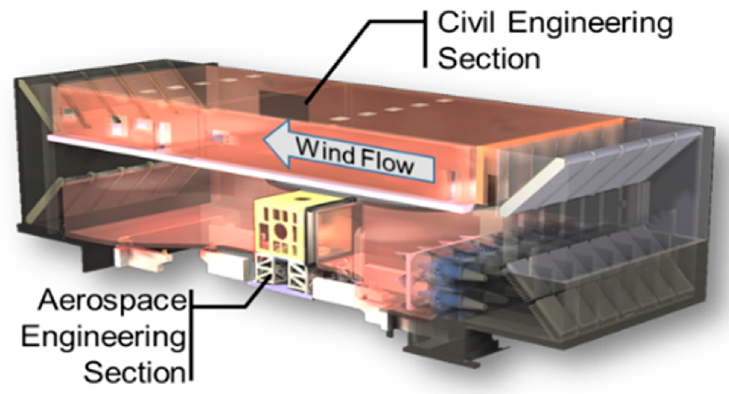
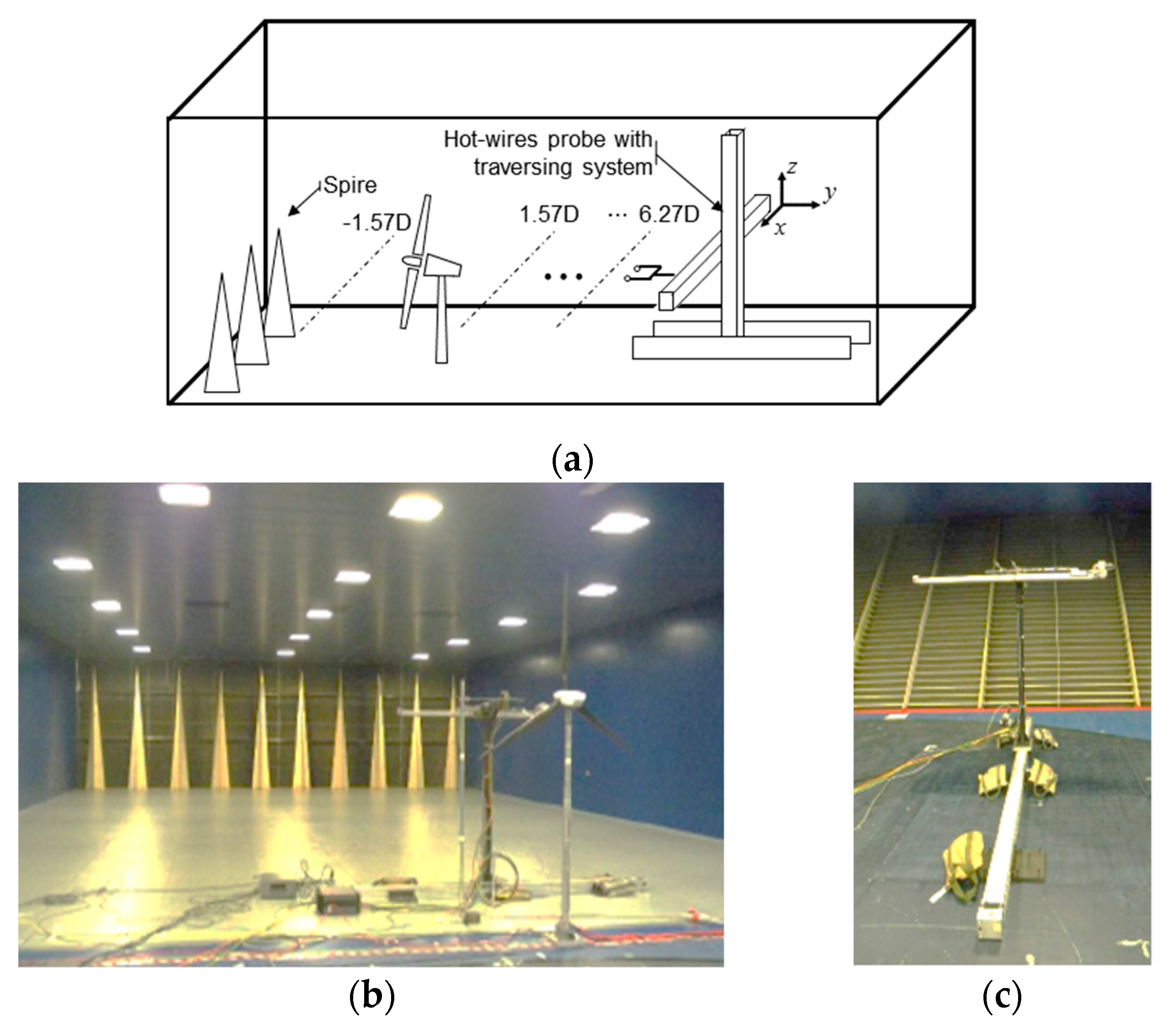
Wake measurements were carried out in a large closed-loop wind tunnel at the Technical University of Milano, as shown in Figure 1. The wind tunnel used for the wake measurement is divided into sections suitable for aerospace engineering (i.e., high wind speed with low turbulence) and civil engineering. This study was carried out in the civil engineering section, which generates wind up to 16 m/s. A spire installed near the inlet can implement an atmospheric boundary layer and generate a turbulence intensity of 2–35%. Generating an atmospheric boundary layer with a spire is a widely used method and has been verified by many studies [35]. The wind tunnel has a height, width, and length of 3.84, 13.84, and 36 m, respectively [36].
To consider the wake from a modern megawatt class wind turbine, the scaled wind model used was designed to have similar tip speed ratio, 7.5. The AH79100C and WM006 airfoils suitable for low Reynolds numbers were used for the scaled wind turbine model [37]. Figure 2 shows the comparison of the aerodynamic performances of the National Renewable Energy Laboratory (NREL) 5 MW wind turbine and the scaled model. All information of the NREL 5 MW wind turbine was taken from the literature [38]. As shown in Figure 2a, both blades have the maximum power coefficient (CP) at a similar tip speed ratio.
The rotor diameter of the scaled model is 1.91 m, and the rated power is 127.7 W at 5.8 m/s. The scaled wind turbine was designed to achieve the maximum power coefficient in the below rated wind speed region and to maintain the rated power in the above rated wind speed region by controlling the blade pitch angle and the generator torque. The control algorithms written in C codes were implemented to a PLC. Table 1 presents the details of the scaled model. The design and other details of the model are given by Bottasso [37]. The downstream wind speed of the scaled model was measured by using two three-directional DANTEC streamline hot-wire probes. The hot-wire probes were installed in reference to the height of the wind turbine hub and measured the wind speed only in the lateral direction with the same height.
2.2. Experimental Arrangement
The wake measurement was performed considering the changes of the wind turbine thrust coefficient and the downstream distance. The thrust coefficient of the wind turbine was changed by adjusting the input wind speed and the power control of the scaled model. The wind speeds of 5 m/s and 7 m/s were used to represent the below and above rated wind speed regions. Figure 3 shows the changes in the power and thrust coefficients according to the blade pitch adjustment.
As shown in Figure 3a, the scaled wind turbine used in the wind tunnel test has a blade pitch angle and a TSR that can keep the power coefficient close to its maximum value when the input wind speed is lower than the rated wind speed. Since the kinetic energy extraction of the wind is performed by obstructing the wind flow, the thrust coefficient becomes higher in the below rated wind speed region than that in the above rated wind speed region. On the other hand, when the wind speed is higher than the rated wind speed, the scaled wind turbine adjusts the pitch angle of the blade to maintain the rated power. This pitch angle adjustment reduces the aerodynamic efficiency of the blades, resulting in the reduction of power coefficient. The reduction in the power coefficient reduces the interference with the wind flow, and thereby reduces the thrust coefficient of the scaled wind turbine.
Figure 3b shows the changes in the thrust coefficient caused by the blade pitch angle adjustment. The result showed that the thrust coefficient was about 0.8 in the below rated wind speed region and 0.36 in the above rated wind speed region.
The input wind speed was measured with a hot-wire probe installed at 1.57 D (D; Rotor Diameter) ahead of the scaled wind turbine model. The wake was measured with an auto-traversing system after the distance was equally divided into 40 increments corresponding to ±1.5 D in the lateral direction. Figure 4a shows the experimental setup for the wind turbine wake measurements. Figure 4b,c show the actual wind tunnel test environment.
3. Wake Model
The wake is divided into the near- and far-wake regions according to the downstream distance [39]. In the near-wake region, which is about 2–3 D behind the wind turbine, the pressure gradient is dominant. In the far-wake region, the pressure gradient generated in the near-wake region disappears [17]. To know the accuracy of the wake models available in the literature, some of the wake models were used to simulate the far-wake region, and the results were compared with the measured wind profile. Four kinematic wake models and one field wake model were selected for the comparison. Each model and the governing equations are briefly described below.
3.1. Kinematic Wake Model
Kinematic wake models are based on relatively simple assumptions, such as the law of energy conservation. In this study, wake models by Jensen, Larsen, Bastannhah & Porté-Agel, and Ishihara were selected as representative kinematic wake models.
3.1.1. Jensen Wake Model
The first Jensen model was proposed in 1983 and simulates a wind turbine wake by using a wake decay constant that reflects the thrust coefficient and the effect of atmospheric turbulence intensity. The wake model calculates the wind velocity in the wake region as follows [18,19]:
where CT is the thrust coefficient, x is the distance in the downstream direction and α is the wake decay constant. The wake decay constant is used to determine the extent of the wake region expansion and wake speed which varies with the ambient turbulence intensity. In general, a value of 0.075 is applied to onshore turbines with a high ambient turbulence intensity, and 0.04 is applied to offshore turbines with a relatively low turbulence intensity. In this study, 0.04 was applied in consideration of the smooth bottom of the wind tunnel. The deficit Du is defined as follows:
where U0 is the input wind speed of the wind turbine. The Jensen model assumes that the wind speed decreases at the same rate as the wake region linearly increases with the downstream distance.
3.1.2. Larsen Wake Model
The Larsen wake model was proposed in 1988 and is based on the turbulent boundary layer equation. This model assumes a circular symmetric wake deficit by ignoring the pressure gradient based on the assumption of fluid incompressibility. The Larsen model uses two terms to calculate the downstream wind profile:
where w(x) is the weight of Du1 according to the distance. Du1 and Du2 can be calculated as follows: [40].
where r is the axial and radial indices, which are in units of D, and A is the rotor area. The wind turbine position x0 and Prandtl mixing length c1 can be calculated as follows:
where Deff is the effective rotor diameter and R9.5 is the wake radius at 9.5 times the rotor diameter downstream of the wind turbine. Each parameter can be calculated as follows:
Rnb is a parameter that empirically represents the blockage effect when the wake radius is greater than the wind turbine hub height [41].
3.1.3. Bastankhah and Porté-Agel Wake Model
Bastankhah and Porté-Agel (BP) proposed a new analytical wake mode in 2014. This wake model was constructed on the basis of a simplified momentum equation as the general analytical wake model and basically assumes the wind profile in the wake Gaussian shape [28]. The governing equation is shown in Equation (10),
where σ is the standard deviation of the Gaussian-like velocity deficit profiles at each x. C(x) is the maximum normalized velocity deficit at the wake center along the downstream location. C(x) is defined as Equation (11)
Also, the wake variation according to the ambient turbulence intensity can be calculated using the wake growth rate, k*, as shown in Equation (12).
Substituting Equations (11) and (12) into Equation (10), the final expression for the velocity deficit can be obtained.
where y and z are the lateral and vertical coordinate, respectively, and zh means the hub height.
3.1.4. Ishihara Wake Model
The Ishihara wake model was developed by wind tunnel test using a scaled model of Mitsubishi wind turbine in 2004. Although this wake model is based on the energy conservation laws like other analytical wake models, it has the advantage of using ambient turbulence intensity directly to calculate the wake width. The Governing equation of the Ishihara wake model is as follows [25].
where Uw is the wind speed in the wake and b is the wake width. The wake width, b, can be calculated using the following equation.
where p is the rate of wake recovery and is influenced by the turbulence intensity. p is defined by the following equation.
where Ia and Iw represent the ambient turbulence intensity and generated turbulence intensity by wind turbine, respectively. Iw can be calculated by Equation (17).
In Equations (14)–(17), k1–3 are parameters derived from the experiment and have values of 0.27, 6.0 and 0.004, respectively.
3.2. Field Wake Model
The Ainslie eddy viscosity wake model is a parabolic RANS model that is also called the boundary-layer wake model. It ignores the pressure gradient and assumes an axisymmetric wind profile [33]. The governing equation is as follows:
where is the Reynolds stress and is defined as follows:
Ainslie implemented the momentum transfer in the wake region by dividing ε in Equation (19) into two terms:
where εa is the ambient turbulence contribution to the eddy viscosity. Equation (20) can be calculated as follows:
where k1 is the dimensionless constant proposed by Ainslie, which is 0.015. KM is the eddy viscosity of momentum. Also, F is the filter function, which is a parameter used to simulate the effect of the eddy’s momentum on the wake region. It is applied differently according to distance:
Ainslie assumed that if the downstream distance is less than 5.5 times the rotor diameter, only some of the eddy momentum is recovered by the wind speed. On the other hand, when the downstream distance reaches 5.5 times the rotor diameter, all of the eddy momentum is assumed to be transferred to the wind speed recovery.
4. Results and Discussion
All of the wake data presented below were measured at a constant air density. Also, the proposed wind profile is the normalized result using the mean wind speed measured by hot-wire probes 1.57 D ahead of the wind turbine.
4.1. Comparison with the Wake Model
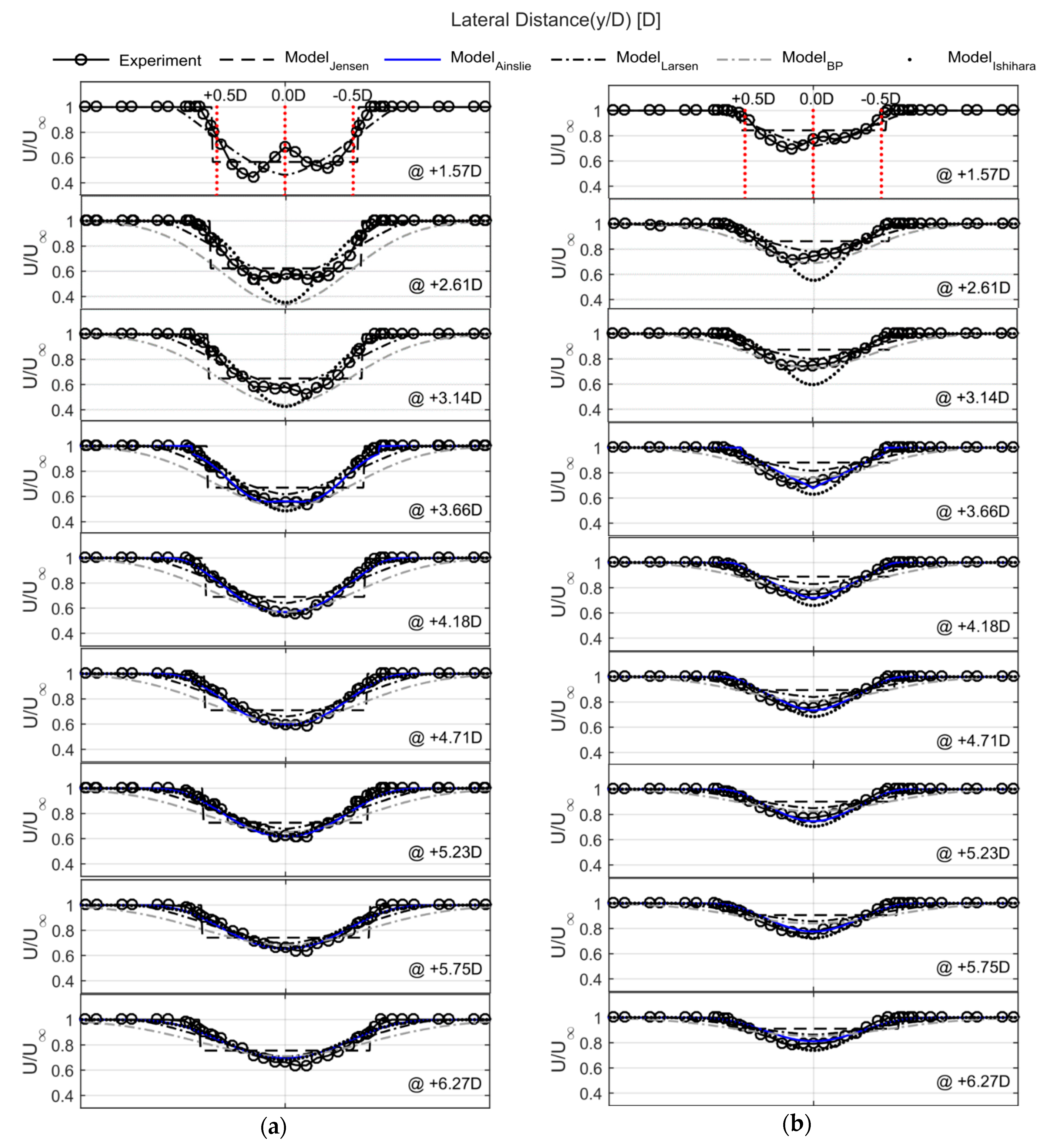
The wind profile changes in the wake region were measured at a fixed thrust coefficient of the wind turbine. Figure 5a shows the measured wake profile of the scaled wind turbine model operating at below rated wind speed and the comparison result of the predicted wake profiles through wake models. Figure 5b shows measured wake profile of the above rated wind speed case.
As shown in Figure 5a, the wind speed reduction due to the kinetic energy extraction was mainly centered at the mid-span (±0.25 D–0.3 D), which is critical for the aerodynamic performance of wind turbine blades [42]. The wind speed reduction decreased away from the mid-span. This phenomenon resulted in a double-dip wind speed reduction, which was observed up to 3–4 D. Thus, it had a relatively dominant effect on pressure gradient. As the downstream distance increased, the wind speed reduction profile became parabolic and eventually disappeared. Since the wake profile measured in this wind tunnel test was measured by moving the hot-wire probe, the meandering of the wake and the centerline offset were not clearly confirmed in the measured data.
As shown in Figure 5a, none of the wake models considered in this study could simulate the double-dip shape of the wake profile near the wind turbine rotor because they ignored the pressure gradient in the region close to the wind turbine. In particular, the Jensen wake model differed from the measured wind profile because it assumed the hat-shaped wind profile. However, other wake models which assumed a Gaussian wind profile such as the Larsen wake model, had profiles similar to the measured one in the far-wake region, where the pressure gradient disappeared.
The most remarkable point of this wind tunnel test is the accuracy of the wake model which uses the empirical model developed by a wind tunnel test or is developed through Large eddy simulation (LES) analysis. The Ainslie eddy viscosity wake model uses the empirical initial wake profile obtained from the wind tunnel test as mentioned above. The initial wake profile model is applied to the downstream 2 D, and then the wake calculation based on the parabolized RANS is performed. For this reason, it can be seen that the wake profile at the 2 D downstream from the turbine is very similar to the measured wake profile. However, the wake prediction accuracy of the Ainslie eddy viscosity wake model decreases gradually as the wake propagates downstream. This wake prediction error occurs because the Ainslie eddy viscosity wake model cannot sufficiently simulate the physical phenomena existing in the wake region.
The BP wake model based on the wind tunnel test and the LES analysis predicts the wind speed deficit at the wake center line very accurately. The BP wake model, however, showed a high accuracy only in the wake centerline, and overestimated the width of the wake. On the other hand, the Ishihara wake model developed through the wind tunnel test showed a very similar wake profile to the actual measured wake from 3.66 D, where the double dip phenomenon disappears. The Ishihara wake model showed very accurate prediction in the wake deficit at the wake center line as well as the wake width. On the other hand, if the thrust coefficient of the wind turbine is reduced as shown in Figure 5b, double dip phenomenon does not occur even if it is close to the region. In addition, it can be found that the wake width expansion and the wind speed recovery are similar to the below rated case in accordance with the increase in the downstream distance.
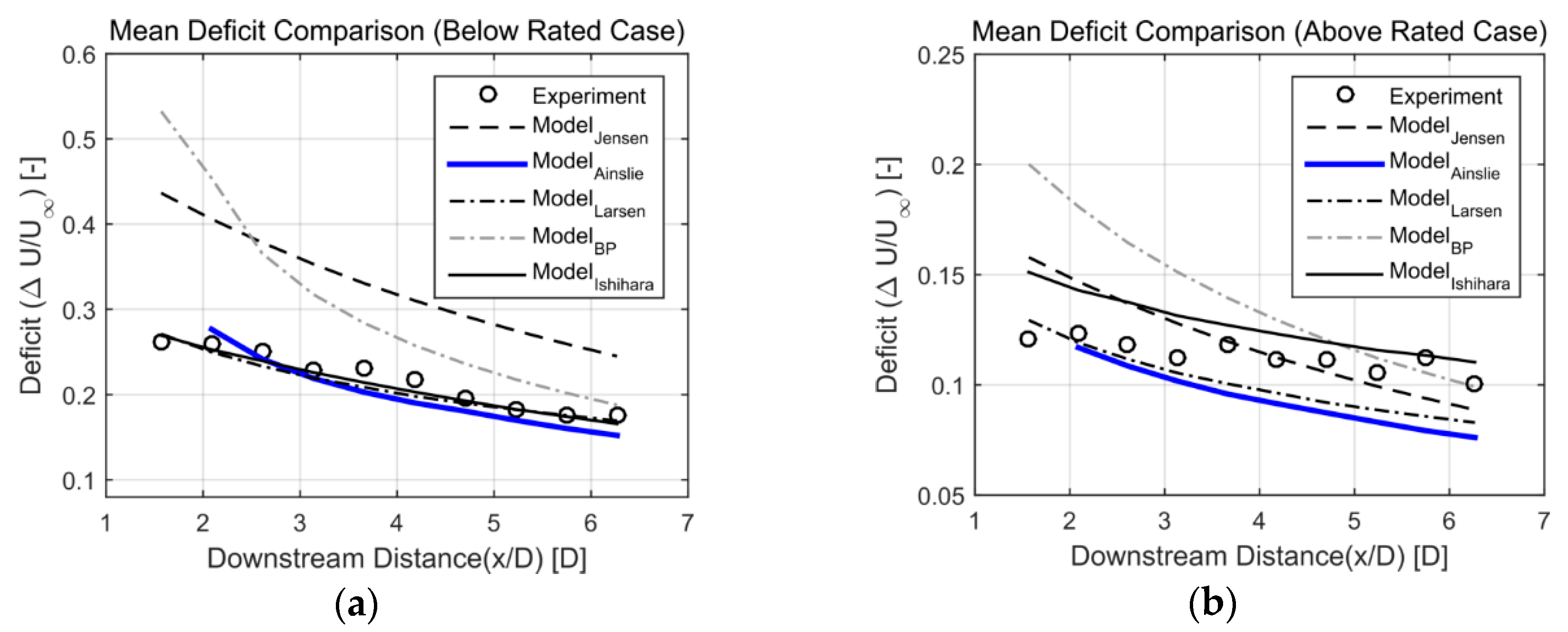
Figure 6 shows the comparison of the mean wind speed deficit from the wake models and the wind tunnel test. The mean deficit was calculated in the wake region bounded by U/U0 < 0.95 which is the boundary used to calculate the mean deficit in Parkin’s study [43].
As shown in Figure 6a, most of the wake models assuming the Gaussian wake, profile including the recently developed Ishihara wake model, predict the average wind speed deficit and recovery in the wake region and are very similar to the actual measured wake when input wind speed is lower than the rated wind speed. On the other hand, the Jensen wake model and the BP wake model predicted excessive wind speed deficit compared to the actually measured wake, as shown Figure 6a. The comparison results show that a wake model can improve its accuracy if it is developed or modified through full size wind turbine simulations or wind tunnel tests with scaled wind turbines.
Figure 6b shows the comparison of the measured wind speed deficit with the actual measured wake data when the input wind speed is higher than the rated wind speed. As shown in Figure 6a, most of the wake models considered in this study showed relatively high accuracy when the input wind speed was lower than the rated wind speed. However, if the thrust coefficient of the wind turbine changed, the accuracy of the wake prediction was decreased as shown in Figure 6b.
The Ainslie eddy viscosity wake model considered in this study uses the parabolized RANS and the empirical model at the same time to predict the wake, but it is not much different in the mean deficit errors from the other wake models. In particular, the error of the Ainslie eddy viscosity wake model was larger than that of the recently developed Ishihara wake model.
4.2. Wake Model Modification
The Ainslie eddy viscosity wake model calculates the wind speed variation in the wake region by using an initial profile, which is originally given by
where DM and b are calculated as follows:
where I0 is the ambient turbulence intensity in percentage. The original Ainslie eddy viscosity wake model uses Equation (23) to calculate the initial wind speed profile which is applied to 2 D downstream. In this study, the initial profile and filter function were modified based on the measured wake profile and the Nelder Mead simplex algorithm. The Nelder Mead simplex method is one of the function minimization algorithms used to find the parameters that can minimize the value of the objective function. The detailed operation principle of the algorithm can be found in the literature [44,45].
The objective function of the algorithm to calculate the initial wind speed profile is shown in Equation (26). The initial profile of the wake was calculated at 3.66 D behind the wind turbine, which is the location where the double dip shape in the wake profile disappeared:
In Equation (26), J is the objective function used in the function minimization algorithm, UExp3.66 is the measured wake profile at 3.66 D and UModel is the calculated wind profile. UModel can be obtained by Equation (27)
where P1–P6 are the dimensionless parameters obtained from the function minimization algorithm to match the actual wake profile. Table 2 shows the parameters obtained for the initial wake profile.
Similarly, the following objective function was used to construct the filter function:
Note that J in Equation (28) is the objective function used in the function minimization algorithm to calculate the parameters of the modified filter function. Note that it is not the same as Equation (26). J1 and J2 in Equation (28) can be calculated by Equations (29) and (30).
where δ is the wake width. The Ainslie eddy viscosity wake model does not have a separate formula for the wake width unlike the general analytical wake model, but the wake width can be modified by modifying Equation (22) which was derived from Ainslie’s wind tunnel test. Therefore, in this study, the filter function in Equation (22) was modified to be
where P1, P2, and P3 were found from the function minimization algorithm to match the actual wake profile. Table 3 presents the parameters obtained from the function minimization algorithm.
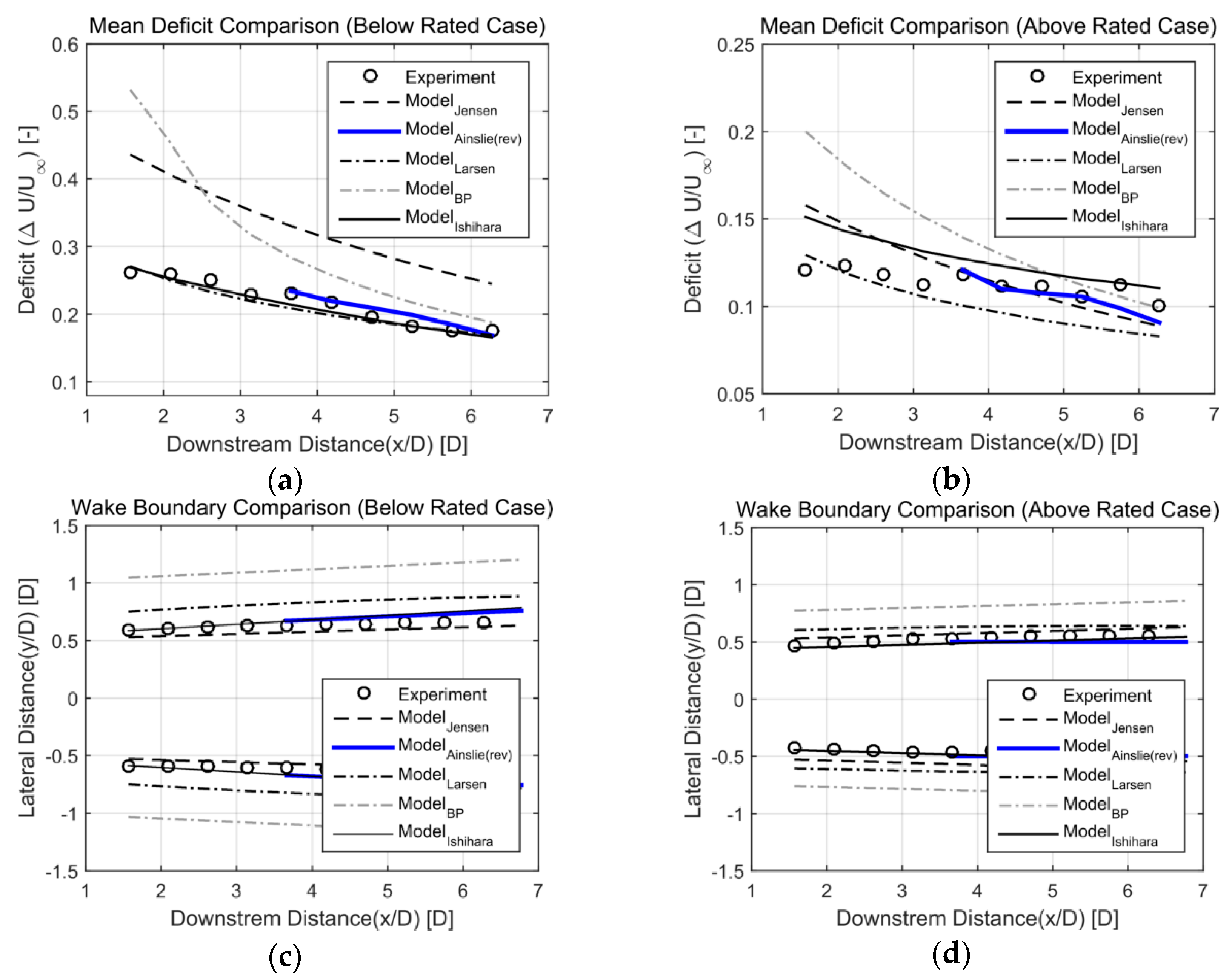
Figure 7 shows the comparison of the wakes measured by the wind tunnel test and predicted through the wake models. Figure 7 shows the wake prediction accuracy of the modified Ainslie eddy viscosity wake model with respect to the wind turbine thrust coefficient variation. Figure 7a,b shows the mean wind speed deficit in the wake region by distance for the below and above wind speed regions, respectively. As shown in Figure 7a, the modified Ainslie eddy viscosity wake model showed higher prediction accuracy than other classical kinematic wake models. In particular, the modified Ainslie eddy viscosity showed high accuracy not only at 3.66 D, which is the location where the empirical initial profile was applied, but also in the subsequent locations where the wake predictions were made based on the parabolized RANS. Figure 7b also shows that the modified Ainslie eddy viscosity wake model has high accuracy even when the thrust coefficient of the wind turbine is decreased.
As shown in Figure 8a,b, the Ainslie eddy viscosity wake model with the modified initial wind speed profile and the filter function predicted wakes very close to the measured wake data. In particular, the modified Ainslie eddy viscosity predicts the mean wind speed deficit very close to the actual measured wake data even when the thrust coefficient of the wind turbine changes (above rated wind speed region).
Figure 8c,d shows that the modified Ainslie eddy viscosity wake model improves the accuracy of the wake width as well as the wind speed mean deficit in the wake region. Figure 8c shows the predicted wake width for each wake model when the input wind speed is lower than the rated wind speed. As shown in the Figure 8, most of the wake models have a wider wake region than the actual wake width. However, the Ishihara wake model predicts a wake width very close to that obtained from the wind tunnel tests in this study. On the other hand, the BP wake model based on the LES analysis showed the largest wake width prediction error among the wake models considered in this study. This error could be attributed to the fact that the considered wind turbine model when developing the BP wake model was not realistic in terms of the tip speed ratio.
Figure 8d shows the result of comparing the wake width generated when the input wind speed is higher than the rated wind speed, compared with the measured data and the wake predicted by wake models. As shown in Figure 8c,d, the modified Ainslie eddy viscosity wake model as well as the Ishihara wake model have a relatively accurate wake width prediction even though the thrust coefficient of the wind turbine is changed. On the other hand, other wake models mostly predicted a wider wake width than the measured value. The Jensen wake model, which predicted the wake width accurately when the input wind speed was lower than the rated wind speed, showed good accuracy even when the thrust coefficient of the wind turbine was changed (above rated wind speed region).
Table 4 shows the error of the wake prediction accuracy of the wake models considered in this study, including the newly proposed modified Ainslie eddy viscosity wake model. The accuracy of the wind speed deficit is presented by the root mean square error (RMSE) and wake width error was not considered for RMSE calculation. In this study, accurate prediction accuracy of the wake shape and wind speed deficit of each wake model is confirmed through RMSE comparison.
Ainslie eddy viscosity wake model modified by this study starts wake calculation from 3.66 D where double dip phenomenon disappears. Therefore, the wake prediction based on the wake model is possible after 3.66 D. In Table 4, the section labeled ‘N/A’ denotes the point where wake prediction using the wake model is impossible.
As shown in Table 4, the wind tunnel test shows that the wake model with the highest wake prediction accuracy is different for each measurement distance. The Jensen wake model considered in this study is a classical wake model with a top hat profile and predicts the wind speed profile in the wake region most unrealistically. For this reason, the Jensen wake model has the largest RMSE in all sections irrespective of the thrust coefficient change and distance from the wind turbine.
The Larsen wake model predicts the wind speed profile in the region close to the rotor based on the LES analysis. For this reason, it can be seen that the Larsen wake model has a relatively small error in the region close to the rotor, regardless of the thrust coefficient change of the wind turbine. However, as the distance increases, the Larsen wake model has higher errors than the other wake models.
As mentioned above, the Ainslie eddy viscosity wake model uses the wind speed initial profile derived from the wind tunnel test for the wake calculation. For this reason, it is confirmed that the wake prediction accuracy is higher than other wake models at the point where the initial wind speed profile is applied. However, the wake prediction accuracy is reduced compared to other wake models in the section where wake calculation is performed based on simplified parabolic RANS. This error can be thought to be caused by the inability to simulate the turbulence momentum change in the wake region in the process of simplifying the parabolized RANS.
The BP wake model and the Ishihara wake model are wind tunnel test-based wake models developed to predict the wake in the far wake region. However, although the two wake models are based on the scaled wind turbine model, unlike the Ishihara wake model, the BP wake model was developed based on the scaled wind turbine model which has a much lower tip speed ratio than the actual wind turbines. As a result, the wake prediction accuracy was relatively low compared to the Ishihara and the modified Ainslie eddy viscosity wake models in the below and above rated wind speed regions.
The Modified Ainslie eddy viscosity wake model showed similar wake prediction accuracy to the Ishihara wake model when the input wind speed was lower than the rated wind speed. However, it showed the best wake prediction accuracy in terms of RMSE among the wake models when the wind speed was higher than the rated wind speed in this study.
5. Conclusions
A modified Ainslie eddy viscosity wake model was proposed in this study. The initial wind speed profile and filter function of the original wake model were modified by wind tunnel test results. The modification of the wake model was performed using a scaled wind turbine model designed to have a tip speed ratio similar to that of a modern megawatt wind turbine. The scaled wind turbine model used in the wind tunnel test is controlled by a PLC with a C code to achieve the power control which is similar to the modern megawatt wind turbines. The wake measurement was performed using the hot-wire anemometry and a traversing system to obtain the two-dimensional wake field at the hub height of the scaled wind turbine model.
The wake prediction accuracy of the wake model was verified by comparing the mean wind speed deficit and the wake width. By comparing the measured data with the predictions from the wake models, it was found that the Larsen wake model has the highest wake prediction accuracy in the relatively close range (within 3.14 D). Such a wake prediction accuracy is considered due to the second term applied to the Larsen wake model which was obtained from CFD simulation. However, in the Larsen wake model, there is no term to consider the influence of the momentum change of the turbulence in the wake region on the wake. Therefore, it was found that the wake prediction accuracy decreases as the distance in the downstream direction increases.
For the original Ainslie eddy viscosity wake model, it was found that the wake prediction near the location where the empirical equation is applied is more accurate than the predictions from the other wake models. However, the original Ainslie eddy viscosity wake model is based on simplified parabolic RANS, and the wake prediction error increased as the downstream distance increased, as in the Larsen wake model.
Most wake models showed similar wake prediction accuracy in the region after 3.66 D. Among the wake models considered in this study, the proposed modified Ainslie eddy viscosity wake model and the Ishihara wake model showed the highest prediction accuracy. The BP wake model developed based on the LES results showed a better prediction accuracy compared with the other kinematic wake models, but was found to be less accurate compared with the modified Ainslie eddy viscosity or the insufficient result compared with the Ishihara wake model. The modified Ainslie eddy viscosity wake model showed the best wake prediction accuracy when the input wind speed was higher than the rated wind speed, that is, when the thrust coefficient of the wind turbine was reduced.
This wake prediction error, especially in the above rated wind speed region, can be considered to be the difference between the scaled wind turbine model used in this study and by others although further studies are required to clearly understand the cause. In addition, this study has limitations because ambient turbulent intensity and the thrust coefficients considered for the wake model development and validation were very limited. Therefore, to generalize the result, more development and validation must be carried in various conditions including the ambient turbulence intensity, thrust coefficients, and the yaw orientation of the upstream wind turbine.
Author Contributions
H.K. modified the Ainslie eddy viscosity wake model and wrote the paper. K.K. analyzed modified wake model. F.C. performed the wind tunnel testing and contributed to the post processing and analysis of the gathered experimental data. C.L.B. provided ideas for the experimental campaign and had a supervising role. I.P. provided idea and supervising the paper.
Funding
This work was supported by the Korea Institute of Energy Technology Evaluation and Planning and the Ministry of Trade, Industry & Energy (MOTIE) of the Republic of Korea (No. 20184030201940, No. 20153030023610).
Acknowledgments
the authors acknowledge Vlaho Petrović from the University of Oldenburg and Alessandro Croce, Luca Ronchi, Gabriele Campanardi and Donato Grassi from the Politecnico di Milano for their support concerning the organization and execution of the wind tunnel testing.
Conflicts of Interest
The authors declare no conflicts of interest.
References
- Barthelmie, R.J.; Hansen, K.; Frandsen, S.T.; Rathmann, O.; Schepers, J.G.; Schlez, W.; Zervos, A.; Politis, E.S.P.; Chaviaropoulos, P.K. Modelling and Measuring Flow and Wind Turbine Wakes in Large Wind Farms Offshore. Wind Energy 2009, 12, 431–444. [Google Scholar] [CrossRef]
- Thomsen, K.; Sørensen, P. Fatigue loads for wind turbines operating in wakes. J. Wind Eng. Ind. Aerodyn. 1999, 80, 121–136. [Google Scholar] [CrossRef]
- Ammara, I.; Leclerc, C.; Masson, C. A Viscous Three-Dimensional Differential/Actuator-Disk Method for the Aerodynamic Analysis of Wind Farms. J. Sol. Energy Eng. 2002, 124, 345–356. [Google Scholar] [CrossRef]
- Turner, S.D.O.; Romero, D.A.; Zhang, P.Y.; Chan, T.C.Y. A new mathematical programming approach to optimize wind farm layouts. Renew. Energy 2014, 63, 674–680. [Google Scholar] [CrossRef]
- Parada, L.; Herrera, C.; Flores, P.; Parada, V. Wind farm layout optimization using Gaussian-based wake model. Renew. Energy 2017, 107, 531–541. [Google Scholar] [CrossRef]
- Feng, J.; Shen, W.Z. Solving the wind farm layout optimization problem using random search algorithm. Renew. Energy 2015, 78, 182–192. [Google Scholar] [CrossRef]
- De-Prada-Gil, M.; Alias, C.G.; Gomils-Bellmunt, O.; Sumper, A. Maximum wind power plant generation by reducing the wake effect. Energy Convers. Manag. 2015, 101, 73–84. [Google Scholar] [CrossRef] [Green Version]
- Behnood, A.; Gharavi, H.; Vahidi, B.; Riahy, G.H. Optimal output power of not properly designed wind farms, considering wake effects. Int. J. Electr. Power Energy Syst. 2014, 63, 44–50. [Google Scholar] [CrossRef]
- Lee, J.; Son, E.; Hwang, B.; Lee, S. Blade pitch angle control for aerodynamic performance optimization of a wind farm. Renew. Energy 2013, 54, 124–130. [Google Scholar] [CrossRef]
- Kim, H.; Kim, K.; Paek, I. Power regulation of upstream wind turbines for power increase in a wind farm. Int. J. Precis. Eng. Manuf. 2016, 17, 665–670. [Google Scholar] [CrossRef]
- Wang, L.; Tan, A.C.; Cholette, M.; Gu, Y. Comparison of the effectiveness of analytical wake models for wind farm with constant and variable hub height. Energy Convers. Manag. 2016, 124, 189–202. [Google Scholar] [CrossRef]
- Carbajo Fuertes, F.; Markfort, C.D.; Porté-Agel, F. Wind Turbine Wake Characterization with Nacell-Mounted Wind Lidars for Analytical Wake Model Validation. Remote Sens. 2018, 10, 668. [Google Scholar] [CrossRef]
- Kim, H.; Kim, K.; Paek, I. Model Based Open-Loop Wind Farm Control Using Active Power for Power Increase and Load Reduction. Appl. Sci. 2017, 7, 1068. [Google Scholar] [CrossRef]
- Knudsen, T.; Bak, T.; Svenstrup, M. Survey of wind farm control-power and fatigue optimization. Wind Energy 2015, 18, 1333–1351. [Google Scholar] [CrossRef]
- Chamorro, L.P.; Porté-Agel, F. A wind-tunnel investigation of wind-turbine wakes: Boundary-Layer turbulence effects. Bound.-Layer Meteorol. 2009, 132, 129–149. [Google Scholar] [CrossRef]
- Lignarolo, L.E.; Ragni, D.; Krishnaswami, C.; Chen, Q.; Simão Ferreira, C.J.; van Bussel, G.J. Experimental analysis of the wake of a horizontal-axis wind turbine model. Renew. Energy 2014, 70, 31–46. [Google Scholar] [CrossRef]
- Crespo, A.; Hernandez, J.; Frandsen, S. Survey of modelling methods for wind turbine wakes and wind farms. Wind Energy 1999, 2, 1–24. [Google Scholar] [CrossRef]
- Katic, I.; Højstrup, J.; Jensen, N.O. A Simple model for cluster efficiency. In Proceedings of the European Wind Energy Association Conference and Exhibition, Rome, Italy, 6 October 1986. [Google Scholar]
- Jeon, S.; Kim, B.; Huh, J. Comparison and verification of wake models in an onshore wind farm considering single wake condition of the 2 MW wind turbine. Energy 2015, 93, 1769–1777. [Google Scholar] [CrossRef]
- Jensen, N.O. A Note on Wind Generator Interaction; Report, M-2411; Riso National Laboratory: Roskilde, Denmark, 1983. [Google Scholar]
- Frandsen, S. On the wind speed reduction in the center of large clusters of wind turbines. J. Wind Eng. Ind. Aerodyn. 1992, 39, 251–265. [Google Scholar] [CrossRef]
- Tian, L.; Zhu, W.; Shen, W.; Zhao, N.; Shen, Z. Development and validation of a new two-dimensional wake model for wind turbine wakes. J. Wind Eng. Ind. Aerodyn. 2015, 137, 90–99. [Google Scholar] [CrossRef] [Green Version]
- Heemst, J.W. Improving the Jensen and Larsen Wake Deficit Models Using a Free-Wake Vortex Ring Model to Simulate the Near-Wake. Master’s Thesis, Delft University of Technology, Delft, The Netherlands, 2015. [Google Scholar]
- Schepers, J.G. ENDOW: Validation and Improvement of ECN’s Wake Model; Energy research Centre of the Netherlands ECN: Sint Maartensvlotbrug, The Netherlands, 2003. [Google Scholar]
- Ishihara, T.; Ymaguchi, A.; Fujino, Y. Development of a new wake model based on a wind tunnel experiment. Glob. Wind Power 2004, 6. [Google Scholar]
- Ishihara, T.; Qian, G.W. A new Gaussian-based analytical wake model for wind turbines considering ambient turbulence intensities and thrust coefficient effects. J. Wind Eng. Ind. Aerodyn. 2018, 177, 275–292. [Google Scholar] [CrossRef]
- Peña, A.; Rathmann, O. Atmospheric stability-dependent infinite wind-farm models and the wake-decay coefficient. Wind. Energy 2013, 17, 1269–1285. [Google Scholar] [CrossRef] [Green Version]
- Bastankhah, M.; Porté-Agel, F. A new analytical model for wind-turbine wakes. Renew. Energy 2014, 70, 116–123. [Google Scholar] [CrossRef]
- 4C Offshore Website. 4C Offshore Ltd. Available online: http://www.4coffshore.com (accessed on 30 March 2018).
- Garza, J.; Blatt, A.; Gandoin, R.; Hui, S.Y. Evaluation of two novel wake models in offshore wind farms. In Proceeding of the EWEA Offshore Conference, Amsterdam, The Netherlands, 29 November–1 December 2011. [Google Scholar]
- Tossas, L.A.M.; Leonardi, S. Wind Turbine Modeling for Computational Fluid Dynamics; Subcontract Report, NREL/SR-5000-55054; National Renewable Energy Laboratory: Golden, CO, USA, 2013. [Google Scholar]
- Monin, A.S.; Obukhov, A.M. Basic laws of turbulent mixing in the surface layer of the atmosphere. Tr. Akad. Nauk SSSR Geofiz. Inst. 1954, 24, 163–187. [Google Scholar]
- Ainslie, J.F. Calculating the flowfield in the wake of wind turbine. J. Wind Eng. Ind. Aerodyn. 1988, 27, 213–224. [Google Scholar] [CrossRef]
- Talmon, A.M. The Wake of a Horizontal-Axis Wind Turbine Model: Measurement in Uniform Approach Flow and in a Simulated Atmospheric Boundary Layer; Report 85-010121, TNO Apeldoorn; TNO Division of Technology for Society Technology: The Hague, The Netherlands, 1985. [Google Scholar]
- Irwin, H.P.A.H. The design of spires for wind simulation. J. Wind Eng. Ind. Aerodyn. 1981, 7, 361–366. [Google Scholar] [CrossRef]
- Polimi wind tunnel Website. Galleria del Vento Politec. Available online: http://www.windtunnel.polimi.it (accessed on 20 March 2018).
- Bottasso, C.L.; Campagnolo, F.; Petrović, V. Wind Tunnel Testing of Scaled Wind Turbine Models: Beyond Aerodynamics. J. Wind Eng. Ind. Aerodyn. 2014, 127, 11–28. [Google Scholar] [CrossRef]
- Jonkman, J.; Butterfield, S.; Musial, W.; Scott, G. Definition of a 5-MW Reference Wind Turbine for Offshore System Development; NREL: Golden, CO, USA, 2009. [Google Scholar]
- Sanderse, B. Aerodynamics of Wind Turbine Wakes; ECN-E-09-016, Technical Report 5(15); Energy Research Center of Netherlands (ECN): Petten, The Netherlands, 2009. [Google Scholar]
- Larsen, G.C. A Simple Wake Calculation Procedure; Riso-M-2760; Riso National Laboratory: Roskilde, Denmark, 1988. [Google Scholar]
- Dekker, J.W.M.; Pierik, J.T.G. European Wind Turbine Standards II; ECN Solar & Wind Energy: Petten, The Netherlands, 1998. [Google Scholar]
- Schubel, P.J.; Crossley, R.J. Wind Turbine Blade Design. Energies 2012, 5, 3425–3449. [Google Scholar] [CrossRef] [Green Version]
- Parkin, P.M.; Holm, R.; Medici, D. The application of PIV to the wake of a wind turbine in yaw. In Proceedings of the 4th International Symposium on Partial Image Velocimetry, Göttingen, Germany, 17–19 September 2001. [Google Scholar]
- Nelder, J.A.; Mead, R. A Simplex Method for Function Minimization. Comput. J. 1965, 7, 308–313. [Google Scholar] [CrossRef]
- Rajan, A.; Malakar, T. Optimal reactive power dispatch using hybrid Nelder-Mead simplex based firefly algorithm. Int. J. Electr. Power Energy Syst. 2015, 66, 9–24. [Google Scholar] [CrossRef]
Figure 1.
Configuration of the wind tunnel.

Figure 2.
Aerodynamic coefficients of the scaled model and National Renewable Energy Laboratory (NREL) 5 MW wind turbine: (a) power coefficient vs. tip speed ratio, and (b) thrust coefficient vs. tip speed ratio.
Figure 2.
Aerodynamic coefficients of the scaled model and National Renewable Energy Laboratory (NREL) 5 MW wind turbine: (a) power coefficient vs. tip speed ratio, and (b) thrust coefficient vs. tip speed ratio.

Figure 3.
Changes in wind turbine operating condition by blade pitch angle adjustment: (a) power coefficient variation; (b) thrust coefficient variation.
Figure 3.
Changes in wind turbine operating condition by blade pitch angle adjustment: (a) power coefficient variation; (b) thrust coefficient variation.

Figure 4.
Configuration of the wake measurement setup: (a) wind tunnel experimental layout, (b) scaled wind turbine and spire, and (c) hot wire with traversing system.
Figure 4.
Configuration of the wake measurement setup: (a) wind tunnel experimental layout, (b) scaled wind turbine and spire, and (c) hot wire with traversing system.

Figure 5.
Comparison of the normalized wind profile with the downstream distance: (a) below rated case (CT = 0.8); (b) above rated case (CT = 0.36).
Figure 5.
Comparison of the normalized wind profile with the downstream distance: (a) below rated case (CT = 0.8); (b) above rated case (CT = 0.36).

Figure 6.
Deficit comparison with downstream distance: (a) below rated case (CT = 0.8), (b) above rated case (CT = 0.36).
Figure 6.
Deficit comparison with downstream distance: (a) below rated case (CT = 0.8), (b) above rated case (CT = 0.36).

Figure 7.
Comparison of the normalized wind profile with the downstream distance with the revised Ainslie eddy viscosity wake model: (a) below rated case (CT = 0.8); (b) above rated case (CT = 0.36).
Figure 7.
Comparison of the normalized wind profile with the downstream distance with the revised Ainslie eddy viscosity wake model: (a) below rated case (CT = 0.8); (b) above rated case (CT = 0.36).

Figure 8.
The comparison of each wake model includes modified Ainslie eddy viscosity wake model; (a) deficit variations in below rated case; (b) deficit variations in above rated case; (c) comparison of wake boundary layers in below rated case; (d) comparison of wake boundary layers in above rated case.


Table 1.
Specifications of the wind turbine scale model.
| Rotor radius | 0.956 m |
| Root length | 0.064 m |
| Blade number | 3 |
| Rated rotor speed | 380 rpm |
| Tower height | 1.723 m |
| Rated wind speed | 5.8 m |
| Rated power | 127.7 W |
Table 2.
Initial wake profile parameters obtained.
| Parameter | Magnitude (-) |
|---|---|
| P1 | −1.68 |
| P2 | 5.60 |
| P3 | 1.35 |
| P4 | 0.34 |
| P5 | 4.33 |
| P6 | 3.38 |
Table 3.
Filter function parameters obtained.
| Parameter | Magnitude (-) |
|---|---|
| P1 | 1.57 |
| P2 | −5.80 |
| P3 | −3.43 |
| P4 | 1.01 |
Table 4.
Wind speed mean deficit root mean square error (RMSE) comparison include modified Ainslie eddy viscosity wake model: Below rated error (%)/Above rated error (%).
Table 4.
Wind speed mean deficit root mean square error (RMSE) comparison include modified Ainslie eddy viscosity wake model: Below rated error (%)/Above rated error (%).
| Model | Jensen | Larsen | Ainslie | Ainslie(rev) | BP | Ishihara | |
|---|---|---|---|---|---|---|---|
| Distance | |||||||
| 1.57 D | 28.7/10.0 | 17.6/5.1 | N/A | N/A | 54.7/13.0 | 34.0/17.7 | |
| 2.09 D | 24.7/9.7 | 14.8/4.6 | 12.5/4.3 | N/A | 39.4/9.5 | 24.8/13.5 | |
| 2.61 D | 22.3/10.2 | 7.7/4.7 | 9.1/4.4 | N/A | 23.4/7.1 | 16.7/10.2 | |
| 3.14 D | 21.4/9.6 | 6.9/4.5 | 7.6/4.5 | N/A | 17.0/5.9 | 11.3/8.0 | |
| 3.66 D | 20.4/11.6 | 8.4/7.3 | 7.6/7.6 | 1.7/4.3 | 10.2/6.0 | 6.5/5.7 | |
| 4.18 D | 19.0/10.1 | 8.8/6.3 | 7.3/6.7 | 3.2/2.9 | 9.0/5.5 | 3.9/5.1 | |
| 4.71 D | 18.0/9.0 | 7.5/6.0 | 5.7/6.5 | 3.1/3.0 | 8.1/5.7 | 2.5/4.6 | |
| 5.23 D | 16.7/8.3 | 7.1/5.4 | 5.2/6.0 | 3.2/2.7 | 7.8/5.3 | 1.8/4.2 | |
| 5.75 D | 14.6/9.4 | 5.8/6.8 | 3.7/7.6 | 2.6/3.0 | 5.9/6.2 | 2.4/3.1 | |
| 6.27 D | 13.9/7.4 | 3.2/4.8 | 4.2/5.7 | 3.2/2.4 | 5.6/4.7 | 3.0/3.3 | |
© 2018 by the authors. Licensee MDPI, Basel, Switzerland. This article is an open access article distributed under the terms and conditions of the Creative Commons Attribution (CC BY) license (http://creativecommons.org/licenses/by/4.0/).
Share and Cite
MDPI and ACS Style
Kim, H.; Kim, K.; Bottasso, C.L.; Campagnolo, F.; Paek, I. Wind Turbine Wake Characterization for Improvement of the Ainslie Eddy Viscosity Wake Model. Energies 2018, 11, 2823. https://doi.org/10.3390/en11102823
AMA Style
Kim H, Kim K, Bottasso CL, Campagnolo F, Paek I. Wind Turbine Wake Characterization for Improvement of the Ainslie Eddy Viscosity Wake Model. Energies. 2018; 11(10):2823. https://doi.org/10.3390/en11102823
Chicago/Turabian StyleKim, Hyungyu, Kwansu Kim, Carlo Luigi Bottasso, Filippo Campagnolo, and Insu Paek. 2018. "Wind Turbine Wake Characterization for Improvement of the Ainslie Eddy Viscosity Wake Model" Energies 11, no. 10: 2823. https://doi.org/10.3390/en11102823
Note that from the first issue of 2016, this journal uses article numbers instead of page numbers. See further details here.