A Bi-Level EV Aggregator Coordination Scheme for Load Variance Minimization with Renewable Energy Penetration Adaptability

Abstract

The provision of ancillary services by electric vehicles (EVs) such as load smoothing and renewable energy (RE) compensation in the form of an aggregated storage is more regulated in the smart grid context. As such, the presence of multiple EV aggregators in the distribution network requires adept supervision by the distribution system operator (DSO). In this paper, a coordination scheme of aggregators is proposed to smoothen the load profile of distribution networks by enacting EV discharging during peak load and off-peak charging, keeping in view the EV driving requirements. A bi-level on-line interaction procedure from the DSO to the aggregators and vice versa is devised to manage the aggregators based upon their energy capacity and requirements. The aggregators employ a water-filling algorithm in a two-step EV power allocation method. The proposed scheme operation is demonstrated on an medium voltage (MV) distribution feeder located in Seoul with its actual traffic density data. The results show the achievement of peak shaving and valley filling objectives under aggregator coordination and that the EVs are completely charged before departure. The effect of various EV penetration levels and adaptivity of the scheme to RE incorporation is also verified. Furthermore, a comparison with an existing peak shaving method shows the superior performance of the proposed scheme.

1. Introduction

There is a continuous demand for environmentally friendly technology to fulfill the objective of reducing overall carbon footprints. This pursuit of low-carbon development is reshaping the outlook of future power grids. As a result of the ease of integration and scalability, renewable energy (RE) resources such as photovoltaics and wind turbines are being incorporated in the distribution networks in the form of distributed generation (DG) systems [1]. Besides RE, the influx of electric vehicles (EVs) in the transportation sector is also increasing. Various countries have introduced new policies to increase the numbers of EVs to promote environmentally friendly transport. The Republic of Korea has proposed raising the number of EVs among the total number of vehicles to 10% by 2020 [2].

With the increase in penetration levels of EVs, new challenges will arise because presently EVs are being integrated into the distribution system as a dumb load due to their uncoordinated charging. Such charging practice can create complications for the grid with increased stress on the distribution transformer and line congestion. Coordinated charging of EVs has been proposed to reduce the overloading conditions. The EV load is distributed over the tenure of the daily load profile and it is preferred to charge the EVs in off-peak periods. EVs act as a variable or an interruptible load; this technique is called grid-to-vehicle (G2V). Recent research is also considering the use of EVs as a source of generation to provide power back to the grid for peak load periods, thus decreasing grid congestion  [3]. This vehicle-to-grid (V2G) mechanism requires smart EV chargers which have bidirectional power flow characteristics [4]. Since the V2G strategy depletes the EV battery and increases its usage, EV users should be well compensated for such ancillary services.

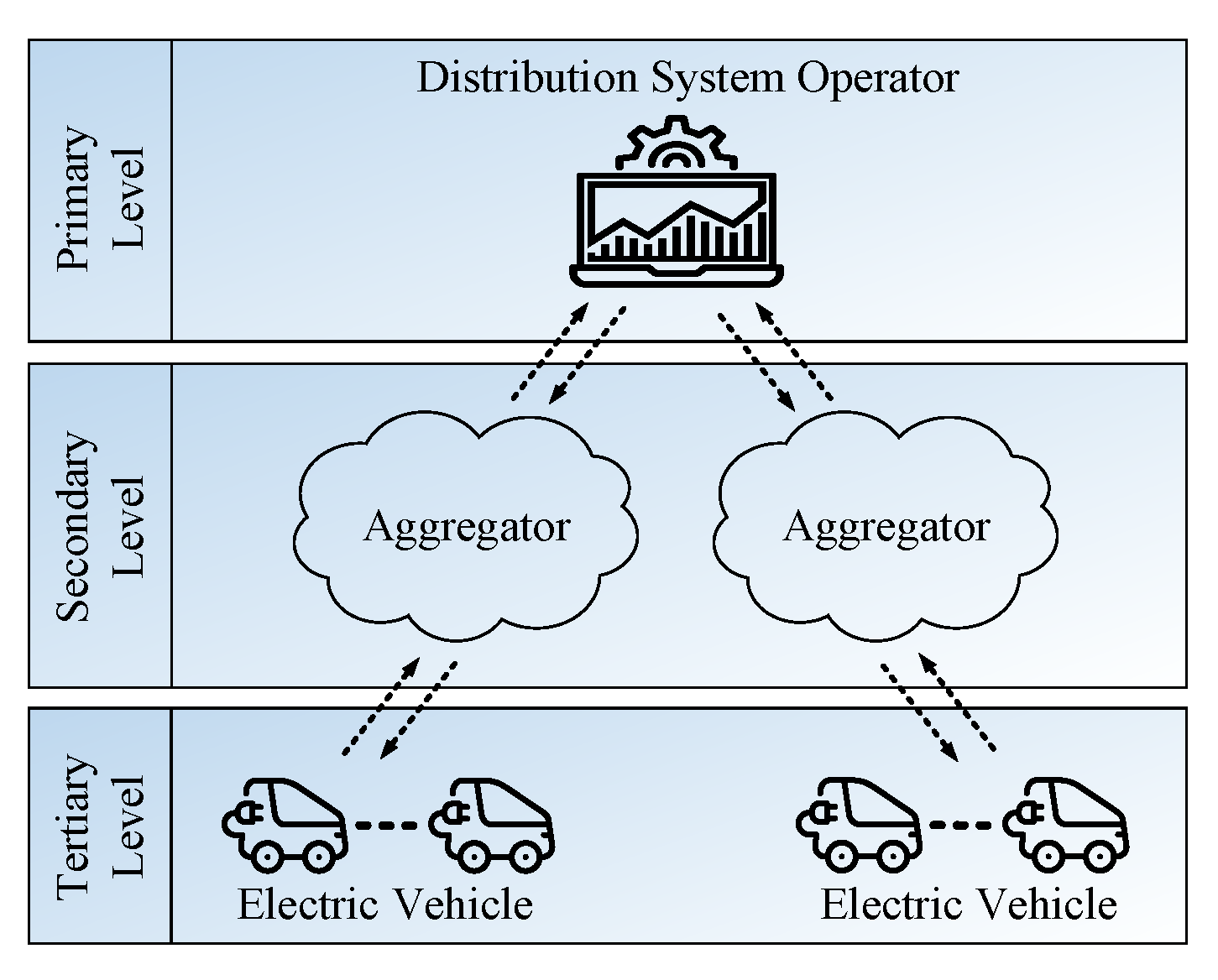
Though EVs can be capitalized for V2G/G2V operation individually, the real potential of these EV services is exercised when EVs form a fleet and act as an aggregated storage [5,6,7]. A fleet of EVs under the command of an operator is collectively termed an aggregator. Aggregators act as intermediaries between the distribution system operator (DSO) and EVs. Hierarchical control of EV ancillary services where multiple aggregators are under the jurisdiction of a DSO is more standardized based upon the economical aspects [8]. To smoothen the load profile of the system using EVs, the coordination among the aggregators has to be supervised by the DSO based upon the energy requirements or potential of each aggregator. Concurrently, the aggregators ensure that the driving needs of the EVs are satisfied if they are engaged in grid support.

Recent research has employed the concept of aggregators to govern the management of EVs. The economic benefits of an EV aggregator are analyzed with V2G grid support while complying with the driving needs of EVs in Reference [9]. A simultaneous EV plug-in scenario with equal parking duration is considered, ignoring the essential driving pattern modeling. In Reference [10], charging power allocation of each EV in a parking lot is determined using linear programming in coordination with RE to maximize the profits of the aggregator. A centralized control of EVs has been implemented in Reference [11] to improve the imbalance caused by wind power variations utilizing V2G/G2V techniques. In both these studies [10,11], consideration is not given to the application of EVs to improve the overall load profile from the grid perspective. In Reference [12], V2G has been explored in the form of a single aggregated battery model on a transmission level. Various cases have been simulated with wind power fluctuations, showing a reduction in power exchange deviations. Since the battery model is an aggregated model based on a single EV type, control of individual EVs is neglected. An EV scheduling procedure is designed to minimize the cost for the DSO and parking lot by finding an equilibrium point between the objectives of both entities, along with the consideration of wind power uncertainty [13]. Reference [14] proposes a V2G mechanism for the mitigation of solar energy impact with voltage support functionality. The system design does not consider a proper EV mobility model, as half of the total EVs are assumed to be plugged-in at all times. All these studies are focused on the interaction of a system operator with the EVs aggregated within a single command unit.

Coordination of multiple aggregators for EV charging has been investigated in Reference [15,16]. In Reference [15], a fast heuristic algorithm determines the charging power for all EVs within each aggregator to minimize the charging costs. Reference [16] proposes an adjustable power charging method, which takes into account the EV owner’s preferences to establish a fair dispatch of power among the EV aggregators. Both these schemes aim for peak load reduction without considering V2G, and thus the load variance is only minimized to a certain level. V2G functionalities of EVs to support frequency deviations are studied at a transmission level while considering multiple aggregators [17]. A simplistic approach is used to distribute power among the aggregators without considering the real-time feedback from the EVs under each aggregator’s domain, which can be problematic in practical scenarios. A coordinated control system for EV aggregators and traditional power plants is proposed to decrease the frequency deviations and output power variations of the power plants [18]. The characteristics such as EV dynamics and its initial state-of-charge (SoC) calculation are not incorporated. In Reference [19], the scheduling of EVs under the management of aggregators to provide reserve capacity for the compensation of RE power deviations is proposed. The results suggest that the peak load demand of the system did not increase, although the mechanism to achieve the objective to flatten the load profile is not discussed. Furthermore, the aspect regarding the unavailability of required EV SoC at the customer’s desired time and the resultant cancellation of the trip is unfeasible. Reference [20] proposes a hierarchical control of EVs to support the RE intermittency, thus minimizing the dependency for backup generation to reduce the system operation cost. Overall, the research lacks a coordination procedure among multiple aggregators to execute V2G/G2V for load profile smoothing together with RE accommodation.

The minimization of load variance and adherence of the load profile to its target value establishes the potential for further load addition without network reinforcement. Numerous studies have considered the application of EVs to achieve this objective. A peak shaving and valley filling technique is proposed in Reference [21] for the achievement of the target load profile with V2G/G2V. The aspects of EV mobility are not considered in this study. Reference [22] showed that a coordinated control algorithm can be implemented to attain almost similar results to the optimal solution as defined by the objective function in Reference [21] with less computational burden. However, employing a higher EV penetration rate results in the rebounding effect with another peak occurring at the off-peak hours during EV charging. A distributed price-based coordination control of EVs is proposed in Reference [23] with the incorporation of RE. The scheme is not applicable for a large-scale occupation of EVs and the load variance abatement operation is based upon forecasting. In addition, real-time scenarios are not considered.

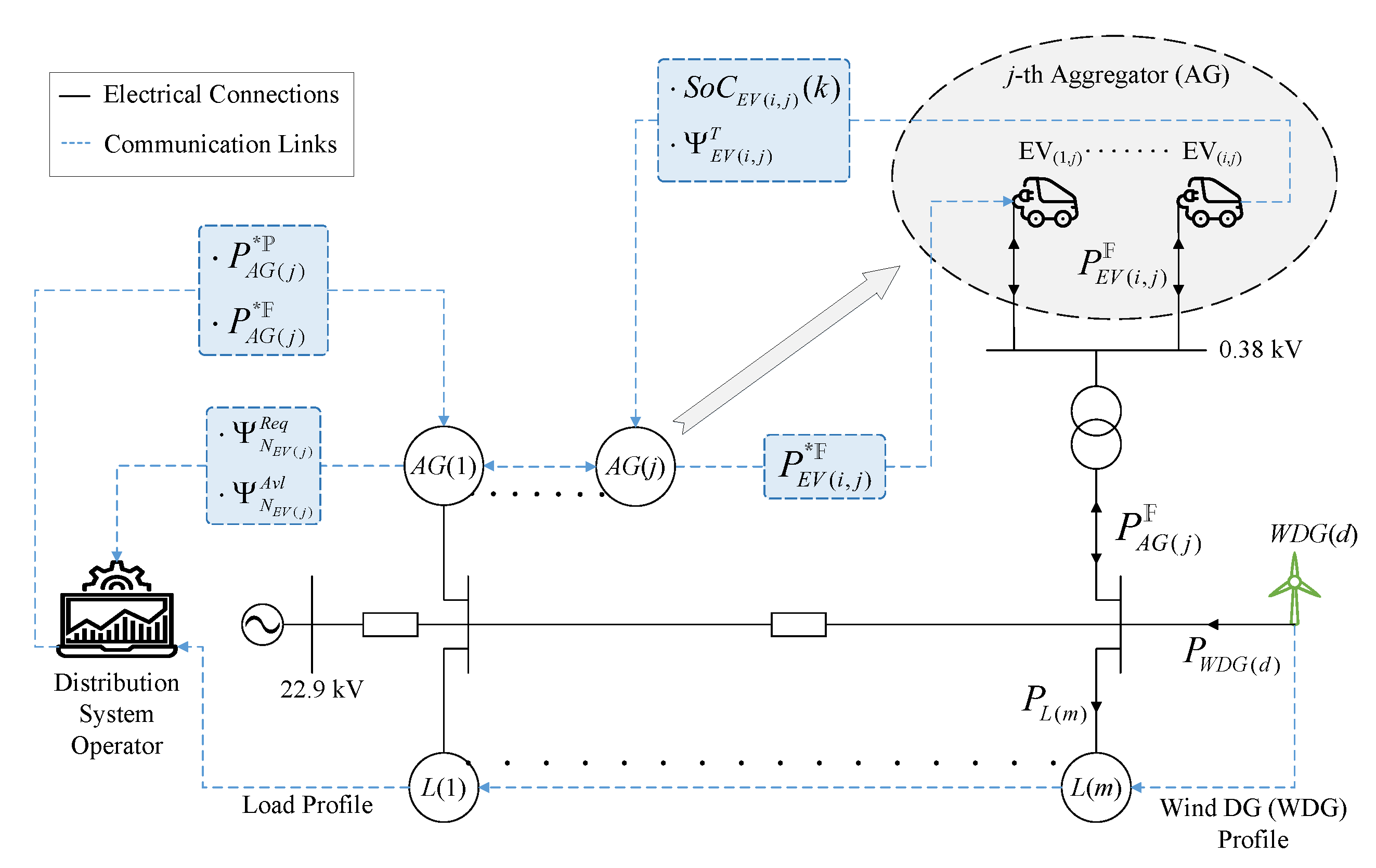
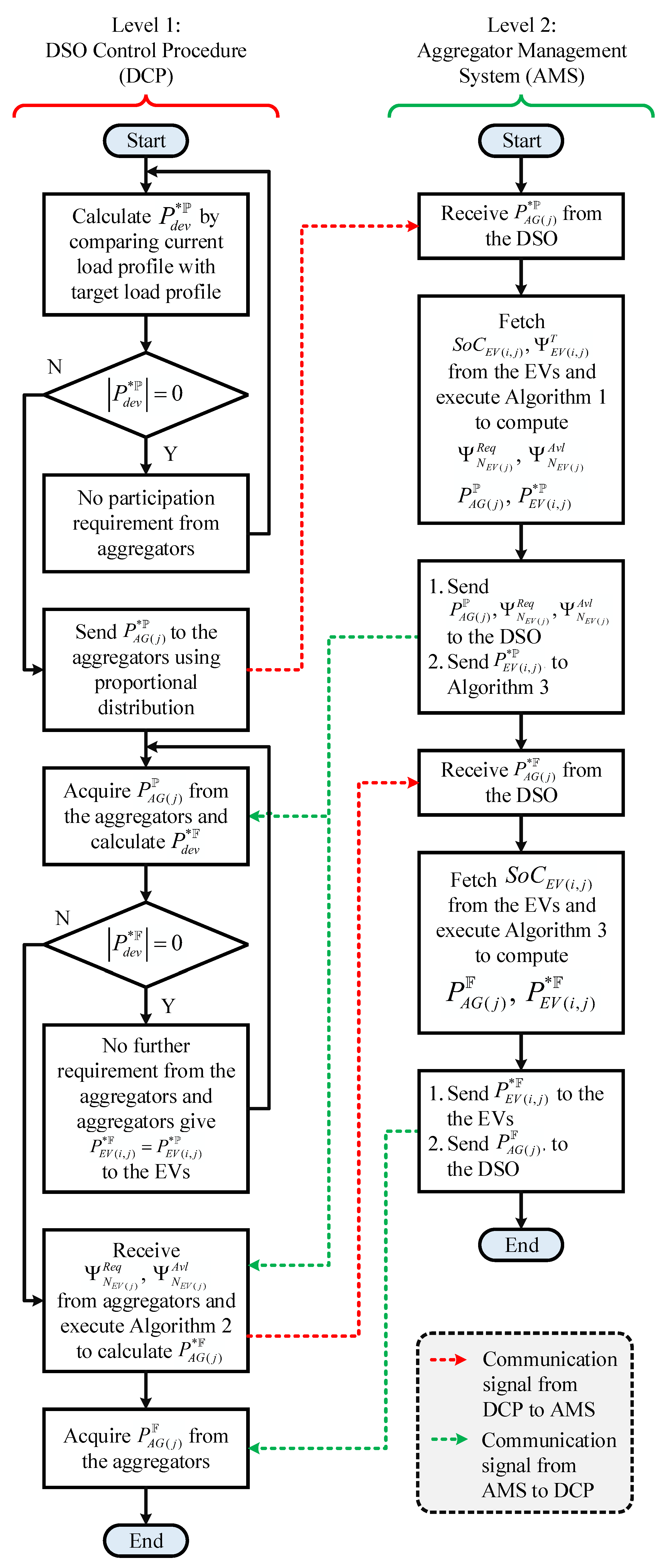
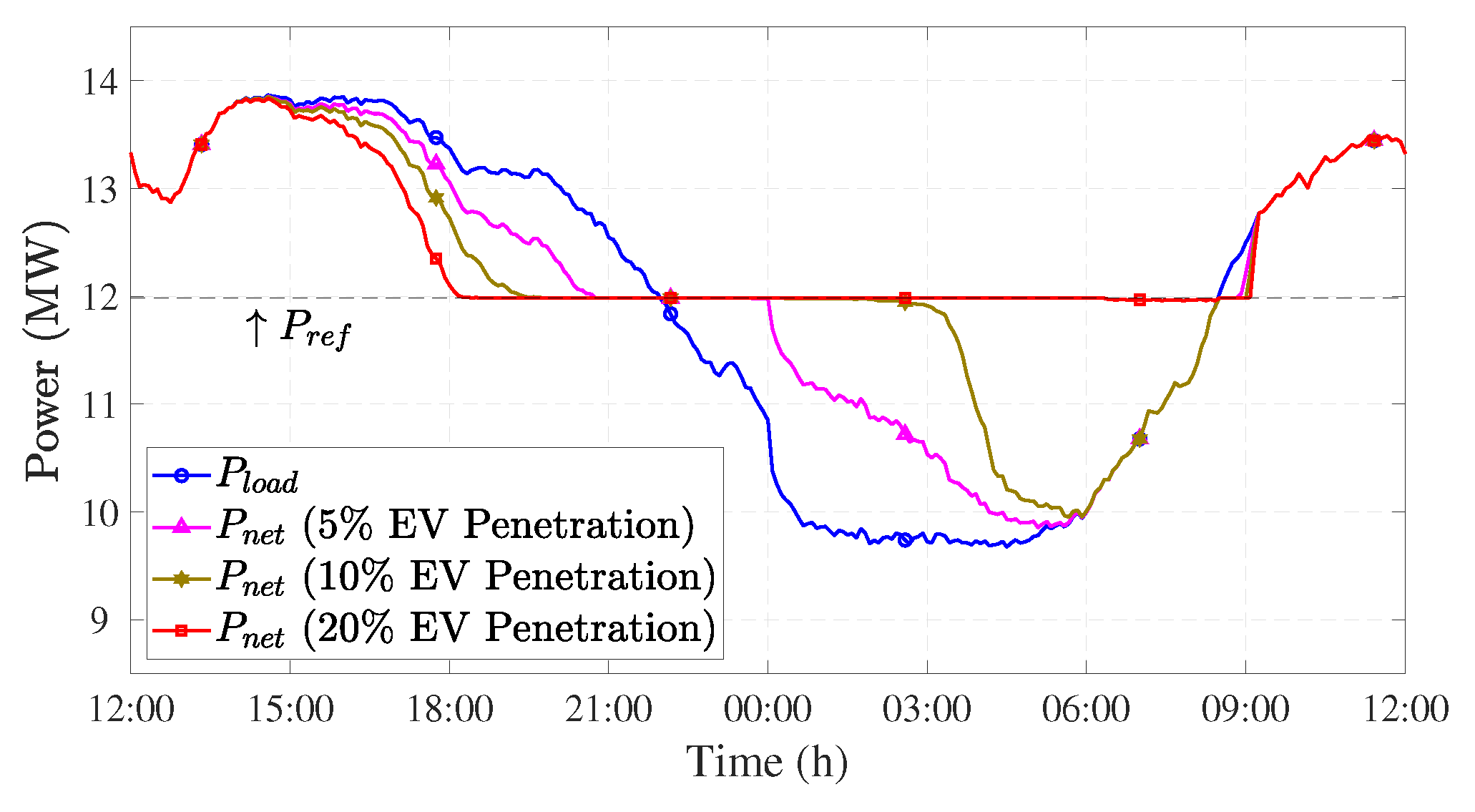
In this paper, we have proposed a multiple aggregator coordination strategy to utilize the EVs for grid support. The design is composed of a bi-level structure: an upper-level system implemented at the DSO, called the DSO control procedure (DCP) which regulates all the aggregators, and a lower level control which is executed at each aggregator to manage the EVs, termed as the aggregator management system (AMS). The scheme employs the V2G/G2V operation to pursue the objectives of peak load reduction and valley filling whilst considering the stochastic mobility characteristics of EVs, and thus fulfills their driving needs. The AMS executes a decisive procedure based upon a water-filling (WF) algorithm to allocate power to the EVs. The competence of the proposed methodology is verified on a real medium voltage (MV) distribution system located in Seoul, Korea. The respective traffic volume data of the feeder regarding its load locations and vehicle mobility trends in Korea are adopted. Various factors are defined to asses the effectiveness of the scheme under different study cases such as comparison with uncontrolled EV charging and different EV penetration levels. The adaptivity of the method to RE incorporation is also tested, where EVs tend to compensate for the RE intermittency and aim for load variance minimization simultaneously. Lastly, the performance of the proposed strategy is compared with an existing load leveling scheme to show its significance.

As such, the proposed scheme is a rigorous methodology which integrates the important aspects of the previous literature such as multiple aggregators coordination, RE compensation, and load curve flattening through EV support, and it utilizes a fast WF method for its operation. The main contributions of this work can be summarized as follows:

• A coordination approach for multiple EV aggregators is proposed to smoothen the system load profile. The hierarchical control structure provides an efficient interaction over all levels using a bi-directional flow and fulfills the objectives at each level.
• The scheme operates in an on-line fashion without the requirement of off-line forecasting, which makes it favorable for RE induction.
• The bi-level algorithm is fast and does not require heavy iterative computations even when the number of EVs is large.
• The proposed method has a better performance than Reference [22] as indicated in the results.

The rest of the paper is organized as follows: Section 2 presents the overall system architecture and states the modeling of the EVs. Section 3 gives a detailed insight into the proposed bi-level coordination scheme in a step-by-step approach. The simulation cases are outlined in Section 4. A thorough illustration and discussion of the results obtained from the study cases are given in Section 5. Section 6 concludes the results and summarizes the findings.

2. System Framework

The propagation of the communication infrastructure is inevitable from the perspective of a smart grid. Its main aim is to enable active interaction among various role-players in the power system: from the top level system operator to the end-user. The process of standardizing the communication channels to transform the conventional grid into a smart grid is already underway [24]. These prospects have paved the way for a transition of centralized infrastructure to a hierarchical form better adapted to the smart grid viewpoint [25].

With the EVs emerging as important service providers in the modern grid, their increasing number will increase the decision variables associated with them. Therefore, accommodating them calls for novel management procedures based upon a hierarchical framework.

The hierarchical control flow model considered in this study consists of three levels: DSO, Aggregators, and EVs, as shown in Figure 1. DSO is the main command unit at the highest level located at the MV substation and it receives the information regarding the power profiles of the loads and the renewable DGs in the feeder. The information exchange between the EVs and the DSO is mediated through an aggregator which is located at the secondary level. The aggregator presents itself to the DSO as a large battery storage unit. The job of the aggregator is to supervise all the EVs under its domain and provide a link to the DSO. Once the aggregator receives the power request signal from the DSO according to the requirements of the grid, it manages the charging or discharging of EVs by giving individual power commands to them constrained to an EV owner’s satisfaction.

2.1. Development of the EV Model

2.1.1. EV Mobility

The information input regarding the EV dynamics is vital to assess the practicality of any grid support strategy. Gaussian distribution can be used to model the mobility parameters such as home arrival time of EVs and the daily distance they travel [15,22].

In this study, the total duration of a day is divided into K number of time slots with $\Delta t$ as the interval length. Each time slot is indexed as $k|k\in \left\{1,2,\dots ,K\right\}$. As such, the arrival times $k_{AT}$ of EVs are determined by using Gaussian random distribution function as follows:

$$f(k_{AT},{\mu }_{AT},{\sigma }_{AT})=\left[\frac{1}{{\sigma }_{AT}\sqrt{2\pi }}{e}^{-\frac{{(k-{\mu }_{AT})}^2}{2{\sigma }_{AT}^2}}\right]\times \frac{1}{\Delta t};k_{AT}>0$$

(1)

Similarly, the daily trip distance $DD$ is calculated from Equation (2):

$$f(DD,{\mu }_{DD},{\sigma }_{DD})=\frac{1}{{\sigma }_{DD}\sqrt{2\pi }}{e}^{-\frac{{(t-{\mu }_{DD})}^2}{2{\sigma }_{DD}^2}};DD>0$$

(2)

Furthermore, Monte Carlo simulations are used to determine the departure time $k_{DT}$ of EVs [26].

2.1.2. EV Architecture

Since we are considering both the charging and discharging of EVs, the EV chargers are assumed to be capable of bidirectional power transfer. The i-th EV updates its SoC to the j-th aggregator upon arrival and being plugged-in. Furthermore, the total battery capacity ${\Psi }_{EV(i,j)}^T$ is also reported to the aggregator. The initial value of the SoC is based on the distance traveled by the EV. It is calculated as:

$$So{C}_{EV(i,j)}^{Arr}=1-\frac{D{D}_{EV(i,j)}}{R_{EV(i,j)}}$$

(3)

where $D{D}_{EV(i,j)}$ is calculated from Equation (2) and $R_{EV(i,j)}$ is the total driving range of an EV and it is adopted from

Table 1. Specifications of private EVs in Korea.

EV Name	Total Battery Capacity ${\mathbf{\Psi }}_{\mathit{E}\mathit{V}}^{\mathit{T}}$	Range ${\mathit{R}}_{\mathit{E}\mathit{V}}$
	(kWh)	(km)
Kia Soul EV	27	145
Renault Samsung SM3 ZE	26.64	135
Chevrolet GM Spark	18.3	128
BMW i3	21.3	132
Nissan Leaf	24.4	132
Hyundai Ioniq	28	191

. It is further established that the EVs should have a specific amount of battery capacity available at all times during their parking duration to be able to cover a minimum distance set for emergency purposes. It also prevents the over-discharging of the EVs. The average driving distance mentioned in

Table 2. Private vehicles mobility data of Korea.

Parameter	Average $\mathit{\mu }$	Standard Deviation $\mathit{\sigma }$
Arrival time [35]	19:00 h	2 h
Driving Distance [36]	38.8 km	21.9 km

is assumed as the minimum distance requirement in this study. Therefore, the minimum battery SoC of each EV is calculated as:

$$So{C}_{EV(i,j)}^{min}=\frac{{\mu }_{DD}}{R_{EV(i,j)}}$$

(4)

so that the battery capacity ${\Psi }_{EV(i,j)}^{Avl(min)}={\Psi }_{EV(i,j)}^T\times So{C}_{EV(i,j)}^{min}$ kWh should be available in each EV for the corresponding minimum distance travel.

Equation (5) indicates the EV power $P_{EV(i,j)}^{\mathbb{F}}\left(k\right)$ at each time slot k:

$$P_{EV(i,j)}^{\mathbb{F}}\left(k\right)=P_{EV(i,j)}^{*\mathbb{F}}\left(k\right)\times {\rho }_{EV(i,j)}{S}_{EV(i,j)}$$

(5)

where the reference power $P_{EV(i,j)}^{*\mathbb{F}}\left(k\right)$ is received from the aggregator. The factor ${\rho }_{EV(i,j)}$ is the plug-in status of the EV where 1 = plugged-in and 0 = unplugged:

$${\rho }_{EV(i,j)}=\left\{\begin{array}{cc}1\hfill & \forall k\in \left[k_{EV(i,j)}^{AT},k_{EV(i,j)}^{DT}\right]\hfill \\ 0\hfill & \mathrm{otherwise}\hfill \end{array}\right.$$

(6)

The term $S_{EV(i,j)}$ is the SoC state signal and it is defined as below:

$$S_{EV(i,j)}=\left\{\begin{array}{cc}1\hfill & P_{EV(i,j)}^{*\mathbb{F}}>0\wedge So{C}_{EV(i,j)}\le So{C}_{EV(i,j)}^{Dep}|P_{EV(i,j)}^{*\mathbb{F}}<0\wedge So{C}_{EV(i,j)}\ge So{C}_{EV(i,j)}^{min}\hfill \\ 0\hfill & \mathrm{otherwise}\hfill \end{array}\right.$$

(7)

where $So{C}_{EV(i,j)}^{Dep}\le So{C}_{EV(i,j)}^{max}$, the maximum value of SoC being 100%. At each time interval k, the value of the current SoC is updated to the aggregator:

$$So{C}_{EV(i,j)}\left(k\right)=So{C}_{EV(i,j)}(k-1)+\frac{P_{EV(i,j)}^{\mathbb{F}}\left(k\right)}{{\Psi }_{EV(i,j)}^T}\frac{\Delta t}{60}$$

(8)

Since the EV is considered as a load source, a positive power indicates charging and negative power implies discharging of the EV battery.

Figure 2 shows the overall system framework. The two-way communication is established among the DSO, aggregators, and EVs. Information flow from the loads and DGs to the DSO is one-way as these entities are autonomous.

3. Bi-Level Coordination Scheme

In this study, a coordination scheme is developed to smoothen the load profile by utilizing the EVs. The main control structure is bi-level which is implemented at the DSO and the aggregators, although two-way information flow from the tertiary level EVs is also practiced. The first level control DCP is administered at the substation level directed by the DSO and its subsidiaries are the aggregators. The second level control AMS is implemented at each aggregator and its job is to coordinate all the EVs under its authority. The objectives of the two levels can be summarized as:

• The main purpose of the DCP is to flatten the net load curve by reducing the peak load, filling the valley period and thus decreasing the overall load variance. As such, it tends to reduce the difference between the target load profile and the net load profile incorporating EVs. This prospect can be represented by the following objective:

  $$\left\{\begin{array}{c}min\left[P_{ref}-\left(P_{load}+{\displaystyle \sum _{j=1}^{N_{AG}}\sum _{i=1}^{N_{EV\left(j\right)}}}{P}_{EV(i,j)}^{\mathbb{F}}\right)\right]\hfill \\ \mathrm{s}.\mathrm{t}.\hfill \\ 0\le \left|P_{EV(i,j)}^{\mathbb{F}}\right|\le \left|P_{EV}^{RTD}\right|,\forall i\in \left\{1,\dots ,N_{EV\left(j\right)}\right\},\forall j\in \left\{1,\dots ,N_{AG}\right\}\hfill \\ \sum _{j=1}^{N_{AG}}\sum _{i=1}^{N_{EV\left(j\right)}}{P}_{EV(i,j)}^{\mathbb{F}}\le P_{dev}^{*\mathbb{P}}\hfill \end{array}\right.$$

  (9)

  where $P_{ref}$ is the target load profile, ideally a flat curve, and in this study, it is based on the average value of the daily load profile as set by the DSO, $P_{load}$ is calculated by accumulating the loads on all the feeder buses as given by Equation (10), and $P_{dev}^{*\mathbb{P}}$ is the provisional value of the power deviation from the target load profile as calculated in Equation (11). The secondary objective of DCP is the coordination among the aggregators keeping in view their energy requirements.

  $$P_{load}=\sum _{m=1}^{N_L}{P}_{L\left(m\right)}$$

  (10)

• The objective of the AMS is to fulfill the driving requirements of EVs, in addition to fulfilling its duty as a subsidiary to the DCP. The EVs are charged/discharged while maintaining their minimum driving needs and they are provided with a full SoC before departure.

3.1. Scheme Description

The detailed control flow process of the coordination scheme executed at each time slot is displayed in Figure 3. The figure shows the simultaneous operation of both levels of the scheme and the two-way communication between them. The scheme is composed of three sub-algorithms. The scheme is adaptive to the incoming and outgoing EVs, and the status of all EVs is updated at each time interval. A step-by-step illustration of various stages of the scheme is mentioned ahead.

3.1.1. Step 1: Calculation of Provisional Power Mismatch

Assume that the number of aggregators is $N_{AG}$, where $j\in \left\{1,2,\dots ,N_{AG\left(j\right)}\right\}$ is the index of aggregators. The projection of feeder load at each time slot k and the corresponding power output of the j-the aggregator is depicted by the three-dimensional power allocation model, as illustrated in the $k-j$ plane in Figure 4. The DCP calculates the provisional power deviation $P_{dev}^{*\mathbb{P}}$ from the target load profile $P_{ref}$ set by the DSO as given in Equation (11):

$$P_{dev}^{*\mathbb{P}}=P_{ref}-P_{load}$$

(11)

On the basis of this mismatch, the provisional power allocation to aggregators $P_{AG\left(j\right)}^{*\mathbb{P}}$ is carried out by the DCP based on a fair proportional division:

$$P_{AG\left(j\right)}^{*\mathbb{P}}=\frac{N_{EV\left(j\right)}}{{\sum }_{j=1}^{N_{AG}}{N}_{EV\left(j\right)}}{P}_{dev}^{*\mathbb{P}}$$

(12)

During each time slot k, the aggregators tend to match their energy requirements based on the availability of EVs within their domain. If $P_{load}>P_{ref}$ then $P_{dev}^{*\mathbb{P}}$ is negative, which corresponds to V2G operation. If $P_{load}<P_{ref}$ then $P_{dev}^{*\mathbb{P}}$ is positive, and the EVs are charged.

3.1.2. Step 2: Provisional EV Power Allocation

In this step, the AMS executes Algorithm 1 at each aggregator to obtain the provisional power reference $P_{EV(i,j)}^{*\mathbb{P}}$ for all the EVs under its supervision. Firstly, the aggregator collects data from the EVs such as their battery SoC and rated capacity, which is used to calculate each EV’s available battery capacity ${\Psi }_{EV(i,j)}^{Avl}$ and required battery capacity for full charge ${\Psi }_{EV(i,j)}^{Req}$ given by:

$${\Psi }_{EV(i,j)}^{Avl}={\Psi }_{EV(i,j)}^T\times So{C}_{EV(i,j)}$$

(13)

$${\Psi }_{EV(i,j)}^{Req}={\Psi }_{EV(i,j)}^T-{\Psi }_{EV(i,j)}^{Avl}$$

(14)

On the basis of the power allotted to aggregator $P_{AG\left(j\right)}^{*\mathbb{P}}$, a provisional power reference is calculated for each EV according to its battery capacity requirement or potential. Afterwards, the AMS at each aggregator computes the total provisional power $P_{AG\left(j\right)}^{\mathbb{P}}$ from all EVs under its domain as defined by Equation (15):

$$P_{AG\left(j\right)}^{\mathbb{P}}=\sum _{i=1}^{N_{EV\left(j\right)}}{P}_{EV(i,j)}^{*\mathbb{P}}$$

(15)

Algorithm 1 Provisional EV Power Allocation

Input:$P_{AG\left(j\right)}^{*\mathbb{P}}$, $P_{EV}^{RTD}$, ${SoC}_{EV(i,j)}$, ${\Psi }_{EV(i,j)}^T$, $i=1,\dots ,N_{EV\left(j\right)}$, $j=1,\dots ,N_{AG}$

Output:$P_{AG\left(j\right)}^{\mathbb{P}}$, $P_{EV(i,j)}^{*\mathbb{P}}$, ${\Psi }_{N_{EV\left(j\right)}}^{Req}$, ${\Psi }_{N_{EV\left(j\right)}}^{Avl}$, $i=1,\dots ,N_{EV\left(j\right)}$, $j=1,\dots ,N_{AG}$   1: Each $E{V}_{(i,j)}$, $i=1,\dots ,N_{EV\left(j\right)}$ of j-th aggregator reports its $So{C}_{EV(i,j)}$ and ${\Psi }_{EV(i,j)}^T$ to the control   2: Calculate ${\Psi }_{N_{EV\left(j\right)}}^{Avl}$ and ${\Psi }_{N_{EV\left(j\right)}}^{Req}$▹ total available battery capacity and total required battery capacity of all EVs of j-th aggregator, respectively ↳ ${\Psi }_{N_{EV\left(j\right)}}^{Avl}={\sum }_{i=1}^{N_{EV\left(j\right)}}\left({\Psi }_{EV(i,j)}^T\times So{C}_{EV(i,j)}\right)$ ↳ ${\Psi }_{N_{EV\left(j\right)}}^{Req}={\sum }_{i=1}^{N_{EV\left(j\right)}}\left({\Psi }_{EV(i,j)}^T-{\Psi }_{EV(i,j)}^{Avl}\right)$   3: if$P_{AG\left(j\right)}^{*\mathbb{P}}>0$then   4:     for $i=1,\dots ,N_{EV\left(j\right)}$ do   5:         $P_{EV(i,j)}^{*\mathbb{P}}=\left({\Psi }_{EV(i,j)}^{Req}/{\Psi }_{N_{EV\left(j\right)}}^{Req}\right)\times P_{AG\left(j\right)}^{*\mathbb{P}}$   6:         if $P_{EV(i,j)}^{*\mathbb{P}}>P_{EV}^{RTD}$ then   7:            $P_{EV(i,j)}^{*\mathbb{P}}=P_{EV}^{RTD}$   8:         end if   9:         if ${\Psi }_{N_{EV\left(j\right)}}^{Req}=0$ then 10:            $P_{EV(i,j)}^{*\mathbb{P}}=0$ 11:         end if 12:     end for 13: else if$P_{AG\left(j\right)}^{*\mathbb{P}}<0$then 14:     for $i=1,\dots ,N_{EV\left(j\right)}$ do 15:         $P_{EV(i,j)}^{*\mathbb{P}}=\left({\Psi }_{EV(i,j)}^{Avl}/{\Psi }_{N_{EV\left(j\right)}}^{Avl}\right)\times P_{AG\left(j\right)}^{*\mathbb{P}}$ 16:         if $P_{EV(i,j)}^{*\mathbb{P}}<-P_{EV}^{RTD}$ then 17:            $P_{EV(i,j)}^{*\mathbb{P}}=-P_{EV}^{RTD}$ 18:         end if 19:         if ${\Psi }_{N_{EV\left(j\right)}}^{Avl}=0$ then 20:            $P_{EV(i,j)}^{*\mathbb{P}}=0$ 21:         end if 22:     end for 23: else 24:     for $i=1,\dots ,N_{EV\left(j\right)}$ do 25:         $P_{EV(i,j)}^{*\mathbb{P}}=0$ 26:     end for 27: end if 28: Compute Equation (15) to obtain $P_{AG\left(j\right)}^{\mathbb{P}}$

3.1.3. Step 3: Calculation of Final Power Mismatch and Aggregator Coordination

The term $P_{AG\left(j\right)}^{\mathbb{P}}$ determined by the AMS is sent to the DCP to calculate the final power deviation $P_{dev}^{*\mathbb{F}}$ from target load profile whilst also incorporating the provisional powers of the EVs (Equation (16)).

$$P_{dev}^{*\mathbb{F}}=P_{ref}-\left(P_{load}+\sum _{j=1}^{N_{AG}}{P}_{AG\left(j\right)}^{\mathbb{P}}\right)$$

(16)

The DCP also receives the required and available aggregated battery capacity of all EVs within each aggregator’s domain. Subsequently, it executes Algorithm 2 to coordinate the final power allocation reference $P_{AG\left(j\right)}^{*\mathbb{F}}$ dispatch among the aggregators based upon their respective demand or capability.

Algorithm 2 Aggregator Coordination

Input:$P_{dev}^{*\mathbb{F}}$, ${\Psi }_{N_{EV\left(j\right)}}^{Req}$, ${\Psi }_{N_{EV\left(j\right)}}^{Avl}$, $j=1,\dots ,N_{AG}$

Output:$P_{AG\left(j\right)}^{*\mathbb{F}}$, $j=1,\dots ,N_{AG}$   1: for$j=1,\dots ,N_{AG}$do   2:     ${\gamma }_{\left(j\right)}={\Psi }_{N_{EV\left(j\right)}}^{Req}/N_{EV\left(j\right)}$   ▹${\gamma }_{\left(j\right)}$ is the required battery capacity factor of j-th aggregator   3:     ${\alpha }_{\left(j\right)}={\Psi }_{N_{EV\left(j\right)}}^{Avl}/N_{EV\left(j\right)}$   ▹${\alpha }_{\left(j\right)}$ is the available battery capacity factor of j-th aggregator   4: end for   5: Compute ${\sum }_{j=1}^{N_{AG}}{\gamma }_{\left(j\right)}$, $j=1,\dots ,N_{AG}$   6: Compute ${\sum }_{j=1}^{N_{AG}}{\alpha }_{\left(j\right)}$, $j=1,\dots ,N_{AG}$   7: if$P_{dev}^{*\mathbb{F}}>0$then   8:     for $j=1,\dots ,N_{AG}$ do   9:         $P_{AG\left(j\right)}^{*\mathbb{F}}=\left({\gamma }_{\left(j\right)}/{\sum }_{j=1}^{N_{AG}}{\gamma }_{\left(j\right)}\right)\times P_{dev}^{*\mathbb{F}}$ 10:         if ${\sum }_{j=1}^{N_{AG}}{\gamma }_{\left(j\right)}=0$ then 11:            $P_{AG\left(j\right)}^{*\mathbb{F}}=0$ 12:         end if 13:     end for 14: else if$P_{dev}^{*\mathbb{F}}<0$then 15:     for $j=1,\dots ,N_{AG}$ do 16:         $P_{AG\left(j\right)}^{*\mathbb{F}}=\left({\alpha }_{\left(j\right)}/{\sum }_{j=1}^{N_{AG}}{\alpha }_{\left(j\right)}\right)\times P_{dev}^{*\mathbb{F}}$ 17:         if ${\sum }_{j=1}^{N_{AG}}{\alpha }_{\left(j\right)}=0$ then 18:            $P_{AG\left(j\right)}^{*\mathbb{F}}=0$ 19:         end if 20:     end for 21: else 22:     for $j=1,\dots ,N_{AG}$ do 23:         $P_{AG\left(j\right)}^{*\mathbb{F}}=0$ 24:     end for 25: end if

3.1.4. Step 4: Water-Filling Algorithm and Final EV Power Allocation

Once the aggregators receive their final power allocation reference, each AMS executes Algorithm 3 based on a water-filling (WF) algorithm to compute the final power reference for the EVs. The WF algorithm has been widely used for power allotment in communication systems. It has recently found its application in power systems for load management techniques as employed by Reference [27,28].

The AMS has to divide the power $P_{AG\left(j\right)}^{*\mathbb{F}}$ among all the EVs within the aggregator. On the basis of the water-filling algorithm principles, the EVs are sorted in accordance with their current SoC level. EVs are arranged in monotonically increasing order of their SoC values for a charging scenario and therefore, those EVs with lowest SoC value are allocated supplemental charging power reference $P_{EV(i,j)}^{\varpi }$ earlier (Figure 5a). As for the discharging action of EVs, they are arranged in monotonically decreasing order of their SoC values and higher SoC EVs are allotted supplemental discharging power reference $P_{EV(i,j)}^{\varpi }$ beforehand (Figure 5b). $P_{AG\left(j\right)}^{*\mathbb{F}}$ is depicted by the water level above the i-th EV in Figure 5. The water level steps down once the shaded portion $P_{EV(i,j)}^{\varpi }$ is extracted from it.

Finally, the EV power calculated from the WF algorithm $P_{EV(i,j)}^{\varpi }$ is appended to the provisional power reference to obtain the final power allocation reference $P_{EV(i,j)}^{*\mathbb{F}}$ for the EVs as shown in Figure 6. The charging or discharging power of the EV is constrained by the rated charger capacity $P_{EV}^{RTD}$.

Algorithm 3 Water Filling Algorithm for EVs

Input:$P_{AG\left(j\right)}^{*\mathbb{F}}$, $P_{EV}^{RTD}$, $P_{EV(i,j)}^{*\mathbb{P}}$, ${SoC}_{EV(i,j)}$, $j=1,\dots ,N_{EV\left(j\right)}$, $j=1,\dots ,N_{AG}$

Output:$P_{AG\left(j\right)}^{\mathbb{F}}$, $P_{EV(i,j)}^{*\mathbb{F}}$, $i=1,\dots ,N_{EV\left(j\right)}$, $j=1,\dots ,N_{AG}$   1: Sort j-th aggregator EVs in ascending order of their SoC ↳ $\forall i,sor{t}_{\uparrow }\left\{So{C}_{EV(i,j)}\right\}\to \left\{So{C}_{EV(i_{\uparrow },j)}\right\},i_{\uparrow }=1,\dots ,N_{EV\left(j\right)}$  ▹$i_{\uparrow }$ is the index of EVs in ascending order of their SoC   2: Sort j-th aggregator EVs in descending order of their SoC ↳ $\forall i,sor{t}_{\downarrow }\left\{So{C}_{EV(i,j)}\right\}\to \left\{So{C}_{EV(i_{\downarrow },j)}\right\},i_{\downarrow }=1,\dots ,N_{EV\left(j\right)}$  ▹$i_{\downarrow }$ is the index of EVs in descending order of their SoC   3: if$P_{AG\left(j\right)}^{*\mathbb{F}}>0$then   4:     for $i_{\uparrow }=1,\dots ,N_{EV\left(j\right)}$ do   5:         if $P_{EV(i_{\uparrow },j)}^{*\mathbb{P}}=P_{EV}^{RTD}|P_{EV(i_{\uparrow },j)}^{*\mathbb{P}}=0$ then   6:            $P_{EV(i_{\uparrow },j)}^{\varpi }=0$   7:         else   8:            $P_{EV(i_{\uparrow },j)}^{\varpi }=P_{EV}^{RTD}-P_{EV(i_{\uparrow },j)}^{*\mathbb{P}}$   9:            if $P_{EV(i_{\uparrow },j)}^{\varpi }>P_{AG\left(j\right)}^{*\mathbb{F}}$ then 10:                $P_{EV(i_{\uparrow },j)}^{\varpi }=0$ 11:            end if 12:            $P_{AG\left(j\right)}^{*\mathbb{F}}=P_{AG\left(j\right)}^{*\mathbb{F}}-P_{EV(i_{\uparrow },j)}^{\varpi }$ 13:         end if 14:     end for 15: else if$P_{AG\left(j\right)}^{*\mathbb{F}}<0$then 16:     for $i_{\downarrow }=1,\dots ,N_{EV\left(j\right)}$ do 17:         if $P_{EV(i_{\downarrow },j)}^{*\mathbb{P}}=-P_{EV}^{RTD}|P_{EV(i_{\downarrow },j)}^{*\mathbb{P}}=0$ then 18:            $P_{EV(i_{\downarrow },j)}^{\varpi }=0$ 19:         else 20:            $P_{EV(i_{\downarrow },j)}^{\varpi }=-P_{EV}^{RTD}-P_{EV(i_{\downarrow },j)}^{*\mathbb{P}}$ 21:            if $P_{EV(i_{\downarrow },j)}^{\varpi }<P_{AG\left(j\right)}^{*\mathbb{F}}$ then 22:                $P_{EV(i_{\downarrow },j)}^{\varpi }=0$ 23:            end if 24:            $P_{AG\left(j\right)}^{*\mathbb{F}}=P_{AG\left(j\right)}^{*\mathbb{F}}-P_{EV(i_{\downarrow },j)}^{\varpi }$ 25:         end if 26:     end for 27: else 28:     for $i=1,\dots ,N_{EV\left(j\right)}$ do 29:         $P_{EV(i,j)}^{\varpi }=0$ 30:     end for 31: end if 32: for$i=1,\dots ,N_{EV\left(j\right)}$do 33:     $P_{EV(i,j)}^{*\mathbb{F}}=P_{EV(i,j)}^{*\mathbb{P}}+P_{EV(i,j)}^{\varpi }$ 34: end for 35: Fetch $P_{EV(i,j)}^{\mathbb{F}}$ from Equation (5) and compute ${\sum }_{i=1}^{N_{EV\left(j\right)}}{P}_{EV(i,j)}^{\mathbb{F}}$ to obtain $P_{AG\left(j\right)}^{\mathbb{F}}$

3.1.5. Step 5: Net Power Transfer from the Grid

Once all the EVs receive their power allocation reference, they execute their charging or discharging process depending upon the reference power. Finally, the net power transfer from the grid $P_{net}$ can be calculated from Equation (17):

$$P_{net}=P_{load}+\sum _{j=1}^{N_{AG}}{P}_{AG\left(j\right)}^{\mathbb{F}}$$

(17)

This is the load profile which has been flattened by the bi-level coordination scheme and it includes the total EV load. The total energy provided or consumed by the EVs may be lower than the total requirement $P_{dev}^{*\mathbb{P}}$ calculated initially, therefore the remaining amount is acquired from the grid.

4. Simulation Cases

4.1. MV Distribution Feeder

The proposed scheme has been tested on a distribution feeder located in Seoul, Korea. The accurate traffic volume is available for the southern part of the feeder. Therefore, the simulation cases are carried out on the southern feeder with relevant EV statistics. The southern feeder, named X S/S - Z D/L, has a total length of 9.331 km and the total load is 13.866 MW divided among 11 locations from L1 to L11 [29]. The single-line diagram of the feeder is illustrated in Figure 7.

The daily load profile of the feeder follows the daily demand pattern of Korea. The maximum and minimum range of load capacity is highest in the summer season among the four seasons, hence we consider the summer load profile for the simulation cases as the worst case scenario [30]. The feeder load profile for a summer day is shown in Figure 8. The 13.9 MW peak demand occurs around 14:30 whereas the lowest load value of 9.7 MW occurs at about 04:30. The target load profile is a flat curve represented by $P_{ref}$ in the Figure 8 and its value is approximately 12 MW.

4.2. EV Fleet

According to Reference [31], the number of EVs in the vicinity of each load location of the feeder has been established. All the EVs within a specific load location are under the domain of the respective aggregator. The total number of vehicles in the feeder locality is 8961. Accordingly, the 5%, 10%, and 20% EV penetration levels considered in the simulation cases are presented in

Table 3. Electric vehicle (EV) penetration levels in the feeder.

Location	Aggregator	Number of EVs
		5% Penetration	10% Penetration	20% Penetration
L1	AG1	38	77	154
L2	AG2	13	25	50
L3	AG3	27	54	108
L4	AG4	58	116	232
L5	AG5	18	36	72
L6	AG6	23	47	94
L7	AG7	39	77	154
L8	AG8	38	77	154
L9	AG9	42	83	166
L10	AG10	10	20	40
L11	AG11	142	284	568
Total		448	896	1792

.

The EV fleet consists of various EVs commonly available in Korea. The specifications of the EVs considered in this study, such as their rated battery capacity and total driving range, are acquired from Reference [32] and given in Table 1. Currently, about 95% of EV charging is performed using the level-1 chargers generally equipped in residential regions [33]. In Korea, mainly two ratings of personal chargers are available. The 3 kW chargers are commonly used, although 7 kW chargers have also been introduced [34]. The scheme is verified for both charger ratings.

The arrival of EVs in the evening and their subsequent morning departure are in accordance with a residential mobility pattern. The values of the arrival time of EVs and daily driving distance take into consideration the data from the Table 2 regarding home arrival time and driving distance of private vehicles in Korea.

The total time period for each simulation is 24 h. The length of a time slot k is $\Delta t=5$ mins which is in accordance with the data resolutions. As a result, there are a total $K=288$ time slots in a daily 24 h period or 12 time slots per hour. The simulations are executed using the MATLAB 9.3/Simulink 9.0 software environment on a desktop computer with Intel Core i5-3570 CPU @ 3.40GHz/8.00GB RAM/x64-based architecture. The following scenarios are considered to thoroughly verify the performance of the proposed method:

• Uncontrolled charging and proposed methodology comparison: 3 kW and 7 kW charger ratings
• Consideration of various EV penetration levels: 5%, 10%, and 20%
• Proposed scheme adaptability to renewable energy incorporation: 10% and 20% wind power penetration
• Comparison of proposed scheme with a reference scheme

Various entities have been defined to evaluate the effectiveness of the scheme. The power utilization efficiency is given by load factor (LF):

$$\mathrm{LF}(\%)=\frac{\overline{P_{net}}}{P_{net}^{max}}\times 100$$

(18)

where $\overline{P_{net}}$ is given by:

$$\overline{P_{net}}=\frac{1}{K}\sum _{k=1}^K{P}_{net}\left(k\right)$$

(19)

The peak shaving performance is denoted by peak shaving index (PSI) which is the ratio of the total energy shaved by the EVs to the total energy expected to be shaved:

$$\mathrm{PSI}(\%)=\frac{{\sum }_{j=1}^{N_{AG}}{\sum }_{i=1}^{N_{EV\left(j\right)}}{\int }_{k_{peak\left(s\right)}}^{k_{peak\left(e\right)}}{P}_{EV(i,j)}^{\mathbb{F}}\left(k\right)dk}{{\int }_{k_{peak\left(s\right)}}^{k_{peak\left(e\right)}}{P}_{dev}^{*\mathbb{P}}\left(k\right)dk}\times 100$$

(20)

Similarly, the valley filling index (VFI) gives the performance of the scheme due to off-peak EV charging to fill the valley in the load profile:

$$\mathrm{VFI}(\%)=\frac{{\sum }_{j=1}^{N_{AG}}{\sum }_{i=1}^{N_{EV\left(j\right)}}{\int }_{k_{valley\left(s\right)}}^{k_{valley\left(e\right)}}{P}_{EV(i,j)}^{\mathbb{F}}\left(k\right)dk}{{\int }_{k_{valley\left(s\right)}}^{k_{valley\left(e\right)}}{P}_{dev}^{*\mathbb{P}}\left(k\right)dk}\times 100$$

(21)

Finally, the load variance (LV) gives the deviation of the load profile from its average value calculated as follows:

$$\mathrm{LV}=\frac{1}{K}\sum _{k=1}^K{\left|P_{net}\left(k\right)-\overline{P_{net}}\right|}^2$$

(22)

5. Results and Discussion

5.1. Uncontrolled Charging and Proposed Methodology Comparison

In this section, the effectiveness of the proposed scheme is assessed by comparing the results with a free-charging policy of EVs, where the EVs are immediately plugged-in and charged upon arrival . The charging power in such a scenario is given by:

$$P_{EV(i,j)}^{\mathbb{F}}=\left\{\begin{array}{cc}{P}_{EV}^{RTD}\hfill & So{C}_{EV(i,j)}<100\%\hfill \\ 0\hfill & So{C}_{EV(i,j)}=100\%\hfill \end{array}\right.$$

(23)

In the comparison context, two ratings of chargers are considered i.e., 3 kW and 7 kW. The EV penetration level is 10%. Figure 9a,b show the net load profile of the feeder with uncoordinated charging and the proposed method for both charger ratings. The load profile without EVs is also shown for reference. The free-charging method causes the peak load to increase further. For instance, the peak demand rises to 2.3 MW around 19:00 when the highest number of EVs are plugged-in (Figure 9b).

Utilizing our proposed scheme, the EVs are managed to discharge during the peak period to shave the peak and charging is postponed till the off-peak period to fill the valley. The peak load reduction during the top peak hours is limited, as the number of EVs available for V2G around this time is not enough to provide the required power. Once the number of plugged-in EVs is sufficient, the load profile becomes flat and it adheres to the target curve till the early morning hours when the EVs reach their required SoC values. Because of the higher power rating of 7 kW chargers, the duration of the smoothed load profile is longer as depicted in Figure 9.

It has been assumed that all the EVs have set 100% SoC as their expected SoC before the departure. The departing SoC of all EVs are measured and a mean SoC value of 99.07% for 3 kW case and 99.15% for 7 kW case is found, which is an acceptable result for EV owners.

Table 4. Comparison results of various scenarios.

Scenario	Load Factor (LF) (%)	Load Variance (LV) (MW${}^2$)
Without EVs	86.41	2.37
Uncontrolled charging (3 kW chargers)	86.67	2.69
Proposed scheme (3 kW chargers)	88.28	1.15
Uncontrolled charging (7 kW chargers)	85.6	2.87
Proposed scheme (7 kW chargers)	88.4	1.05

gives the comparison results regarding the performance measuring indexes. As a result of the uncoordinated charging of the EVs, the load variance increases further. By applying the proposed method, the load variance is reduced by 57.2% and 63.4% for 3 kW and 7 kW charger cases, respectively. The load factor is also improved.

Aggregator Coordination

This section discusses the results to verify the aggregator coordination circumstances. As discussed earlier, the proposed algorithm initially allocates provisional power references to the aggregators proportionally based upon the number of EVs. Once the feedback from EVs is taken into account by the aggregators regarding their SoC and battery capacities, the final power references are allotted accordingly. This two-step power allocation improves the coordination among the aggregators. To show this improvement, firstly we establish an aggregator contribution factor (ACF) for both V2G and G2V action. The ACF is represented by $\Omega$ and it is defined as:

$${\Omega }_{AG\left(j\right)}^{V2G}=\frac{{\int }_{k_{peak\left(s\right)}}^{k_{peak\left(e\right)}}{P}_{AG\left(j\right)}\left(k\right)dk}{{\sum }_{j=1}^{N_{AG}}{\int }_{k_{peak\left(s\right)}}^{k_{peak\left(e\right)}}{P}_{AG\left(j\right)}\left(k\right)dk}\times 100$$

(24)

$${\Omega }_{AG\left(j\right)}^{G2V}=\frac{{\int }_{k_{valley\left(s\right)}}^{k_{valley\left(e\right)}}{P}_{AG\left(j\right)}\left(k\right)dk}{{\sum }_{j=1}^{N_{AG}}{\int }_{k_{valley\left(s\right)}}^{k_{valley\left(e\right)}}{P}_{AG\left(j\right)}\left(k\right)dk}\times 100$$

(25)

The term $\Delta \Omega ={\Omega }^{\mathbb{F}}-{\Omega }^{\mathbb{P}}$ gives the difference between the final and provisional ACF. The final power profiles of all the aggregators are shown in Figure 10 for the proposed scheme using 3 kW chargers.

The ACF of each aggregator is calculated for both provisional and final power allocation values. The results are given in

Table 5. Aggregator coordination factor data for 10% EV penetration level with 3 kW charger rating.

Aggregator	${\mathbf{\Omega }}_{\mathit{AG}\left(\mathit{j}\right)}^{\mathbb{P},\mathit{V}2\mathit{G}}$	${\mathbf{\Omega }}_{\mathit{AG}\left(\mathit{j}\right)}^{\mathbb{F},\mathit{V}2\mathit{G}}$	$\mathbf{\Delta }{\mathbf{\Omega }}_{\mathit{AG}\left(\mathit{j}\right)}^{\mathit{V}2\mathit{G}}$	${\mathbf{\Omega }}_{\mathit{AG}\left(\mathit{j}\right)}^{\mathbb{P},\mathit{G}2\mathit{V}}$	${\mathbf{\Omega }}_{\mathit{AG}\left(\mathit{j}\right)}^{\mathbb{F},\mathit{G}2\mathit{V}}$	$\mathbf{\Delta }{\mathbf{\Omega }}_{\mathit{AG}\left(\mathit{j}\right)}^{\mathit{G}2\mathit{V}}$
AG1	8.48	8.6	0.12	8.32	8.44	0.12
AG2	2.49	2.46	−0.03	2.64	2.87	0.24
AG3	6.02	6.02	−0	6	6.25	0.25
AG4	12.67	12.65	−0.02	13.02	13.03	0.02
AG5	4.56	4.74	0.18	3.85	4.14	0.29
AG6	5.13	5.13	0	4.88	5.06	0.19
AG7	6.95	6.96	0.01	7.65	7.46	−0.18
AG8	8.24	8.2	−0.04	8.35	8.47	0.12
AG9	10.18	10.35	0.18	9.88	10.2	0.32
AG10	2.58	2.69	0.11	2.23	2.44	0.21
AG11	32.69	32.19	−0.5	33.19	31.62	−1.56

. For the V2G case, a positive value of $\Delta \Omega$ implies that the aggregator has more available energy after the provisional allocation and thus it provides additional energy than initially calculated. A negative value indicates that the ultimate value of energy supplied by the aggregator is lesser. In the G2V scenario, the positive difference suggests that the aggregator requires more energy to fully charge its EVs, whereas a negative value indicates a decreased requirement than the provisional allocation.

Hence, the EV power discharge and consumption is efficiently managed by the proposed scheme by coordinating among the aggregators.

Table 6. Comparison between the provisional and final power allocation.

Power Allocation	LF (%)	Peak Shaving Index (PSI) (%)	Valley Filling Index (VFI) (%)	LV (MW${}^2$)
Provisional	88.01	23.72	53.43	1.2
Final	88.28	24.47	59.4	1.15

proves that the two-step power allocation improves the overall results.

5.2. Consideration of Various EV Penetration Levels

The effects of various EV penetration levels on the operation of the proposed scheme are analyzed in this section. The number of EVs in each aggregator for 5%, 10%, and 20% EV penetration in the feeder are mentioned in Table 3. The simulations are carried out for each penetration level and the resultant net load profiles for each scenario are shown in Figure 11. The figure depicts an increase in the penetration of EVs in the feeder smooths the load curve to a greater extent. The duration of the flattened load profile is longest in the 20% penetration case where it adheres to the target load profile for almost the entire off-peak period. The reason is that the power deviation is well matched by the combined charging power of all the plugged-in EVs in the feeder. The 5% EV penetration case yields the least favorable results.

Table 7. Effect of number of EVs on the performance of the scheme.

EV Penetration Level	LF (%)	PSI (%)	VFI (%)	LV (MW${}^2$)
5%	87.38	15.4	32.9	1.59
10%	88.28	24.45	59.4	1.15
20%	90.07	31.6	99.79	0.11

compares the performance of the scheme with each penetration level through various indexes. As mentioned earlier, the best results are obtained with the highest penetration of EVs. This is especially demonstrated by the VFI value of 99.79% in the 20% EV penetration case. In addition, the smoothing of the load curve is most favorable in this case, stated by the 0.11 MW${}^2$ lowest value of the load variance.

The EVs are charged to approximately 99% SoC in each scenario. The usage of EV batteries is determined by computing their daily charging cycle $\omega$. The results regarding the average charging cycle of all EVs $\overline{\omega }$ is reported in

Table 8. Battery cycle usage results for various EV penetration levels.

EV Penetration Level	$\overline{\mathit{\omega }}$	${\mathit{\omega }}^{\mathit{\sigma }}$	Median ($\mathit{\omega }$)
5%	0.52	0.18	0.55
10%	0.47	0.18	0.48
20%	0.41	0.17	0.41

. The standard deviation ${\omega }^{\sigma }$ and median values are also given in the table. The usage of EV battery is more in low penetration of EVs as compared to a higher penetration. The maximum value of $\overline{\omega }$ is 0.52 for 5% penetration and it is lowest (0.41) for 20% EV penetration case.

The overall results from this section imply that a higher penetration of EVs is advantageous to the grid as well as the EVs under the application of the proposed scheme. From the grid perspective, a proximal curve to the target load profile is achieved. Additionally, the EV daily battery cycle usage is also minimized.

5.3. Proposed Scheme Adaptability to Renewable Energy Incorporation

The introduction of renewables in the system poses new challenges for the system operator, such as the intermittent nature of wind and solar energy sources results in output power variations. EVs can store the excess energy from the renewables and provide the deficit to the renewables when their power output is low.

In this study, we have considered the penetration of renewable energy in the form of wind DGs (WDGs). The wind DG units locations for the feeder under consideration are established in Reference [37] where the penetration level of EVs is 10%. The location of wind DGs is shown in Figure 7. We have verified the performance of the proposed scheme in parallel with 10% and 20% RE penetration, where the average wind power $\overline{P_{wind}}$ of all wind DGs combined is 1.2 MW and 2.4 MW, respectively. The 24h wind power profiles for both cases are shown in Figure 12.

The total wind DG power output $P_{WDG\left(d\right)}$ of d-th wind DG harvested from the wind is given by Reference [38]:

$$P_{WDG\left(d\right)}=\left\{\begin{array}{cc}{P}_{WDG\left(d\right)}^{RTD}\times \frac{v-v_i}{v_r-v_i}\hfill & \forall v;v_i\le v\le v_o\hfill \\ P_{WDG\left(d\right)}^{RTD}\hfill & \forall v;v_r\le v\le v_o\hfill \\ 0\hfill & \mathrm{otherwise}\hfill \end{array}\right.$$

(26)

The net wind power $P_{wind}$ of $N_{WDG}$ wind DGs in the feeder is computed as:

$$P_{wind}=\sum _{d=1}^{N_{WDG}}{P}_{WDG\left(d\right)}$$

(27)

Several modifications are implemented in the overall scheme structure discussed in Section 3 to incorporate the wind DGs and their power variations which are to be compensated by the EVs. The target power transfer $P_{ref}^W$ from the grid is calculated from Equation (28):

$$P_{ref}^W=P_{ref}-\overline{P_{wind}}$$

(28)

Furthermore, Equation (29) is utilized instead of Equation (11) to calculate the provisional power mismatch, and similarly Equation (30) is adopted as a substitute to Equation (16) to calculate the final value.

$$P_{dev}^{*\mathbb{P}}=P_{ref}^W-P_{load}+P_{wind}$$

(29)

$$P_{dev}^{*\mathbb{F}}=P_{ref}^W-\left(P_{load}+\sum _{j=1}^{N_{AG}}{P}_{AG\left(j\right)}^{\mathbb{P}}\right)+P_{wind}$$

(30)

Finally, the net power transfer from the grid is represented by Equation (31) rather than Equation (17).

$$P_{net}=P_{load}+\sum _{j=1}^{N_{AG}}{P}_{AG\left(j\right)}^{\mathbb{F}}-P_{wind}$$

(31)

Various results are presented which indicate the capability of the scheme to adapt with RE sources. Figure 13 shows the net power transfer from the grid for both levels of renewable penetration. The curve $P_{load}-P_{wind}$ is also shown for reference. It can be observed from the figure that the target curve has been shifted in accordance with the wind penetration as derived from Equation (28).

Thus, the EVs tend to minimize the variability of wind power by discharging during lower wind power periods and charging during high wind power apart from their objective to level the load curve. The load variance is also reduced to 1.05 MW${}^2$ as a result of the application of the proposed load management algorithm for the 10% wind penetration case and 1.17 MW${}^2$ for the 20% case. With a higher penetration of wind power and because of its stochastic nature, the load variance has a higher value.

The fact that the EVs compensate for wind power intermittency can be verified from

Table 9. Battery cycle usage results for various wind penetration levels.

Scenario	$\overline{\mathbf{\omega }}$	$\mathbf{\Delta }\mathit{\omega }$	${\mathit{\omega }}^{\mathit{\sigma }}$	Median ($\mathit{\omega }$)
Without wind distributed generations (WDGs)	0.47		0.18	0.48
WDGs penetration 10%	0.53	0.06	0.18	0.55
WDGs penetration 20%	0.57	0.1	0.17	0.61

, which shows the information regarding daily charging cycle of the EV batteries. The first case has no wind penetration and in this case $\overline{\omega }=0.472$. It can be noticed that with the penetration of wind power in the feeder, the $\overline{\omega }$ has increased. Moreover, a higher penetration of wind power results in further usage of EV batteries to mitigate the intermittent nature of wind power. The term $\Delta \omega$ = $\overline{{\omega }_{RE}}-\overline{{\omega }_{noRE}}$ gives the average daily charging cycle usage of the EVs which is utilized to compensate for RE.

The charging and discharging of EVs in parallel with the renewable DGs to compensate for their intermittency has an economic and environmental support potential [39].

5.4. Comparison of Proposed Scheme with an Existing Scheme

This section demonstrates a comparison between the proposed scheme and an existing peak shaving control method established in Reference [22]. The reference methodology considers off-line forecasting to calculate the energy requirements during the peak period, based upon which the discharging power is allocated to EVs. During the off-peak period, this study suggests rated power EV charging based upon prioritizing policies.

Both methods are tested on the feeder under consideration with a 10% EV penetration level. In both cases, the EV mobility data has been kept identical and the EVs are charged with 3 kW rated chargers. The reference method receives the feeder load profile from Figure 8 as the forecasted demand curve for its off-line operations. In contrast, the proposed scheme uses the corresponding load profile data at each time slot to perform its procedures on-line.

The net grid power transfer profiles obtained from the 24 h simulation of both methods have been compared in Figure 14. During the peak period, the overall peak load reduction is higher by applying the proposed method. Moreover, the valley filling capability of the proposed scheme has an edge over the existing strategy from Reference [22].

For a more insightful comparison,

Table 10. Comparison results.

Case	PSI (%)	VFI (%)	LV (MW${}^2$)	Computation Time (s)
Reference [22]	11.05	47.32	1.53	0.032
Proposed scheme	24.47	59.39	1.15	0.031

states the performance indexes acquired from both methods. It can be inferred that the proposed technique outperforms the reference scheme. For instance, the peak shaving index of the proposed scheme is 55% higher than the reference method. Moreover, the valley filling index is also higher for the proposed method and it delivers better results for load variance minimization. The table further indicates that the proposed scheme has a fast operation analogous to the reference scheme, as depicted by the computation time of the complete mechanism during each time slot.

6. Conclusions

This paper presented a coordination scheme of multiple aggregators to smooth the load profile of distribution system utilizing V2G technique during peak load, and off-peak charging, while taking into account the EV mobility requirements. The scheme has an on-line operation without the need of forecasting procedures and heavy iterative computations. The bi-level coordination ensures the power allocation via the DSO to each aggregator is based upon its energy supply potential and requirements by compiling data from the EVs. The proposed scheme operation is verified on a real MV distribution network located in Korea with actual traffic density data. The results show that the load profile is smoothened under aggregator coordination along with the fulfillment of EV SoC requirements. The increase in the EV penetration level causes the net load curve to observe the target curve more effectively, and the peak shaving and valley filling performance of the scheme is improved. Furthermore, the scheme is shown to be adaptable to the penetration of renewables and it engages the EVs to provide compensation for the RE intermittency, while maintaining its original load profile flattening objective. Finally, a comparison with a reference peak shaving scheme shows a better performance of the proposed bi-level coordination scheme in terms of peak shaving, valley filling, and load variance minimization. The scheme exhibits potential to be implemented at field level with its execution applicability on an actual distribution feeder with real data as demonstrated by this study.

References

1. Mehmood, K.K.; Kim, C.; Khan, S.U.; Haider, Z.M. Unified Planning of Wind Generators and Switched Capacitor Banks: A Multiagent Clustering-Based Distributed Approach. IEEE Trans. Power Syst. 2018, 1. [Google Scholar] [CrossRef]
2. A Research of Charging Infrastructure for Electric Vehicle; Technical Report for Korea Smart Grid Institute; Ministry of Knowledge Economy: Gwacheon, Korea, 2010.
3. Ehsani, M.; Falahi, M.; Lotfifard, S. Vehicle to Grid Services: Potential and Applications. Energies 2012, 5, 4076–4090. [Google Scholar] [CrossRef] [Green Version]
4. Khan, S.U.; Mehmood, K.K.; Haider, Z.M.; Bukhari, S.B.A.; Lee, S.J.; Rafique, M.K.; Kim, C.H. Energy Management Scheme for an EV Smart Charger V2G/G2V Application with an EV Power Allocation Technique and Voltage Regulation. Appl. Sci. 2018, 8. [Google Scholar] [CrossRef]
5. Román, T.G.S.; Momber, I.; Abbad, M.R.; Miralles, Á.S. Regulatory framework and business models for charging plug-in electric vehicles: Infrastructure, agents, and commercial relationships. Energy Policy 2011, 39, 6360–6375. [Google Scholar] [CrossRef]
6. Andersson, S.L.; Elofsson, A.; Galus, M.; Göransson, L.; Karlsson, S.; Johnsson, F.; Andersson, G. Plug-in hybrid electric vehicles as regulating power providers: Case studies of Sweden and Germany. Energy Policy 2010, 38, 2751–2762. [Google Scholar] [CrossRef]
7. Bessa, R.J.; Matos, M.A. Economic and technical management of an aggregation agent for electric vehicles: A literature survey. Eur. Trans. Electr. Power 2012, 22, 334–350. [Google Scholar] [CrossRef]
8. Amini, M.H.; McNamara, P.; Weng, P.; Karabasoglu, O.; Xu, Y. Hierarchical Electric Vehicle Charging Aggregator Strategy Using Dantzig-Wolfe Decomposition. IEEE Des. Test 2018, 1. [Google Scholar] [CrossRef]
9. Peng, C.; Zou, J.; Lian, L.; Li, L. An optimal dispatching strategy for V2G aggregator participating in supplementary frequency regulation considering EV driving demand and aggregator’s benefits. Appl. Energy 2017, 190, 591–599. [Google Scholar] [CrossRef]
10. Jhala, K.; Natarajan, B.; Pahwa, A.; Erickson, L. Coordinated Electric Vehicle Charging for Commercial Parking Lot with Renewable Energy Sources. Electr. Power Compon. Syst. 2017, 45, 344–353. [Google Scholar] [CrossRef]
11. Nguyen, H.N.T.; Zhang, C.; Mahmud, M.A. Optimal Coordination of G2V and V2G to Support Power Grids With High Penetration of Renewable Energy. IEEE Trans. Transp. Electrif. 2015, 1, 188–195. [Google Scholar] [CrossRef]
12. Pillai, J.R.; Bak-Jensen, B. Integration of Vehicle-to-Grid in the Western Danish Power System. IEEE Trans. Sustain. Energy 2011, 2, 12–19. [Google Scholar] [CrossRef]
13. Aghajani, S.; Kalantar, M. Operational scheduling of electric vehicles parking lot integrated with renewable generation based on bilevel programming approach. Energy 2017, 139, 422–432. [Google Scholar] [CrossRef]
14. Alam, M.J.E.; Muttaqi, K.M.; Sutanto, D. Effective Utilization of Available PEV Battery Capacity for Mitigation of Solar PV Impact and Grid Support With Integrated V2G Functionality. IEEE Trans. Smart Grid 2016, 7, 1562–1571. [Google Scholar] [CrossRef]
15. Xu, Z.; Hu, Z.; Song, Y.; Zhao, W.; Zhang, Y. Coordination of PEVs charging across multiple aggregators. Appl. Energy 2014, 136, 582–589. [Google Scholar] [CrossRef]
16. Xia, M.; Lai, Q.; Zhong, Y.; Li, C.; Chiang, H.D. Aggregator-Based Interactive Charging Management System for Electric Vehicle Charging. Energies 2016, 9. [Google Scholar] [CrossRef]
17. Kaur, K.; Rana, R.; Kumar, N.; Singh, M.; Mishra, S. A Colored Petri Net Based Frequency Support Scheme Using Fleet of Electric Vehicles in Smart Grid Environment. IEEE Trans. Power Syst. 2016, 31, 4638–4649. [Google Scholar] [CrossRef]
18. Jia, H.; Li, X.; Mu, Y.; Xu, C.; Jiang, Y.; Yu, X.; Wu, J.; Dong, C. Coordinated control for EV aggregators and power plants in frequency regulation considering time-varying delays. Appl. Energy 2018, 210, 1363–1376. [Google Scholar] [CrossRef]
19. Zakariazadeh, A.; Jadid, S.; Siano, P. Integrated operation of electric vehicles and renewable generation in a smart distribution system. Energy Convers. Manag. 2015, 89, 99–110. [Google Scholar] [CrossRef]
20. Nguyen, H.N.T.; Zhang, C.; Zhang, J.; Le, L.B. Hierarchical Control for Electric Vehicles in Smart Grid with Renewables. In Proceedings of the 2017 13th IEEE International Conference on Control Automation (ICCA), Ohrid, Macedonia, 3–6 July 2017; pp. 898–903. [Google Scholar] [CrossRef]
21. Wang, Z.; Wang, S. Grid Power Peak Shaving and Valley Filling Using Vehicle-to-Grid Systems. IEEE Trans. Power Deliv. 2013, 28, 1822–1829. [Google Scholar] [CrossRef]
22. Erdogan, N.; Erden, F.; Kisacikoglu, M. A fast and efficient coordinated vehicle-to-grid discharging control scheme for peak shaving in power distribution system. J. Mod. Power Syst. Clean Energy 2018, 6, 555–566. [Google Scholar] [CrossRef] [Green Version]
23. Karfopoulos, E.L.; Hatziargyriou, N.D. Distributed Coordination of Electric Vehicles Providing V2G Services. IEEE Trans. Power Syst. 2016, 31, 329–338. [Google Scholar] [CrossRef]
24. Lo, C.; Ansari, N. The Progressive Smart Grid System from Both Power and Communications Aspects. IEEE Commun. Surv. Tutor. 2012, 14, 799–821. [Google Scholar] [CrossRef]
25. Devidas, A.R.; Ramesh, M.V.; Rangan, V.P. High performance communication architecture for smart distribution power grid in developing nations. Wirel. Netw. 2018, 24, 1621–1638. [Google Scholar] [CrossRef]
26. You, S.; Hu, J.; Ziras, C. An Overview of Modeling Approaches Applied to Aggregation-Based Fleet Management and Integration of Plug-in Electric Vehicles. Energies 2016, 9. [Google Scholar] [CrossRef]
27. Haider, Z.M.; Mehmood, K.K.; Rafique, M.K.; Khan, S.U.; Lee, S.J.; Kim, C.H. Water-filling algorithm based approach for management of responsive residential loads. J. Mod. Power Syst. Clean Energy 2018, 6, 118–131. [Google Scholar] [CrossRef]
28. He, P.; Li, M.; Zhao, L.; Venkatesh, B.; Li, H. Water-Filling Exact Solutions for Load Balancing of Smart Power Grid Systems. IEEE Trans. Smart Grid 2018, 9, 1397–1407. [Google Scholar] [CrossRef]
29. Park, K.; Seo, H.; Kim, C.; Jung, C.; Yoo, Y.; Lim, Y. Analysis of the Neutral Current for Two-Step-Type Poles in Distribution Lines. IEEE Trans. Power Deliv. 2009, 24, 1483–1489. [Google Scholar] [CrossRef]
30. Lee, S.J.; Kim, J.H.; Kim, C.H.; Kim, S.K.; Kim, E.S.; Kim, D.U.; Mehmood, K.K.; Khan, S.U. Coordinated Control Algorithm for Distributed Battery Energy Storage Systems for Mitigating Voltage and Frequency Deviations. IEEE Trans. Smart Grid 2016, 7, 1713–1722. [Google Scholar] [CrossRef]
31. Lee, S.J.; Kim, J.H.; Kim, D.U.; Go, H.S.; Kim, C.H.; Kim, E.S.; Kim, S.K. Evaluation of voltage sag and unbalance due to the system connection of electric vehicles on distribution system. J. Electr. Eng. Technol. 2014, 9, 452–460. [Google Scholar] [CrossRef]
32. Domestic Electric Vehicle Introduction. Available online: https://evc.kepco.co.kr:4445/service/service03.do (accessed on 25 March 2018).
33. Guner, S.; Ozdemir, A. Stochastic energy storage capacity model of EV parking lots. IET Gener. Transm. Distrib. 2017, 11, 1754–1761. [Google Scholar] [CrossRef]
34. Electric Car Charging Information. Available online: http://ev.or.kr/portal/chargerkind?pMENUMST_ID=21629 (accessed on 11 June 2018).
35. Arias, M.B.; Bae, S. Electric vehicle charging demand forecasting model based on big data technologies. Appl. Energy 2016, 183, 327–339. [Google Scholar] [CrossRef]
36. Kim, J.H.; Kim, C.H. Smart EVs Charging Scheme for Load Leveling Considering ToU Price and Actual Data. J. Electr. Eng. Technol. 2017, 12, 1–10. [Google Scholar] [CrossRef] [Green Version]
37. Hazazi, K.M.; Mehmood, K.K.; Kim, C.H. Optimal Planning of Distributed Generators for Integration of Electric Vehicles in a Korean Distribution System. J. Korean Inst. Illum. Electr. Install. Eng. 2018, 32, 108–118. [Google Scholar] [CrossRef]
38. Mehmood, K.K.; Khan, S.U.; Lee, S.J.; Haider, Z.M.; Rafique, M.K.; Kim, C.H. A real-time optimal coordination scheme for the voltage regulation of a distribution network including an OLTC, capacitor banks, and multiple distributed energy resources. Int. J. Electr. Power Energy Syst. 2018, 94, 1–14. [Google Scholar] [CrossRef]
39. Yilmaz, M.; Krein, P.T. Review of the Impact of Vehicle-to-Grid Technologies on Distribution Systems and Utility Interfaces. IEEE Trans. Power Electron. 2013, 28, 5673–5689. [Google Scholar] [CrossRef]
Figure 1. Hierarchical control flow.
Energies 11 02809 g001
Figure 2. System architecture.
Energies 11 02809 g002
Figure 3. Bi-level coordination scheme control structure.
Energies 11 02809 g003
Figure 4. 3D power allocation concept.
Energies 11 02809 g004
Figure 5. EV power allocation concept. (a) EVs arranged in monotonically increasing order of their SoC values for charging; (b) EVs arranged in monotonically decreasing order of their SoC values for discharging.
Energies 11 02809 g005
Figure 6. Final EV power allocation using water-filling algorithm.
Energies 11 02809 g006
Figure 7. Korea Electric Power Corporation feeder configuration.
Energies 11 02809 g007
Figure 8. Daily load profile of the feeder for summer season.
Energies 11 02809 g008
Figure 9. Net load profile of the feeder without EVs, with uncontrolled charging and utilizing the proposed scheme. (a) For 3 kW charger rating; (b) For 7 kW charger rating.
Energies 11 02809 g009
Figure 10. EV aggregators daily power profile with proposed scheme for 10% EV penetration level with 3 kW charger rating.
Energies 11 02809 g010
Figure 11. Net load profile of the feeder for various EV penetration levels.
Energies 11 02809 g011
Figure 12. Net wind power profile of all wind distributed generations (WDGs) in the feeder for 10% and 20% RE penetration.
Energies 11 02809 g012
Figure 13. Net load profile of the feeder. (a) 10% wind power penetration. (b) 20% wind power penetration.
Energies 11 02809 g013
Figure 14. Net load profile of the feeder utilizing the method from Reference [22] and the proposed scheme.
Energies 11 02809 g014