Oil Prices and Global Stock Markets: A Time-Varying Causality-In-Mean and Causality-in-Variance Analysis


1
Department of Economics, Namık Kemal University, Tekirdağ 59030, Turkey
2
BSL Business School Lausanne, Rte. de la Maladierè 21, P.O. Box, CH—1022 Chavannes (VD), Switzerland
3
SBS Swiss Business School, Flughafenstrasse 3, CH-8302 Kloten—Zürich, Switzerland
4
School of Business, University of Applied Sciences and Arts Northwestern Switzerland (FHNW), CH-4600 Olten, Switzerland
5
Department of Business Administration, Mersin University, Mersin 33342, Turkey
*
Author to whom correspondence should be addressed.
Energies 2018, 11(10), 2848; https://doi.org/10.3390/en11102848
Submission received: 12 August 2018
/
Revised: 15 October 2018
/
Accepted: 16 October 2018
/
Published: 21 October 2018
(This article belongs to the Special Issue Energy Markets and Economics)
Abstract
:This study examines the Granger-causal relationships between oil price movements and global stock returns by using time-varying Granger-causality tests in mean and in variance. We use the daily returns from Morgan Stanley Capital International (MSCI) G7 and the MSCI Emerging Stock Market Indexes to distinguish between the effects of daily oil price movements on G7 countries’ and emerging market countries’ stock markets. We further divide the emerging markets into two groups as oil-exporting and oil-importing countries. For the oil market, we use both the West Texas Intermediate (WTI) and Brent oil daily price movements. While the Granger-causality-in-mean tests indicate a causal link from WTI oil prices and G7 countries’ stock returns to MSCI emerging countries’ stock returns, the Granger-causality-in-variance tests suggest no causal link from global oil market prices to stock market returns. Nonetheless, a causal link from the G7 countries’ stock returns to the MSCI emerging countries’ stock returns is detected. In addition, G7 countries’ stock market volatility is found to Granger-cause Brent oil price volatility. The time-varying Granger-causality-in-mean and Granger-causality-in-variance tests present new and further insights. A causal relationship between oil price changes and G7 countries’ stock returns is found for some periods during and after the global financial crisis. Time-varying Granger-causality-in-variance test results indicate evidence of causal linkages among oil prices and global stock market returns that are specific only to certain time periods. We also find that there might be a difference between the movements in Brent and WTI oil prices with respect to their Granger-causal effects on oil-importing emerging markets’ stock returns—especially after the global financial crisis. Our results provide further evidence that the effects of oil price movements on stock returns might be different depending on the volatility in the stock markets.
1. Introduction
In the face of large volatility in crude oil prices, the effects of oil price movements on economic performance have led to a large amount of literature. Further studies on the impact of oil price movements on financial markets focused on the relationship between oil price changes on stock market performance in general and the performance of sector-specific stock returns in particular.
Earlier discussions of the relationship between oil prices and economic performance or financial market performance can be traced back to the petrodollar recycling process in the aftermath of the 1973 and 1979 oil price shocks. The large increases in the incomes of the oil producing countries after the first oil shock found their way into the financial markets of developed countries. On the one hand, the petrodollar recycling process led to increased demand for financial instruments and the shares of companies listed in these markets. The economies of developed countries also faced inflationary pressures and higher unemployment due to the oil price shock. For the developing countries, the increased liquidity in the international financial markets resulted in cheap external debt financing options (foreign debt) for developing countries to continue their higher growth rates in the second half of the 1970s. Nevertheless, the second oil price shock of 1979 after the Iranian revolution reversed the fortunes for the developing countries as well. Further spikes in oil prices and the decisions of central banks in developed countries to raise interest rates led to declines in economic growth, restricted the exporting possibilities into the developed countries’ markets, substantially increased the debt-servicing bill for developing countries who mostly borrowed under flexible interest rate conditions earlier, and resulted in the external debt servicing problems and International Monetary Fund’s IMF’s structural adjustment programs in the 1980s. The 1980s are usually considered as the “lost decade” for many developing countries. This is despite the decline in oil prices in the mid-1980s.
As the 1970s and 1980s episodes demonstrate, there are direct and indirect linkages between oil price movements and economic performance. Consequently, the same is also true for the linkages between oil prices and financial market performance both in terms of mean returns and also in terms of volatility spillovers. Olowe [1], for instance, argues that oil market price volatility has been affected by both the Asian crisis of 1997 and the global financial crisis of 2008. (See Olowe [1] (p. 157) for a further discussion of the links between the Asian crisis of 1997 and oil price volatility). Hence, the transmission mechanisms between oil price movements and financial markets require further analysis. For instance, if oil price increases lead to higher expected inflation, which would lead to the prediction of lower real returns to investments, this could be factored into the discounted cash flow and hence into the present value calculations, with the result that an (expected) increase in oil prices might lead to lower stock returns, ceteris paribus. Nevertheless, isolating the causal effects of oil prices on stock returns is a challenging issue since there might be many factors influencing the changes in stock prices. Jones and Kaul [2], for instance, find that increases in oil prices led to decreases in stock returns in the post-WWII period in the USA, UK, Canada, and Japan. Other studies showed otherwise. While Huang et al. [3] did not find a significant relationship between oil prices and stock prices, Sadorsky [3] analysed the effects of increases and decreases in oil price increases on stock returns separately. Sadorsky’s [4] analysis suggests that there might not be a linear relationship or that the nature of the oil price changes influences the outcome of the oil price and financial markets performance relationships. An earlier example of the relationship between oil (energy) price shocks and stock prices is by Ciner [5], who examined the case of the USA and found evidence of non-linearity between the real stock returns and oil price futures. Cong et al. [5] analyzed the dynamic relation between oil price and the stock market (composite and sector specific indices) in China for the period, 1996–2007. Cong et al. [6] found that the oil price shocks are not statistically significant for most stock market indices. However, stock returns in the manufacturing sector and some oil companies are affected positively by oil price shocks. Creti et al. [7] employed spectral analysis to examine the presence of time-varying dynamic relationships between stock market indices and oil prices separately for oil-importing and oil-exporting countries. Their findings indicate that the link between stock market returns and oil price movements is stronger in oil-exporting countries than it is in oil-importing countries.
More recently, again using a non-linear framework, Jimenez-Rodriguez [8] found the presence of a negative effect from oil price increases to stock returns in a study of the USA, Canada, Germany, and the UK for the 1971:02 to 2012:08 periods. (See [8] for a review of the recent literature on the oil price and stock market relationship.) [8] (p. 1079) further drew attention to the importance of examining “…not just whether oil prices increase or decline (and by how much) but also the environment in which the movements take place…” highlighting “…the importance of controlling for the time-varying conditional variability of oil price shocks…”. The implication is that an “…oil shock in a stable price environment is likely to have larger consequences on stock returns than one in a volatile price environment…” [8] (p. 1079). La and Chang [9] reach similar conclusions in a study of three Asian economies for the period, 1997:01–2013:08. Looking at the volatility side, Jammazi and Nguyen [10] also conclude that in bear market phases, the stock markets are less influenced by oil price increases compared to the bull market periods. Bouri [11] indicates the relationship between oil price movements and stock returns during the global financial crisis. In particular, [10] shows that there are no volatility spillover effects between the oil price and the Jordanian stock market before the global financial crisis, but oil prices are found to Granger-cause stock returns in variance after the global financial crisis. Bastianin et al. [12] examined the effect of oil supply and demand shocks on the stock market volatility for G7 countries by using the structural Vector Autoregression (VAR) model for the period, 1973–2015. The impulse responses analysis results showed that unexpected positive demand shock lead to a decrease of volatility in all G7 countries. Nevertheless, the responses of stock market volatility to an unexpected supply shock are not found to be statistically significant.
Methodologically speaking, it is possible that there is no “one size fits all” type of linear (causal) relationship between oil prices and stock prices. It is rather likely that the nature of the relationship might display nonlinear and time-varying effects depending on the phase of the business cycle, the size of the shock, and whether it is an anticipated or unanticipated oil price change. For instance, Hamilton [13] focused on defining what exactly an “oil price shock” is; and found that the size of the price increases matters.
One question that received relatively less attention is the nature of the causal relationships between oil price volatility and the volatility of stock returns. An implication of [7] is that an oil price shock would bring about a larger impact on stock returns in a stable environment. That is, it would indeed not only lead to larger effects in the mean but also in the variance of the stock returns if the economic environment is stable in a historical perspective.
Against this background, the present study aims to contribute to the literature by investigating the time-varying causality-in-mean and time-varying causality-in-variance effects in the oil price and stock returns nexus by means of Hong’s [14] extension of Cheung and Ng’s [15] tests. In addition, we use a rolling sub-sample approach as implemented by Lu et al. [16]. We also consider the effects of possible breaks in the series by using Inclan and Tiao’s [17] and Sanso et al.’s [18] procedures as the failure to do so would bias the causality test results. As it will be discussed in detail in Section 3, the stock return and crude oil price series are filtered using an EGARCH (1,1) (version 10, Eviews, IHS Inc., London, UK) specification with Generalized Error Distribution (GED) errors. This approach also allows us to consider the effects of positive (good) and negative (bad) news in our analysis. The study uses an aggregate approach, looking at the oil price and stock return relationships in G7 countries and the oil price and MSCI emerging markets’ stock returns index, which includes 23 developing countries. While the approach taken by [12] first differentiates between the sources of the oil price shocks, and hence involves an additional step, our approach looks at the overall effects of oil price shocks on stock prices regardless of their origin, which might be more consequential in the final analysis. Still, our approach allows for the changing nature of the effects of oil price movements overtime, which might ex-post be associated with the sources of the oil price shocks once more information is available (avoiding the need to predetermine the source of the oil shock). As such, our approach can be considered as complementary to the methodology in [12] and help policy makers in assessing/verifying the effects of different types of oil shocks on stock prices and hence company values.
Our study covers the more recent period, using daily data from 1 January 1988 to 27 August 2018. As such, we provide an analysis of the time-varying causality in-mean and in-variance between oil prices and the developed and developing country stock returns. We also examine the relationship between the stock market linkages between developed and developing countries’ stock market developments, since the period under investigation witnessed mean and volatility spillovers across the global stock markets.
2. Econometric Framework
Although there are several methods to determine the presence of causal links among economic or financial variables, the two approaches have been mostly used in the literature to investigate the volatility spillover effects. The first approach is the two-step procedure proposed by [15] and [14]. The first step of the test procedure is based on estimating a Generalized Autoregressive Conditional Heteroscedasticity (GARCH) model. The second step involves the calculation of the cross-correlation function for the squared standardized residuals derived from the GARCH model in the first step. The second approach requires a dynamic specification of the multivariate GARCH (MGARCH) model. Causality inference in variance can then be represented in terms of restrictions in specific parameters. MGARCH models, however, have been widely criticized in the literature since the estimation procedure of the MGARCH model requires the imposition of a large number of parameter restrictions to provide covariance stationarity. Since it provides more flexibility for modeling the returns series, we consider the causality-in-variance test suggested by [14], which is an extension of [15].
Cheung and Ng ([15] define causality-in-variance between two random variables (X and Y) as follows:
where It and Jt are information sets that are defined as and .
Since the causality-in-variance test uses the residuals from a GARCH model, as in Chkili et al. [19] and Klein and Walther [20], we first estimate the exponential GARCH (EGARCH) model suggested by Nelson [21]. The EGARCH model allows modelling of the leverage effect in the volatility of stock price and crude oil return series. The EGARCH model for stock returns series (st) and daily crude oil price changes series (oilt) is expressed as follows:
where μs,t and μoil,t are the means of st and oilt, and εt and ζt are the innovation processes for st and oilt respectively.
The causality-in-variance test statistics suggested by [13] is defined as:
In Equation (3), M is a predetermined lag order and indicates the sample cross-correlation at lag, j, which is calculated from , where the sample cross-covariance function is given by:
with and Note that and are squared standardized residuals obtained from the EGARCH models expressed in Equations (1) and (2).
In Equation (3), is a weight function, for which we use the Barlett kernel:
where and .
Ref. [14] indicated that the Q test statistics has an asymptotic normal distribution and because it is a one-sided test, the right tail of distribution should be considered for critical values. Since the dynamic relationships among the variables may change over time, the time-varying Granger-causality test has been employed recently in the empirical literature. As in Lu et al. [16], we recalculate Hong’s [14] causality-in-mean and variance tests in terms of the time-varying principle by using rolling sub-samples. In this manner, Hong’s [14] time-varying test statistic may be defined as:
In Equation (5), is a weight function (the Barlett kernel) and and .
As in the Q statistics, the Qtv test statistics has normal distribution and the right tail critical values should be used. The critical value for a 5% significance level is 1.645. For calculating the time-varying Hong test, we need to determine an appropriate rolling sample size (S). Lu et al. [16] indicated that when S is too small, the test gives biased results; on the other hand, a large size of the rolling sample may cause a long delay in detecting changes in the Granger causality. In this manner, Van Belle [22] and [16] proposed a formula to determine an optimal S as follows:
where z1-s is the critical value for the significance levels of N (0,1), α is the Type I error probability, β is Type II error probability, and is the standardized difference between mean values. If we set α = 0.01, β = 0.01 and Δ = 0.5, then S is equal to 192. For simplicity in the calculation, we consider S = 200 in the empirical analysis. It should be noted that we set M = 5 for the time-varying Hong test.
The test procedure for the time-varying Hong test is similar to the Hong test and it can be summarized as follows:
- 1-
- Estimate univariate GARCH (p, q) models for time series and save the standardized residuals.
- 2-
- Determine the rolling sample size, S, and compute the cross-correlation function, , between the centered standardized residuals for each subsample.
- 3-
- Choose an integer, M, and compute C1S(k) and D1S(k).
After that the test statistic, Qtv, is calculated, it is compared with the critical values of normal distribution. A larger Q than the critical value implies the rejection of the null hypothesis of no causality.
It should be noted that there has been an extensive literature base that argues that the existence of structural breaks in the unconditional variance of series causes overestimations of GARCH parameters (Hillebrand [23], Lamoureux and Lastrapes [24], Aggarwal et al. [25], Arago-Manzana and Fernandez-Izquierdo [26], Wang and Thi [27], Rapach and Strauss [28], Ewing and Malik [29], and, Walther et al. [30]). Charfeddine [31] and Walther et al. [30] name this phenomenon as “spurious persistence”. Furthermore, Javed and Mantalos [32] showed that Hong’s test results are very precise to the estimated GARCH parameters. Also, Van Dijk et al. [33] and Rodrigues and Rubia [34] showed that the presence of structural breaks in the variance of series leads to sharp size distortions in the causality-in-variance test. Therefore, we also employ the structural break in variance test proposed by [18] to examine the presence of (or lack of) structural breaks in the unconditional variance of returns series. Depending on the test results, we include dummy variables to take the effects of structural breaks into account in the model estimations. The augmented EGARCH model with dummy variables for stock returns series and daily crude oil price changes series is as follows:
where di are dummy variables, and k and l indicate the estimated number of structural breaks for stock returns series and daily crude oil price changes series, respectively.
3. Data and Empirical Results
We use both the changes in the West Texas Intermediate (WTI) and Brent spot crude oil prices as proxies for the oil price movements in the global crude oil market. We segment the global stock market into two groups: G7 countries and emerging markets. In addition to investigating the effects of oil price changes on emerging markets in general, we make a further distinction between oil-importing and oil-exporting emerging markets. We use the Morgan Stanley Capital International (MSCI) G7 stock index (measured in US dollars) to represent stock market activity in the developed countries and the MSCI Emerging Markets stock index (measured in US dollars) to represent stock market activity in the emerging markets’ countries (the MSCI G7 index covers stock market indices of the USA, Germany, France, Japan, the UK, Italy, and Canada. The MSCI Emerging Markets index captures across 23 emerging markets countries. Information on these countries can be reached at its website: https://www.msci.com/index-country-membership-tool). We use daily data that are collected from the DataStream covering the period from 1 January 1988 to 27 August 2018. The total number of observations is 7997. The logarithmic return series are obtained by using the rt = 100 x ln (Pt/Pt−1) formula.
The descriptive statistics that are presented in Table 1 indicate that the daily means of all return series are positive during the sample period covered. The highest mean returns are observed in the emerging stock markets. The crude oil market (both WTI and Brent), on the other hand, has the lowest mean daily changes (returns) for the sample. In addition, the daily movements in the WTI crude oil prices exhibit the highest volatility among the four series. In line with the literature on the characteristics of stock returns, both the MSCI G7 and MSCI emerging stock indices are found to be leptokurtic in our sample period as they exhibit strong negative skewness and excess kurtosis. Daily changes in the WTI and Brent crude oil prices also display negative skewness and excess kurtosis. The Jarque-Bera normality test rejects the normality of the all return series at a 1% significance level. The Ljung-Box Q statistics show that the return and squared return series have serial correlation, which indicates the existence of volatility clustering, and the Autoregressive Conditional Heteroscedasticity (ARCH) Lagrange Multiplier (LM) test results confirm this. Finally, we employ a unit root test, such as Dickey-Fuller (ADF), Phillips-Perron (PP), and the Kwiatkowski, Phillips, Schmidt, and Shin (KPSS), and find that all variables are difference stationary, I (0), series.
3.1. Tests for Volatility Breaks
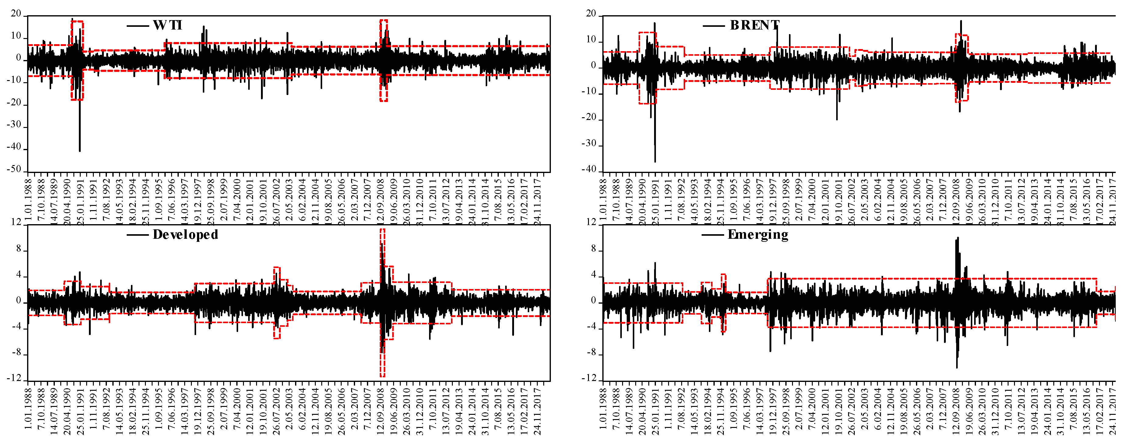
We first employ the modified IT statistic suggested by [16] to examine the existence of structural breaks in the variance of the return series. Figure 1 illustrates the return series with the structural break points and ± 3 standard deviations. We also present the dates of the detected structural breaks in the variance of the series in Table 2.
The IT test results suggest the existence of sudden change points (or, breaks) in the unconditional variance of all returns series. Specifically, we find seven sudden change points and 10 sudden change points for WTI and Brent oil price series, respectively. However, the MSCI emerging markets stock returns series have eight sudden changes points. The highest number of regime shifts points is detected for the MSCI G7 stock market returns series, where 13 structural breaks points are found.
3.2. Causality-In-Mean Tests
The studies in the literature indicate that the existence of structural breaks in the variance of series causes sharp size distortions in the causality-in-mean and variance tests. Therefore, the effects of structural breaks must be considered in Granger-causality tests. Following Lamoureux and Lastrapes [24], Aggarwal et al. [25], Arago-Manzana, and Fernandez-Izquierdo [26], Wang and Thi [27], Rapach and Strauss [28], and Ewing and Malik [29], we construct dummy variables to represent the structural breaks dates presented in Table 2. The dummy variables enter the variance equation as exogenous variables and account for the effects of the structural breaks.
To test for causal links among the crude oil and global stock markets, we first derive the standardized residuals from the respective EGARCH models and employ the causality-in-mean test procedure described earlier. The EGARCH estimates are presented in Table 3 (we present full model results in Appendix A). The results in Figure 1 show that some of the regime changes in the variance of developed and emerging stock markets are small. Hence, we examine whether the dummy variables representing the regime shifts are statistically significant and, as in Hammoudeh and Li [35] and Wang and Moore [36], we omit the statistically insignificant dummy variables in the final model estimation.
The optimal lag lengths for the autoregressive parameters in the EGARCH model’s mean equation are determined by means of several model information criteria, such as the Akaike Information Criterion (AIC), Hannan-Quinn criterion (HQ), and Schwarz’s Bayesian Information Criterion (SBIC). According to results in Table 3, the alpha (showing the size effect) and beta (showing the persistence effect) parameters are found to be statistically significant at the 1% level for all return series. The leverage parameter (γ) is negative and statistically significant at the 1% level for all return series—indicating that the effect of bad news on volatility is higher than the effect of good news in the crude oil and global stock markets. Also, the results in Table 3 show that the beta parameter, which indicates the degree of persistence in volatility in the EGARCH model, is significantly affected by structural breaks since we find a significant decrease in the beta parameter. These findings suggest that not accounting for the existence of structural breaks would have led to an upward bias in the estimated models’ parameters. Furthermore, the EGARCH models with the dummy variables are found to have higher log-likelihood values (and also lower model information criteria) than the EGARCH models without dummy variables, and these results suggest that returns series are better characterized by EGARCH models with structural breaks. A likelihood ratio (LR) test is employed to determine which model is more suitable in modeling the volatility of the return series, and the test results are also presented in Table 3 (the LR test can be calculated by using the formula, LR = 2[L(Md)−L(M)], where L(Md) and L(M) are the maximum log likelihood values derived from the EGARCH models with and without dummy variables, respectively). The LR test results provide evidence in favor of the EGARCH model with dummy variables since the null hypothesis can be rejected at a 1% significance level. These findings demonstrate that considering structural breaks in the EGARCH model estimation provides a better fit for volatility.
Based on the standardized residuals from the EGARCH models discussed above, the Granger-causality-in-mean test results are presented in Table 4. It is seen in Table 4 that only four out of the 10 possible causal relationships are statistically significant. It is further found that the WTI crude oil price changes are found to Granger-cause stock returns in emerging markets. In addition, we determine the existence of causality relation runs from stock market returns to Brent crude oil price changes. Furthermore, we find evidence for the presence of a unidirectional causal relationship from G7 stock markets to emerging stock markets. On the other hand, we cannot determine any Granger-causal links between the crude oil prices and G7 stock markets.
3.3. Causality-In-Variance Tests
Cheung and Ng [15] and Pantelidis and Pittis [37] showed that the existence of a causality-in-mean between the series might lead to the finding of spurious causality-in-variance if the effect is not considered in the test procedure. Therefore, we control for the causality-in-mean effects of crude oil (WTI and Brent) and the MSCI G7 stock markets on the MSCI emerging stock markets by including the lagged values of the respective crude oil and the MSCI G7 stock market returns series in the mean equation of the EGARCH model for the emerging stock market.
Next, we calculate the squares of the standardized GARCH residuals as the first step in the causality-in-variance test procedure. Note that the causality-in-variance between the series indicates the existence of volatility contagion effects. The results of the causality-in-variance tests are displayed in Table 5. We find the presence of causal links running from MSCI G7 stock returns to MSCI emerging stock returns and to Brent crude oil price changes. However, the test results suggest the lack of volatility spillover effects between the WTI crude oil price and the global stock market since the null hypothesis of no causality-in-variance cannot be rejected.
3.4. Time-Varying Causality-In-Mean Tests
The time-varying causality tests recognize the fact that the causal relationships between two (or more) variables can change overtime. In the context of the present paper, we employ the time-varying causality-in-mean and causality-in-variance tests to test whether the causal relationships (if any) between global crude oil price movements and the stock market returns in G7 countries and emerging markets changed over time.
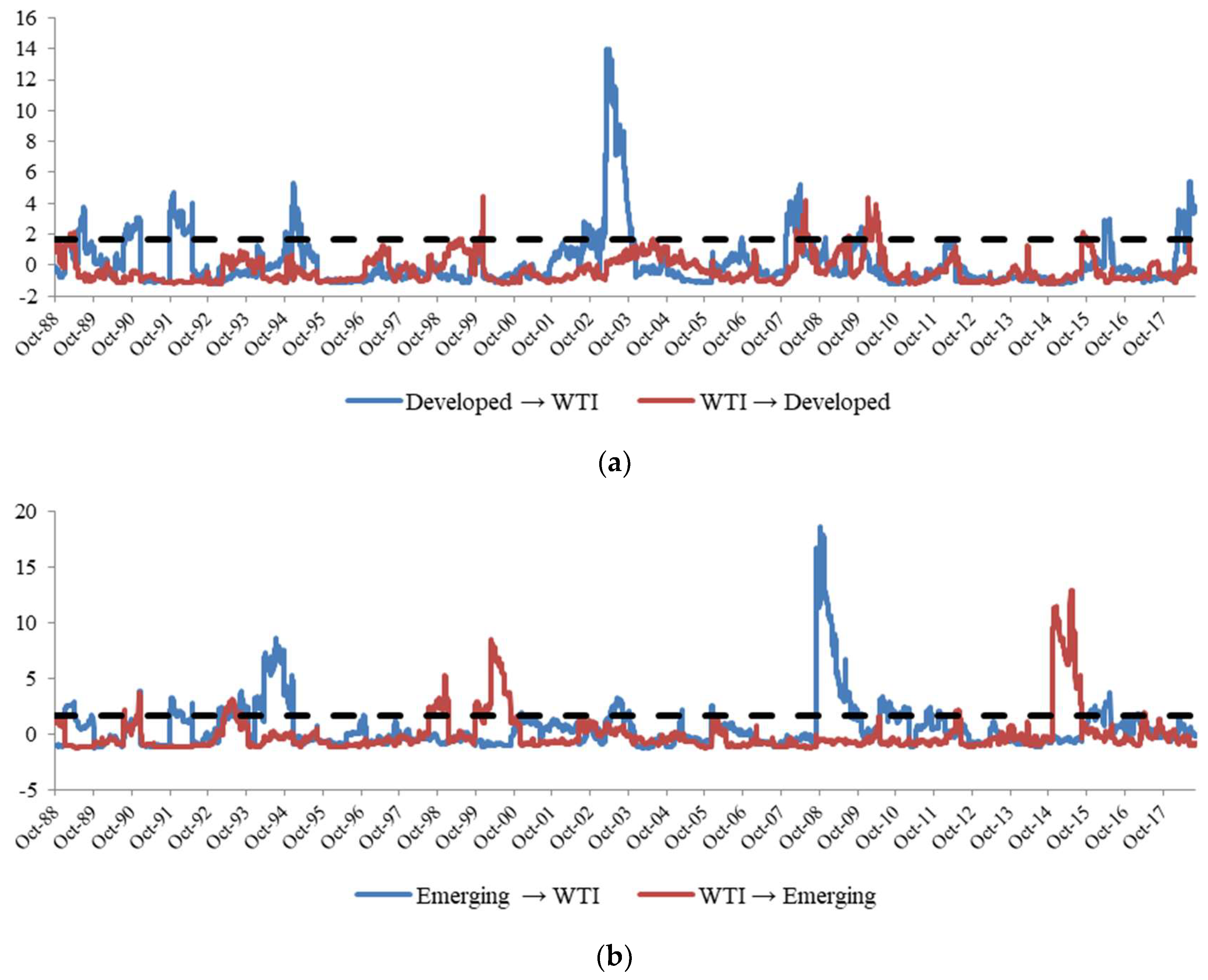
The test results for the causality-in-mean are presented in Figure 2. The results in Figure 2 indicate time-varying Granger-causal relationships in the mean between the crude oil prices and MSCI G7 and MSCI emerging markets stock returns and vice versa. This contrasts with the causality-in-mean test results in Table 4, which indicate that there is no causal link between the WTI crude oil price changes and MSCI G7 stock market returns. The non-time-varying Granger-causality tests represent an “on average” relationship and hence fail to account for the periods where a Granger-causal relationship might exit. The results in Panel (a) of Figure 2 show that there is a Granger-causal link running from the WTI crude oil price changes to MSCI G7 stock returns, especially during the global financial crisis. This finding is interesting because at the beginning of the global financial crisis, the G7 countries’ stock markets are affected by the developments in oil prices. Afterwards, the Granger-causal relationship was reversed. This finding is similar, but somewhat less strong, for the Granger-causal relationships between Brent crude oil prices and G7 stock market returns as seen in Panel (d) of Figure 2. In addition, we find evidence of short-lived Granger-causal links running from the crude oil price changes to G7 countries’ stock market returns at specific time periods, such as 1989, 1990–1991, 1993–1994, 2004, 2013, 2016, and 2017 (especially for Brent oil prices). These results, for instance, would not be detected by Granger-causality tests, which cover only the overall time period in reaching the conclusions. The time-varying causality test approach allows the detection of a causal relationship that prevails in sub-periods.
The results in Panel (b) of Figure 2 show that the Granger-causality generally runs from WTI crude oil price movements to the MSCI emerging stock market returns. This finding is consistent with the test results in Table 4. Specifically, the null hypothesis of “WTI crude oil price movements do not Granger cause emerging stock market returns” can be rejected more strongly in 1990 and this finding is consistent with a priori expectations because an unexpected oil price shock occurred at this time due to the Iraqi invasion of Kuwait. We also find evidence for the presence of a Granger-causal relationship between crude oil movements and MSCI emerging stock market returns during the global financial crisis.
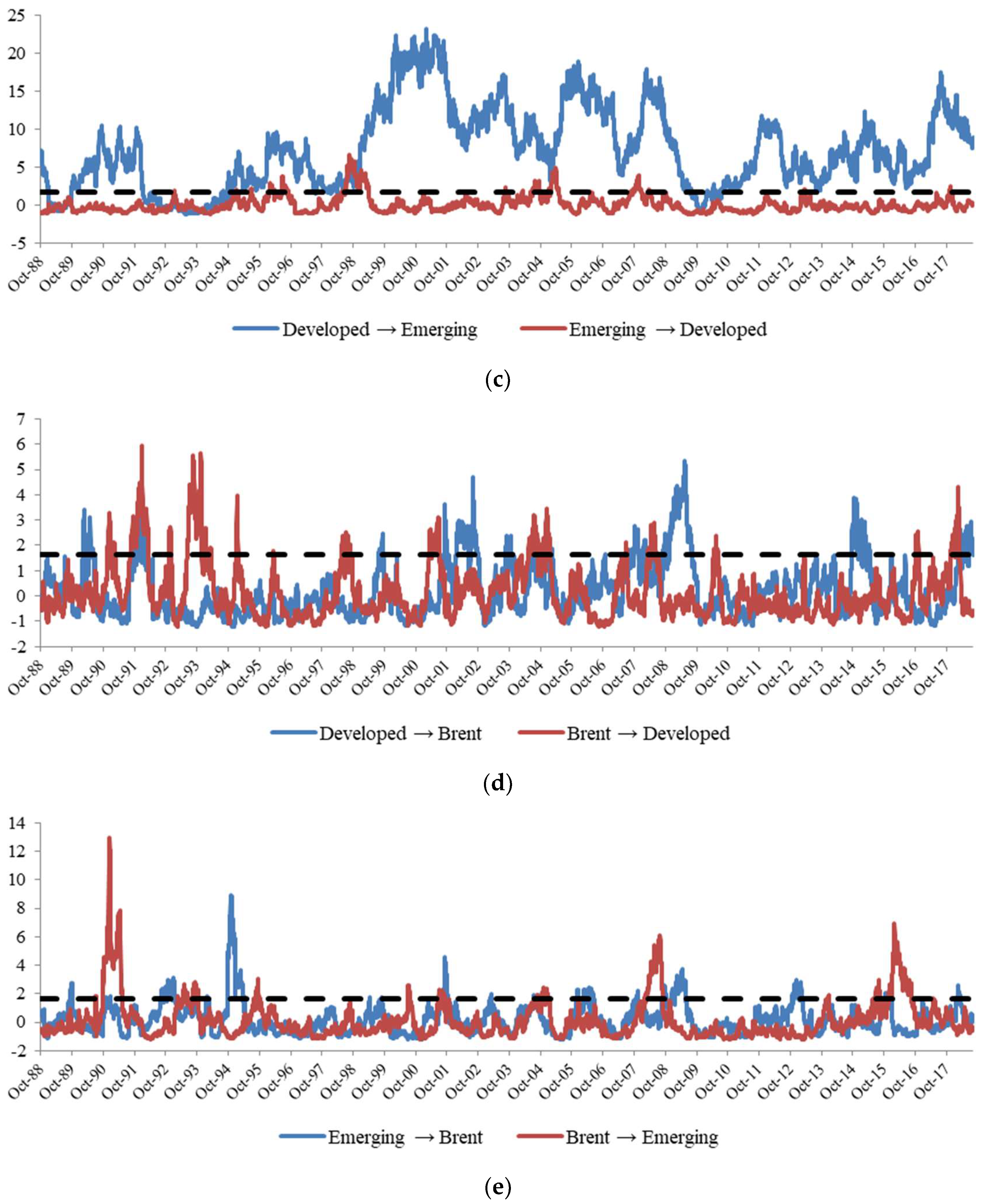
The results in Figure 2—Panel (c) indicate the existence of a Granger-causal relationship running from MSCI G7 stock market returns to MSCI emerging stock market returns. This finding is consistent with the causality-in-mean test results presented in Table 4. Furthermore, it can be said that the causal relationship running from G7 stock market returns to emerging stock market returns is stronger after 1998.
Panel (e) of Figure 2 displays the time-varying Granger-causal relationships between Brent crude oil price changes and MSCI emerging stock markets returns. There is evidence of a Granger-causal relationship in both directions. Nevertheless, developments in Brent oil prices appear to affect MSCI emerging stock market returns more strongly and frequently.
3.5. Time-Varying Granger-Causality-In-Variance Tests
The time-varying causality-in-variance test results are presented in Figure 3, Panels (a)—(e). The time-varying Granger-causality-in-variance test results in Table 5 indicate only the presence of a bidirectional Granger-causal relationship (feedback) between MSCI G7 and MSCI emerging stock markets. Nevertheless, the time-varying causality-in-variance test results provide us a different picture. Time-varying causality-in-variance test results indicate the presence of bidirectional causal links among the crude oil price changes (both WTI and Brent) and global stock market returns at specific time periods. For instance, we find evidence for the existence of volatility spillover effects from crude oil price changes to the MSCI G7 stock market returns in the 1990s, 2001, 2004, 2007–2008, 2013, 2015, and at the end of 2016. The Granger-causal volatility spillovers from Brent oil price developments and MSCI G7 stock markets’ returns draw a similar picture to the results from the WTI oil prices. Similarly, the test results suggest a Granger-causal volatility spillover link running from MSCI G7 stock markets’ returns to price changes in the WTI crude oil market in 1991–1992, 2001, 2004–2005, 2008–2009, and, most recently, from late-2017 till mid-2018. The volatility spillover effects from MSCI G7 stock returns to Brent oil price developments has somewhat stronger effects in the late 1980s, 1991, 1999, 2000–2003, 2007-2008, 2014, and in 2018. It is interesting to note that the Granger-causal effects turn out to be significant in most episodes of economic crises.
Panel (b) in Figure 3 indicates that there are volatility spillover effects from WTI crude oil price changes to MSCI emerging stock market returns in the late 1980s, 1990–1991, 1993, 1999, 2000–2001, 2007–2008, 2013–2014, and 2015–2017. We also find that return volatility in MSCI emerging stock markets Granger-cause the volatility of the WTI crude oil prices during the global financial crisis. The results in panel (c) show that the volatility spillover effects run mostly from MSCI G7 stock markets to MSCI emerging stock markets’ returns. Nevertheless, there is a period of feedback relationships as well. Note that the results in Table 5 indicate only unidirectional Granger-causality from MSCI G7 to MSCI emerging. Again, the time-varying Granger-causality tests shed more light into the understanding of the causal links between variables of interest.
3.6. Do the Granger-Causal Relationships between Oil Market Price Developments and Emerging Market Stock Returns Differ between Oil Exporting and Importing Countries?
In this sub-section, we investigate whether oil price developments affect oil-importing and oil-exporting countries’ stock markets differently (and vice versa). It might be the case that the relationship between stock market returns and crude oil market returns could be different for oil exporting and importing countries as an increase in oil prices could boost the stock markets in oil exporting countries while the opposite might arise for oil importing countries. Nevertheless, the net results are not clear since an increase (or decrease) in oil prices might also affect the overall global investment environment. Oil exporting emerging markets might appear to benefit from higher oil prices at first, but if the increase in oil prices leads to a negative macroeconomic environment elsewhere in the world, the oil exporting countries could also suffer from it in the long-term. The net effect is an empirical question and the analysis in this section attempts to shed some more light on it.
The MSCI Emerging Markets index used in our study includes 23 emerging markets’ countries, which can further be classified as oil exporting and oil importing countries. Therefore, we calculate two different emerging markets stock price indices, where the countries are classified as net oil exporting and importing. The oil exporting emerging market stock index covers the stock market indices of Brazil, Colombia, Mexico, Egypt, Russia, and Malaysia (we cannot consider Qatar and the United Arab Emirates (UAE) in calculating an index due to data availability. We cannot obtain the data for these countries before 2005). On the other hand, the oil importing emerging market stock index consists of the stock market index of 15 emerging markets. Due to data availability, we calculate the stock market indices for the period of 1 January 1994 to 27 August 2018. Next, we test for Granger-causal relationships between crude oil price changes (using both WTI and Brent oil prices) and stock market returns of oil exporting and importing countries. We employ the same methodology as discussed earlier. The results presented in Table 6 indicate that there is a bidirectional (feedback) relationship between Brent oil price changes and the stock market returns of oil importing and oil exporting countries. Hence, we find that there is no qualitative Granger-causal difference in the relationship between the oil-importing and oil-exporting emerging markets’ stock returns and Brent oil price changes. Nevertheless, we find that the WTI oil price changes unidirectionally Granger-cause the changes in the mean of the stock market returns. Stick market developments in oil-importing emerging markets do not Granger-cause the WTI oil price changes in mean. This might be arising since the Brent oil is more commonly used in oil-importing emerging markets than the WTI. A positive (negative) outlook in oil-importing emerging markets may not lead to increased (decreased) demand for WTI oil. In this context, Zhang and Chen [38], Dagher and El Hariri [39], and Jouini [40] and Bouri [11] found similar results and they showed the presence of a causal link between Brent oil price changes and stock market returns.
Table 7 presents the results from the Granger-causality-in-variance tests. We find that the only statistically significant Granger-causal volatility spillover is from WTI oil prices to the stock market returns of oil-importing countries. That is, increased (decreased) volatility in WTI oil prices lead to increased (decreased) volatility in the stock market returns of oil-importing countries. In combination with the results from Table 6, one can conclude that there is some difference between the effects of WTI oil price developments and Brent oil price developments on the stock market returns (both in mean and in terms of volatility) in oil-importing emerging markets.
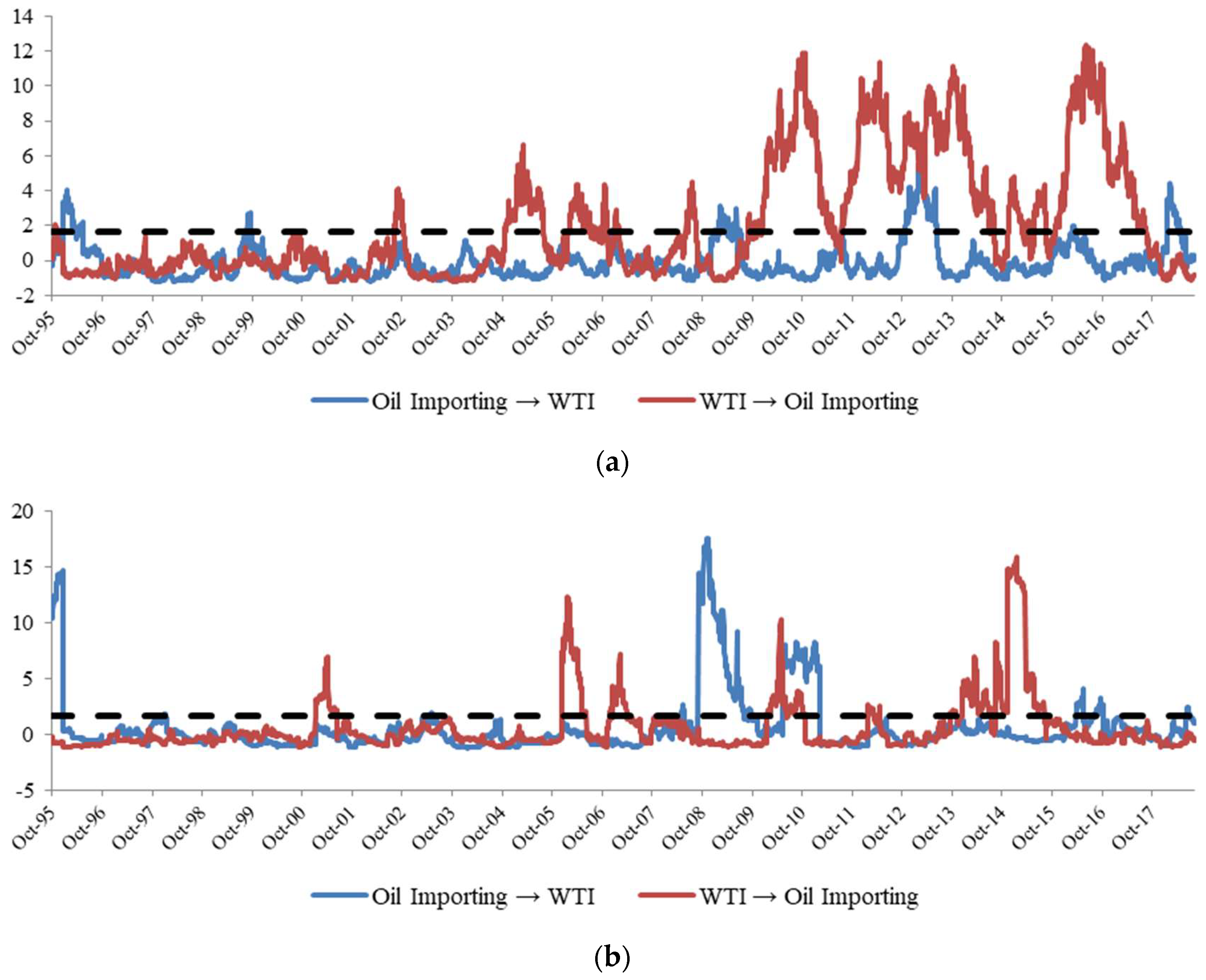
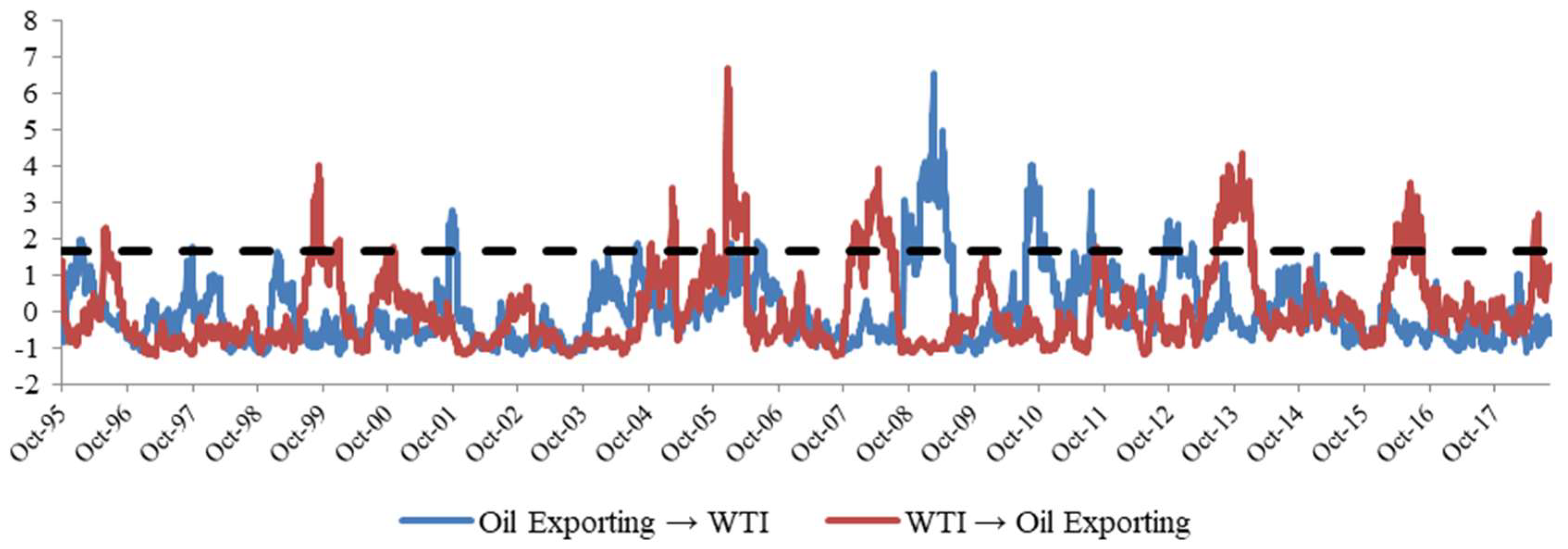
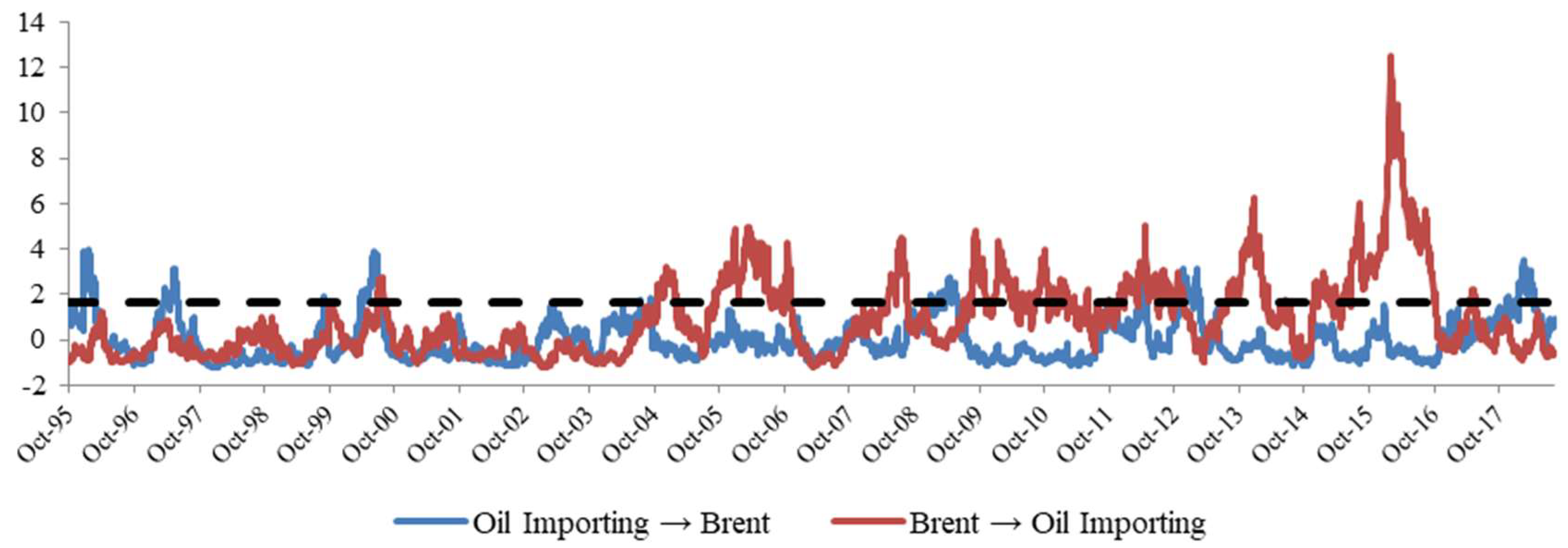
In understanding why this difference arises, we present the rolling-Granger-causality tests both for the means and the volatilities of the variables in question in Figure 4 Panels (a–b).
Figure 4—Panel (a) suggests that the changes in the WTI oil market prices had a more pronounced effect on oil-importing emerging markets’ stock markets in more recent periods—especially after the global financial crisis. With respect to the Granger-causality-in-variance or causal volatility spillover effects, some mixed evidence is seen in Figure 4—Panel (b). While the results in Table 7 do not indicate a Granger-causal link from oil-importing emerging market countries’ stock market volatility to the volatility of WTI oil prices, Figure 4—Panel (b) suggests that there is a time-varying nature in this relationship. Further investigation of the changing nature of the Granger-causal relationships in mean and in variance between the WTI oil price changes and oil-importing emerging markets’ stock market developments are left as part of a future research agenda. To be complete in our analysis, we present in Appendix B the results from the time-varying Granger-causality tests in mean and variance on the relationships between Brent oil prices and oil-importing and oil-exporting emerging markets’ stock market developments.
4. Discussion and Conclusions
This study investigates the causal relationships between price movements in crude oil markets (both WTI and Brent) and global stock returns by means of Cheung and Ng’s [15] and Hong’s [14] time-varying causality-in-mean and causality-in-variance tests. The analysis uses daily data covering the period from 1 January 1988 to 27 August 2018. The global stock markets were separated into two aggregate groups of countries, namely the MSCI developed (G7 countries) and MSCI emerging (23 emerging market countries). A further distinction was also made between oil-exporting and oil-importing emerging markets. Our results show that if one uses a causality test without taking the possible time-varying nature of the causal relationships, no causal link in-mean between oil prices and G7 stock markets would be detected. This is in line with the findings of Lee et al. [41]. In the case of emerging markets, we find a unidirectional causal link from oil prices to emerging countries’ stock markets. When it comes to the causality-in-variance test results, no causal linkages between oil prices and stock markets (both G7 and emerging markets) are found. Furthermore, it is found that stock market developments in the G7 countries have a unidirectional causal effect on emerging stock markets both in mean and in variance of the stock returns, which is in line with the earlier findings in the literature.
The time-varying (rolling) causality tests tell a more detailed and period-specific story. During the period from 1988 till the end of 1994, we find causal relationships running from crude oil to the global stock markets, and these results are consistent with theoretical expectations because at the beginning of the 1990s, the fluctuations in the crude oil price were high due to the Iraq invasion of Kuwait and the Iraq war. Therefore, the developments in the crude oil price affected the global stock market. However, there is no causal relationship between oil prices and global stock markets during the period from 1995 till the end of 2007. Specifically, the period of 2002–2007 represents the recovery and growth period after the early-2000s recession in the world economy. The oil prices increased substantially during this period from around USD 20 per barrel in 2002–2003 to above USD 100. The increase in oil prices is mainly attributed to the economic growth in the world economy while strategic oil reserve purchases by some countries, such as China and the US, may have contributed to some degree as well. The direction of the causal link between the G7 and the emerging stock markets tends to be a unilateral effect from the former to the latter.
The advantages of employing a time-varying framework to examine the nature of the causal relationships between oil prices and stock markets are best exemplified during and in the aftermath of the global financial crisis. It is found that (Figure 2, Panel (a)) there is bidirectional causality between oil prices and G7 stock markets in 2008 when the oil prices reached their maximum (about USD 150 in mid-2008). Nevertheless, real economic rates turned to negatives in G7 countries; this led to declines in oil prices, as well due to a weakened aggregate demand and industrial production and transportation. These results also highlight that the relationship between oil prices and stock markets might strongly depend on the phases of the economic cycles. In the aftermath of the 2008–2009 global financial crisis, the oil prices remained weak compared to pre-crisis times and there is no causal effect in any direction between oil prices and G7 stock market returns. This may represent a rather stable environment despite the continued worries about the health of the economies in developed countries.
On the emerging markets front, we find strong evidence in favor of a causality relationship from crude oil to emerging stock markets at the beginning of 1990s due to the First Gulf War. After that, we determine weak evidence in favor of a causal link between emerging stock markets and crude oil from 1992 till 2007 because the (non-) causality results are generally borderline cases. On the other hand, we find a bidirectional causal link between emerging markets and crude oil during the global financial crisis. In the post-global financial crisis period, however, there is more evidence of a causal link from oil prices to emerging markets stock prices. What is significantly different between the results from G7 and emerging markets is the presence of a strong unidirectional causal link from oil prices to emerging stock markets in 2013–2014 and in the period after 2015. We will re-evaluate these findings after discussing the results from the causality-in-variance tests.
The empirical findings from the causality-in-variance tests indicate the following: (1) During recession times, such as the early-1990s and 2000s and the global financial crisis, and during more recent concerns on economic growth in developed countries, there exists rather unidirectional causal volatility spillovers from G7 countries’ stock markets to crude oil prices. This finding can be explained by the increased uncertainty in the economic environment, leading to more uncertainty on future oil price developments. Although different in magnitude and the timing of the instances (periods), a similar conclusion can be reached regarding the causal link from the volatility of emerging markets’ stock returns to crude oil price volatility; (2) the analysis of the causal link from oil price volatility to G7 stock returns’ volatility indicates three episodes (1994, 1999, and 2007–2009) where there exists a causal relationship. Hence, it can be said that a feedback relationship is observed between the volatility in crude oil prices and stock price volatility during the global financial crisis (Figure 2, Panel (a)). A similar conclusion is not supported in the emerging markets. The causal effects are mainly from emerging stock markets’ return volatility to oil price volatility, notwithstanding the heightened probability of a causal feedback from oil price volatility to emerging stock markets’ return volatility, especially around 1998 and 2000. Nevertheless, what is a unique finding in the causal volatility spillovers’ analysis is that crude oil prices caused stock return volatility in emerging markets during the late-2014 to late-2015. This effect disappeared afterwards, but it is replaced by a higher probability of a causal link from the stock return volatility in emerging markets to oil price volatility. Increased oil price volatility in this period (see Figure 1) might be capturing both the geopolitical tensions in oil exporting countries (especially the Middle East and Venezuela) and the demand side uncertainty in emerging markets—given the concerns about the sustainability of higher growth rates in Asian economies; and (3) volatility spillovers from G7 stock markets to emerging markets’ stock returns show a unidirectional link in the period before the global financial crisis. This link breaks down in the post-crisis period and is replaced by a possibly weak feedback relationship more recently.
We also find that the there is no causally qualitative difference between the WTI crude oil price developments and Brent crude oil price developments on oil-exporting emerging markets’ countries’ stock returns and vice versa. Nevertheless, WTI oil prices have a unidirectional Granger-causal effect on oil-importing emerging markets’ stock returns both in mean and in variance. Time-varying Granger-causality test results suggest that the effect has become more pronounced in more recent periods after the global financial crisis.
Overall, our analysis shows that the importance of considering the changing nature of the causal links between stock returns and oil prices, and the additional information obtained by conducting the causality test not only for the mean of the series, but also for the variance of the series.
It must be recognized that our analysis is conducted in the aggregate stock returns for two groups of countries and the crude oil price changes. The literature provides examples of country specific results with additional sector-specific analysis as well. Nevertheless, given that the MSCI G7 and MSCI Emerging Markets indices are traded as aggregate indices in international financial markets, our results would provide insights to practitioners and professionals on how oil market price developments would affect their investments in these indices. Furthermore, since the stock market developments are considered to be a leading-indicator for economic activity, a better understanding of the time-varying nature of the volatility spillover relationships between oil prices and stock markets might help policy-makers in developed and developing countries in devising more effective policies to reduce financial market volatility and hence bring about more economic stability. Some options on the policy-making side may involve changes in the taxation of oil-based products, providing incentives for alternative energy generation projects to reduce dependence on oil, and providing incentives for the development and efficient functioning of future markets, especially in emerging markets, among others.
Author Contributions
Conceptualization, E.İ.Ç., E.A., and T.K.; Methodology, E.İ.Ç. and E.A.; Software, E.İ.Ç.; Formal Analysis, E.İ.Ç., E.A., and T.K.; Investigation, E.İ.Ç., E.A., and T.K.; Data Curation, E.İ.Ç.; Writing-Original Draft Preparation, E.İ.Ç. and E.A.; Writing-Review & Editing, E.İ.Ç., E.A., and T.K.; Overall, all authors contributed to the paper equally.
Funding
This research received no external funding.
Acknowledgments
An earlier version of this paper was presented at the International Congress of Energy and Economy and Security, Istanbul, Turkey, 25–26 March 2017. We thank the session participants and the discussant for their valuable comments and suggestions. We also thank two anonymous referees of Energies for their comments and suggestions on this paper that led to many improvements.
Conflicts of Interest
The authors declare no conflict of interest.
Appendix A. EGARCH Model with Dummy Variables

Table A1.
EGARCH model (with dummy variables) results.
| Parameters | WTI | Brent | Developed | Emerging |
|---|---|---|---|---|
| ω | −0.075 [0.000] | 0.001 [0.934] | −0.189 [0.000] | −0.143 [0.000] |
| α | 0.121 [0.000] | 0.121 [0.000] | 0.147 [0.000] | 0.184 [0.000] |
| β | 0.980 [0.000] | 0.900 [0.000] | 0.926 [0.000] | 0.961 [0.000] |
| γ | −0.021 [0.001] | −0.042 [0.000] | −0.136 [0.000] | −0.073 [0.000] |
| ν | 1.209 [0.000] | 1.217 [0.000] | 1.431 [0.000] | 1.454 [0.000] |
| d1 | 0.019 [0.001] | 0.038 [0.006] | 0.073 [0.000] | −0.0028 [0.008] |
| d2 | 0.048 [0.000] | 0.232 [0.000] | −0.012 [0.087] | -* |
| d3 | 0.022 [0.000] | −0.021 [0.064] | 0.062 [0.000] | −0.049 [0.000] |
| d4 | 0.016 [0.002] | 0.050 [0.002] | 0.155 [0.000] | -* |
| d5 | 0.066 [0.001] | 0.106 [0.000] | 0.103 [0.000] | −0.032 [0.008] |
| d6 | 0.008 [0.044] | 0.054 [0.000] | 0.081 [0.003] | -* |
| d7 | - | 0.218 [0.000] | -* | -* |
| d8 | - | 0.096 [0.005] | 0.071 [0.000] | - |
| d9 | - | 0.048 [0.046] | 0.263 [0.000] | - |
| d10 | - | −0.089 [0.000] | 0.163 [0.000] | - |
| d11 | - | 0.103 [0.000] | 0.067 [0.000] | - |
| d12 | - | - | -* | - |
| AIC | 4.245 | 4.118 | 2.197 | 2.626 |
| SBIC | 4.262 | 4.136 | 2.217 | 2.640 |
| HQ | 4.251 | 4.124 | 2.203 | 2.631 |
| Ln(L) | −16947.2 | −16447.9 | −8758.5 | −10480.0 |
| Q (50) | 54.135 [0.192] | 54.454 [0.212] | 55.944 [0.089] | 88.964 [0.000] |
| Qs (50) | 55.556 [0.158] | 87.791 [0.000] | 40.423 [0.831] | 61.559 [0.127] |
Note: The figures in square brackets show the p-values. v is a GED parameter. Q(50) and Qs(50) indicates the Ljung-Box serial correlation test values for the return and the squared return series, respectively. AIC, SBIC, and HQ indicate the Akaike, Schwarz, and Hannan-Quinn model information criteria, respectively. -* indicates deleted dummy variables that are found to be statistically insignificant.
Appendix B. Time-Varying Granger-Causality Tests between Crude Oil Market Developments and the Stock Market Returns in Oil-Exporting and Oil-Importing Emerging Markets
Figure A1.
Time-varying Granger-causality-in-mean test results between WTI oil prices and oil-exporting emerging markets’ stock returns.
Figure A1.
Time-varying Granger-causality-in-mean test results between WTI oil prices and oil-exporting emerging markets’ stock returns.

Figure A2.
Time-varying Granger-causality-in-mean test results between Brent oil prices and oil-exporting emerging markets’ stock returns.
Figure A2.
Time-varying Granger-causality-in-mean test results between Brent oil prices and oil-exporting emerging markets’ stock returns.

Figure A3.
Time-varying Granger-causality-in-mean test results between Brent oil prices and oil-importing emerging markets’ stock returns.
Figure A3.
Time-varying Granger-causality-in-mean test results between Brent oil prices and oil-importing emerging markets’ stock returns.

Figure A4.
Time-varying causality-in-variance test results between Brent oil prices and oil-importing emerging markets’ stock returns.
Figure A4.
Time-varying causality-in-variance test results between Brent oil prices and oil-importing emerging markets’ stock returns.

Figure A5.
Time-varying causality-in-variance test results between Brent oil prices and oil-exporting emerging markets’ stock returns.
Figure A5.
Time-varying causality-in-variance test results between Brent oil prices and oil-exporting emerging markets’ stock returns.

Figure A6.
Time-varying Granger-causality-in-variance test results between WTI oil prices and oil-exporting emerging markets’ stock returns.
Figure A6.
Time-varying Granger-causality-in-variance test results between WTI oil prices and oil-exporting emerging markets’ stock returns.

References
- Olowe, R.A. Oil price volatility, Global Financial Crisis, and the month-of-the-year effect. Int. J. Bus. Manag. 2010, 5, 156–170. [Google Scholar]
- Jones, C.M.; Kaul, G. Oil and the stock markets. J. Finance 1996, 51, 463–491. [Google Scholar] [CrossRef]
- Huang, B.D.; Masulis, R.W.; Stoll, H.R. Energy shocks and financial markets. J. Futur. Mark. 1996, 16, 1–27. [Google Scholar] [CrossRef]
- Sadorsky, P. Oil price shocks and stock market activity. Energy Econ. 1999, 21, 449–469. [Google Scholar] [CrossRef]
- Ciner, C. Energy shocks and financial markets: Nonlinear linkages. Stud. Non-Linear Dyn. Econ. 2001, 5, 203–212. [Google Scholar]
- Cong, R.-G.; Wei, Y.-M.; Jiao, J.-L.; Fan, Y. Relationships between oil price shocks and stock market: An empirical analysis from China. Energy Policy 2008, 36, 3544–3553. [Google Scholar] [CrossRef]
- Creti, A.; Ftiti, Z.; Guesmi, K. Oil price and financial markets: Multivariate dynamic frequency analysis. Energy Policy 2014, 73, 245–258. [Google Scholar] [CrossRef]
- Jimenez-Rodriguez, R. Oil price shocks and stock markets: Testing for nonlinearity. Empir. Econ. 2015, 48, 1079–1102. [Google Scholar] [CrossRef]
- La, T.-H.; Chang, Y. Effects of oil price shocks on the stock market performance: Do nature of shocks and economies matter? Energy Econ. 2015, 51, 261–274. [Google Scholar]
- Jammazi, R.; Nguyen, D.-K. Responses of international stock markets to oil price surges: A regime-switching perspective. Appl. Econ. 2015, 47, 4408–4422. [Google Scholar] [CrossRef]
- Bouri, E. A broadened causality in variance approach to assess the risk dynamics between crude oil prices and the Jordanian stock market. Energy Policy 2015, 85, 271–279. [Google Scholar] [CrossRef]
- Bastianin, A.; Conti, F.; Manera, M. The impacts of oil price shocks on stock market volatility: Evidence from the G7 countries. Energy Policy 2016, 98, 160–169. [Google Scholar] [CrossRef] [Green Version]
- Hamilton, J.D. What is an oil shock? J. Econ. 2003, 113, 363–398. [Google Scholar] [CrossRef]
- Hong, Y. A test for volatility spillover with application to exchange rates. J. Econ. 2001, 103, 183–224. [Google Scholar] [CrossRef]
- Cheung, Y.W.; Ng, L.K. A causality-in-variance test and its application to financial market prices. J. Econ. 1996, 72, 33–48. [Google Scholar] [CrossRef]
- Lu, F.; Hong, Y.; Wang, S.; Lai, K.; Liu, J. Time-varying Granger causality test for applications in global crude. Energy Econ. 2014, 42, 289–298. [Google Scholar] [CrossRef]
- Inclan, C.; Tiao, G.C. Use of cumulative sums of squares for retrospective detection of changes in variance. J. Am. Stat. Assoc. 1994, 89, 913–923. [Google Scholar]
- Sanso, A.; Arago, V.; Carrion, J.L. Testing for change in the unconditional variance of financial time series. Rev. De Econ. Financ. 2004, 4, 32–53. [Google Scholar]
- Chkili, W.; Hammoudeh, S.; Nguyen, D.K. Volatility forecasting and risk management for commodity markets in the presence of asymmetry and long memory. Energy Econ. 2014, 41, 1–18. [Google Scholar] [CrossRef]
- Klein, T.; Walther, T. Oil price volatility forecast with mixture memory GARCH. Energy Econ. 2016, 58, 46–58. [Google Scholar] [CrossRef]
- Nelson, D.B. Conditional heteroskedasticity in asset returns: A new approach. Econometrica 1991, 59, 347–370. [Google Scholar] [CrossRef]
- Van Belle, G. Statistical Rules of Thumb, 2nd ed.; John Wiley & Sons: Hoboken, NJ, USA, 2008; ISBN 978-0-470-14448-0. [Google Scholar]
- Hillebrand, E. Neglecting parameter changes in GARCH models. J. Econ. 2005, 129, 121–138. [Google Scholar] [CrossRef]
- Lamoureux, C.G.; Lastrapes, W.D. Persistence in variance, structural change and the GARCH model. J. Bus. Econ. Stat. 1990, 68, 225–234. [Google Scholar]
- Aggarwal, R.; Inclan, C.; Leal, R. Volatility in emerging markets. J. Financ. Quant. Anal. 1999, 34, 33–55. [Google Scholar] [CrossRef]
- Arago-Manzana, V.; Fernandez-Izquierdo, M.A. Influence of structural changes in transmission of information between stock markets: A European empirical study. J. Multinatl. Financ. Manag. 2007, 17, 112–124. [Google Scholar] [CrossRef]
- Wang, K.-M.; Thi, T.-B.N. Testing for contagion under asymmetric dynamics: Evidence from the stock markets between US and Taiwan. Physica A 2007, 376, 422–432. [Google Scholar] [CrossRef]
- Rapach, D.E.; Strauss, J.K. Structural breaks and GARCH models of exchange rate volatility. J. Appl. Econ. 2008, 23, 65–90. [Google Scholar] [CrossRef]
- Ewing, B.T.; Malik, F. Estimating volatility persistence in oil prices under structural breaks. Financ. Rev. 2010, 45, 1011–1023. [Google Scholar] [CrossRef]
- Walther, T.; Klein, T.; Thu, H.P.; Piontek, K. True or spurious long memory in European non-EMU currencies. Res. Int. Bus. Finance 2017, 40, 217–230. [Google Scholar] [CrossRef]
- Charfeddine, L. True or spurious long memory in volatility: Further evidence on the energy futures markets. Energy Policy 2014, 71, 76–93. [Google Scholar] [CrossRef]
- Javed, F.; Mantalos, P. Sensitivity of the causality in variance test to the GARCH (1, 1) parameters. Child. J. Stat. 2015, 6, 49–65. [Google Scholar] [CrossRef]
- Van Dijk, D.; Osborn, D.R.; Sensier, M. Testing for causality in variance in the presence of breaks. Econ. Lett. 2005, 89, 193–199. [Google Scholar] [CrossRef] [Green Version]
- Rodrigues, P.M.M.; Rubia, A. Testing for causality in variance under nonstationarity in variance. Econ. Lett. 2007, 97, 133–137. [Google Scholar] [CrossRef]
- Hammoudeh, S.; Li, H. Sudden changes in volatility in emerging markets: The case of Gulf Arab stock markets. Int. Rev. Financ. Anal. 2008, 17, 47–63. [Google Scholar] [CrossRef]
- Wang, P.; Moore, T. Sudden changes in volatility: The case of five central European stock markets. J. Int. Financ. Mark. Inst. Money 2009, 19, 33–46. [Google Scholar] [CrossRef] [Green Version]
- Pantelidis, T.; Pittis, N. Testing for Granger causality in variance in the presence of causality in mean. Econ. Lett. 2004, 85, 201–207. [Google Scholar] [CrossRef]
- Zhang, C.; Chen, X. The impact of global oil price shocks on China’s stock returns: Evidence from the ARJI(-ht)-EGARCH model. Energy 2011, 36, 6627–6633. [Google Scholar] [CrossRef]
- Dagher, L.; El Hariri, S. The impact of global oil price shocks on the Lebanese stock market. Energy 2013, 63, 366–374. [Google Scholar] [CrossRef]
- Jouini, J. Return and volatility interaction between oil prices and stock markets in Saudi Arabia. J. Policy Model. 2013, 35, 1124–1144. [Google Scholar] [CrossRef]
- Lee, B.-J.; Yang, C.W.; Huang, B.-N. Oil price movements and stock markets revisited: A case of sector stock price indexes in the G-7 countries. Energy Econ. 2012, 34, 1284–1300. [Google Scholar] [CrossRef]
Figure 1.
Daily returns series of West Texas Intermediate (WTI) crude oil prices, Brent crude oil prices, Morgan Stanley Capital International (MSCI) G7 stock prices, and MSCI emerging stock prices.
Figure 1.
Daily returns series of West Texas Intermediate (WTI) crude oil prices, Brent crude oil prices, Morgan Stanley Capital International (MSCI) G7 stock prices, and MSCI emerging stock prices.

Figure 2.
(a) Time-varying Granger-causality-in-mean test results between WTI oil prices and MSCI G7 stock returns. (b) Time-varying Granger-causality-in-mean test results between WTI oil prices and MSCI emerging markets’ stock returns. (c) Time-varying Granger-causality-in-mean test results between MSCI G7 and MSCI emerging markets’ stock returns. (d) Time-varying Granger-causality-in-mean test results between Brent oil prices and MSCI G7 stock returns. (e) Time-varying Granger-causality-in-mean test results between Brent oil prices and MSCI emerging markets’ stock returns.


Figure 3.
(a) Time-varying Granger-causality-in-variance test results between WTI oil prices and MSCI G7 stock returns. (b). Time-varying Granger-causality-in-variance test results between WTI oil prices and MSCI emerging markets’ stock returns. (c) Time-varying Granger-causality-in-variance test results between MSCI G7 and MSCI emerging markets’ stock returns. (d) Time-varying Granger-causality-in-variance test results between Brent oil prices and MSCI G7 stock returns. (e) Time-varying Granger-causality-in-mean test results between Brent oil prices and MSCI emerging markets’ stock returns.


Figure 4.
(a) Time-varying Granger-causality-in-mean test results between WTI oil prices and oil-importing emerging markets’ stock returns. (b) Time-varying Granger-causality-in-mean test results between WTI oil prices and oil-exporting emerging markets’ stock returns.
Figure 4.
(a) Time-varying Granger-causality-in-mean test results between WTI oil prices and oil-importing emerging markets’ stock returns. (b) Time-varying Granger-causality-in-mean test results between WTI oil prices and oil-exporting emerging markets’ stock returns.

Table 1.
Descriptive statistics.
| Statistics | WTI | Brent | Developed | Emerging |
|---|---|---|---|---|
| n | 7997 | 7997 | 7997 | 7997 |
| Mean | 0.017 | 0.018 | 0.020 | 0.059 |
| Std. Dev. | 2.409 | 2.242 | 0.912 | 1.116 |
| Skewness | −0.711 | −0.571 | −0.361 | −0.556 |
| Kurtosis | 18.211 | 17.301 | 11.272 | 10.782 |
| Jarque-Bera | 77766 [0.000] | 68586 [0.000] | 22975 [0.000] | 20594 [0.000] |
| ARCH (5) | 71.974 [0.000] | 108.77 [0.000] | 477.84 [0.000] | 414.22 [0.000] |
| Q (20) | 52.480 [0.000] | 50.303 [0.000] | 149.734 [0.000] | 549.616 [0.000] |
| Qs (20) | 838.795 [0.000] | 956.540 [0.000] | 10778.9 [0.000] | 9761.13 [0.000] |
| ADF | −34.823 *** | −20.617 *** | −20.920 *** | −13.504 *** |
| PP | −91.623 *** | −86.680 *** | −80.958 *** | −70.405 *** |
| KPSS | 0.039 *** | 0.047 **** | 0.059 *** | 0.075 *** |
Notes: The figures in square brackets show the probability (p-values) of rejecting the null hypothesis. ARCH (5) indicates an LM conditional variance test. Q(20) and Qs(20) indicate the Ljung-Box serial correlation test for returns and squared returns series, respectively. *** indicate that the series in question is stationary at the 1% significance level.
Table 2.
Variance break tests results.
| Series | No. of Breaks | Break Dates | ||||||
|---|---|---|---|---|---|---|---|---|
| WTI | 7 | 31.7.1990 | 22.3.1991 | 25.11.1991 | 8.1.1996 | 26.6.2003 | 12.09.2008 | 27.01.2009 |
| Brent | 12 | 31.7.1990 | 19.3.1991 | 8.1.1996 | 13.3.1998 | 18.4.2002 | 20.8.2008 | 2.4.2009 |
| 6.10.2009 | 26.08.2010 | 19.11.2012 | 27.11.2014 | 1.12.2016 | - | - | ||
| MSCI G7 Stock Index | 13 | 19.2.1990 | 11.2.1991 | 13.10.1992 | 16.10.1997 | 14.6.2002 | 17.10.2002 | 2.4.2003 |
| 22.7.2003 | 23.7.2007 | 12.9.2008 | 8.12.2008 | 3.6.2009 | 19.11.2012 | - | ||
| MSCI Emerging Stock Index | 8 | 31.8.1992 | 7.10.1993 | 19.5.1994 | 19.12.1994 | 14.3.1995 | 27.8.1997 | 15.12.2016 |
| 29.01.2018 | - | - | - | - | - | - | ||
Table 3.
EGARCH model results.
| Parameters | WTI | Brent | Developed | Emerging | ||||
|---|---|---|---|---|---|---|---|---|
| Without Dummies | With Dummies | Without Dummies | With Dummies | Without Dummies | With Dummies | Without Dummies | With Dummies | |
| ω | −0.078 [0.000] | −0.075 [0.000] | −0.072 [0.000] | 0.001 [0.934] | −0.116 [0.000] | −0.189 [0.000] | −0.146 [0.000] | −0.143 [0.000] |
| α | 0.124 [0.000] | 0.121 [0.000] | 0.111 [0.000] | 0.121 [0.000] | 0.136 [0.000] | 0.147 [0.000] | 0.185 [0.000] | 0.184 [0.000] |
| β | 0.991 [0.000] | 0.980 [0.000] | 0.993 [0.000] | 0.900 [0.000] | 0.982 [0.000] | 0.926 [0.000] | 0.976 [0.000] | 0.961 [0.000] |
| γ | −0.018 [0.001] | −0.021 [0.001] | −0.017 [0.000] | −0.042 [0.000] | −0.100 [0.000] | −0.136 [0.000] | −0.063 [0.000] | −0.073 [0.000] |
| ν | 1.191 [0.000] | 1.209 [0.000] | 1.181 [0.000] | 1.217 [0.000] | 1.391 [0.000] | 1.431 [0.000] | 1.444 [0.000] | 1.454 [0.000] |
| AIC | 4.248 | 4.245 | 4.129 | 4.118 | 2.210 | 2.197 | 2.630 | 2.626 |
| SBIC | 4.260 | 4.262 | 4.137 | 4.136 | 2.221 | 2.217 | 2.641 | 2.640 |
| HQ | 4.252 | 4.251 | 4.131 | 4.124 | 2.214 | 2.203 | 2.634 | 2.631 |
| Ln(L) | −16963.4 | −16947.2 | −16501.8 | −16447.9 | −8821.2 | −8758.5 | −10499.8 | −10480.0 |
| Q (50) | 52.471 [0.129] | 54.135 [0.192] | 53.860 [0.228] | 54.454 [0.212] | 50.801 [0.193] | 55.944 [0.089] | 89.947 [0.000] | 88.964 [0.000] |
| Qs (50) | 56.720 [0.239] | 55.556 [0.158] | 107.94 [0.000] | 87.791 [0.000] | 41.175 [0.809] | 40.423 [0.831] | 53.619 [0.337] | 61.559 [0.127] |
| LR | 32.54 [0.000] | 107.8 [0.000] | 125.40 [0.000] | 39.60 [0.000] | ||||
Note: The figures in square brackets show the p-values. v is a GED parameter. Q (50) and Qs (50) indicates the Ljung-Box serial correlation test values for the return and the squared return series, respectively. AIC, SBIC, and HQ indicate the Akaike, Schwarz, and Hannan-Quinn model information criteria respectively. Please see Appendix A for the full model estimates with dummy variables.
Table 4.
Granger-causality-in-mean test results.
| Granger-Causality Direction | M = 1 | M = 2 | M = 3 | M = 4 | M = 5 |
|---|---|---|---|---|---|
| WTI → MSCI G7 | −0.023 | 0.115 | 0.136 | 0.103 | 0.198 |
| MSCI G7 → WTI | 1.270 | 1.142 | 0.958 | 0.780 | 0.621 |
| Brent → MSCI G7 | −0.638 | −0.544 | −0.508 | −0.332 | −0.062 |
| MSCI G7 → Brent | 6.865 *** | 6.885 *** | 6.606 *** | 6.227 *** | 5.836 *** |
| WTI → MSCI Emerging | 5.338 *** | 5.362 *** | 5.088 *** | 4.729 *** | 4.375 *** |
| MSCI Emerging → WTI | 0.634 | 0.445 | 0.501 | 0.704 | 0.929 |
| Brent → MSCI Emerging | 0.758 | 0.860 | 0.836 | 0.739 | 0.619 |
| MSCI Emerging→ Brent | 3.884 *** | 3.636 *** | 3.385 *** | 3.171 *** | 2.992 *** |
| MSCI G7 → MSCI Emerging | 315.743 *** | 309.279 *** | 292.120 *** | 274.590 *** | 258.822 *** |
| MSCI Emerging → MSCI G7 | 0.176 | 0.032 | −0.059 | −0.065 | 0.078 |
Note: *** and ** indicates the existence of a causal link at the 1% and 5% significance level, respectively. M represents the maximum lag.
Table 5.
Causality-in-variance test results.
| Causality Direction | M = 1 | M = 2 | M = 3 | M = 4 | M = 5 |
|---|---|---|---|---|---|
| WTI → MSCI G7 | 1.145 | 0.951 | 0.780 | 0.633 | 0.547 |
| MSCI G7 → WTI | 0.040 | 0.342 | 0.470 | 0.520 | 0.571 |
| Brent → MSCI G7 | −0.696 | −0.841 | −0.961 | −0.988 | −0.968 |
| MSCI G7 → Brent | −0.483 | 1.813 ** | 3.318 *** | 4.047 *** | 4.398 *** |
| WTI → MSCI Emerging | −0.660 | −0.811 | −0.953 | −1.076 | −1.167 |
| MSCI Emerging → WTI | −0.208 | −0.026 | 0.119 | 0.175 | 0.209 |
| Brent → MSCI Emerging | 1.399 * | 1.211 | 0.961 | 0.725 | 0.638 |
| MSCI Emerging→ Brent | −0.438 | 0.049 | 0.695 | 1.163 | 1.409 * |
| MSCI G7 → MSCI Emerging | 3.599 *** | 4.184 *** | 4.361 *** | 4.339 *** | 4.305 *** |
| MSCI Emerging → MSCI G7 | −0.548 | −0.696 | −0.720 | −0.715 | −0.738 |
Note: ***, **, and * indicate the existence of a causal link at the 1%, 5%, and 10% significance level, respectively. M represents the maximum lag.
Table 6.
Granger-causality-in-mean test results.
| Causality Direction | M = 1 | M = 2 | M = 3 | M = 4 | M = 5 |
|---|---|---|---|---|---|
| Brent → Oil Exporting | 2.640 *** | 2.568 *** | 2.402 *** | 2.285 ** | 2.187 ** |
| Oil Exporting → Brent | 8.125 *** | 7.795 *** | 7.177 *** | 6.599 *** | 6.101 *** |
| Brent → Oil Importing | 18.063 *** | 17.360 *** | 16.082 *** | 14.864 *** | 13.803 *** |
| Oil Importing → Brent | 3.114 *** | 2.905 *** | 2.701 *** | 2.537 *** | 2.386 *** |
| WTI → Oil Exporting | 3.928 *** | 3.816 *** | 3.538 *** | 3.312 *** | 3.130 *** |
| Oil Exporting → WTI | 2.544 ** | 2.303 ** | 1.977 ** | 1.777 ** | 1.687 ** |
| WTI → Oil Importing | 31.553 *** | 30.582 *** | 28.586 *** | 26.635 *** | 24.906 *** |
| Oil Importing → WTI | −0.253 | −0.189 | 0.014 | 0.225 | 0.403 |
Note: *** and ** indicates the existence of a causal link at the 1% and 5% significance level, respectively. M represents the maximum lag.
Table 7.
Granger-causality-in-variance test results.
| Causality Direction | M = 1 | M = 2 | M = 3 | M = 4 | M = 5 |
|---|---|---|---|---|---|
| Brent → Oil Exporting | −0.550 | −0.532 | −0.560 | −0.627 | −0.708 |
| Oil Exporting → Brent | −0.691 | −0.818 | −0.898 | −0.968 | −1.031 |
| Brent → Oil Importing | 1.580 | 1.367 | 1.219 | 1.114 | 1.057 |
| Oil Importing → Brent | −0.392 | −0.464 | −0.568 | −0.684 | −0.612 |
| WTI → Oil Exporting | −0.607 | −0.760 | −0.908 | −1.029 | −1.131 |
| Oil Exporting → WTI | −0.523 | −0.551 | −0.610 | −0.691 | −0.723 |
| WTI → Oil Importing | 3.759 *** | 3.623 *** | 3.397 *** | 3.155 *** | 2.910 *** |
| Oil Importing → WTI | −0.704 | −0.757 | −0.833 | −0.850 | −0.748 |
Note: *** and ** indicates the existence of a causal link at the 1% and 5% significance level, respectively. M represents the maximum lag.
© 2018 by the authors. Licensee MDPI, Basel, Switzerland. This article is an open access article distributed under the terms and conditions of the Creative Commons Attribution (CC BY) license (http://creativecommons.org/licenses/by/4.0/).
Share and Cite
MDPI and ACS Style
Çevik, E.İ.; Atukeren, E.; Korkmaz, T. Oil Prices and Global Stock Markets: A Time-Varying Causality-In-Mean and Causality-in-Variance Analysis. Energies 2018, 11, 2848. https://doi.org/10.3390/en11102848
AMA Style
Çevik Eİ, Atukeren E, Korkmaz T. Oil Prices and Global Stock Markets: A Time-Varying Causality-In-Mean and Causality-in-Variance Analysis. Energies. 2018; 11(10):2848. https://doi.org/10.3390/en11102848
Chicago/Turabian StyleÇevik, Emrah İ., Erdal Atukeren, and Turhan Korkmaz. 2018. "Oil Prices and Global Stock Markets: A Time-Varying Causality-In-Mean and Causality-in-Variance Analysis" Energies 11, no. 10: 2848. https://doi.org/10.3390/en11102848
Note that from the first issue of 2016, this journal uses article numbers instead of page numbers. See further details here.