Differential Steering Control of Four-Wheel Independent-Drive Electric Vehicles

Abstract

This paper investigates the skid steering of four-wheel independent-drive (4WID) electric vehicles (EV) and a differential steering of a 4WID EV with a steer-by-wire (SBW) system in case of steering failure. The dynamic models of skid steering vehicle (SSV) and differential steering vehicle (DSV) are established and the traditional front-wheel steering vehicle with neutral steering characteristics is selected as the reference model. On this basis, sideslip angle observer and two different sliding mode variable structure controllers for SSV and DSV are designed respectively. Co-simulation results of CarSim and Simulink show that the designed controller for DSV not only controls the yaw rate and sideslip angle of DSV to track those of the reference model exactly, but also ensures the robustness of the controlled system compared with the designed controller for SSV. And the differential driving torque needed to realize the differential steering is much smaller than that for skid steering, which indicates the possibility of the differential steering in case of steering failure.

1. Introduction

The vehicle steering system has experienced several stages, such as manual steering, hydraulic steering, electro-hydraulic steering, electric power steering and by-wire steering. However, in order to achieve the latter two, the structure becomes more complicated because one or two extra motors are required [1]. The appearance of four-wheel independent-drive (4WID) electric vehicles (EVs) opens up the possibility of differential steering system (DSS) by coupled control of left and right in-wheel motors (IWM), which eliminates the restrictions of a traditional steering system completely [2]. With the emergence of intelligent vehicle systems (IVS), the 4WID system can also be used to solve the path tracking problem [3,4]. However, there are three functions of the DSS: (1) Steering the vehicle without the lateral turning of the wheel, i.e., skid steering [5,6]; (2) Assisting the driver to steer the vehicle, that is, differential drive assisted steering (DDAS) [1,2,7,8]; (3) Steering the vehicle instead of the regular steering system [9,10,11,12,13]. Skid steering was realized by giving a tire speed differential between the left and right tires [5,6]. And the wheel torque difference between the left and right tires, which controlled the tire velocity difference, was defined as a function of the steering wheel angle. In addition, a stability compensator for the adhesion limit of tire/load and the yaw rate and yaw acceleration are used as control variables. However, the needed differential driving torque is not given in the paper [5].

A closed loop control method of differential drive assisted steering (DDAS) was proposed, which includes a reference steering wheel torque (RSWT) design module and an integral anti-windup variable PI control module. The former was to design a three-dimensional characteristic curve of torque and steering wheel angle at different vehicle speeds, and the latter was aiming to address the saturation of motor’s output torque. The simulation results showed that the RSWT can be tracked perfectly by the DDAS, drivers’ handling efforts were reduced and the vehicle steering performance was improved [1]. A multidiscipline collaborative optimization model of the differential steering system was built with the steering economy as the main system, and the steering flexibility, the steering road feel and the mechanic character of the steering sensors as the subsystems. And the main system and the subsystems were optimized by the multi-island algorithm and the sequential quadratic programming algorithm. The simulation results show that the differential steering system can have good economy, good steering road feel, good steering flexibility and good mechanic character of the steering sensors [2]. The DDAS control system, the drive torque distribution and the compensation control system were designed. The proportional–integral (PI) feedback control loop was employed to track the reference steering effort. In addition, the traction control subsystem and the direct yaw moment control subsystem were both employed to make the DDAS work as well as wished [7]. The structure and basic theory of the DSS were discussed and its dynamic model was built. A H_∞ mixed sensitivity controller is designed to suppress the model uncertainties and road disturbance. The simulation results verified the efficacy of the DSS with the designed controller [8]. However, they are aimed at mitigating the driver’s steering efforts.

By regulating the four wheels to the desired differential speed base on the reference vehicle velocity, kinematic model of the distributed wheels, combined with Ackermann–Jeant and steering model, was introduced to achieve electrical differential steering for 4WID EVs. The effectiveness of the proposed control strategy was demonstrated by the simulation and experimental study [9]. A continuous steering stability controller based on energy-saving torque distribution algorithm was proposed for four-wheeled built-in motor independent driving electric vehicle. The simulation results showed that, compared with the traditional servo controller and the ordinary continuous controller, the proposed controller can significantly reduce the energy consumption and improve the steering stability of the vehicle [10]. The literature [11,12,13] investigates the DSS in the case of the complete failure of the regular steering system. To achieve the yaw stabilization, a robust H_∞ output-feedback controller of the DSS was designed and parametric uncertainties for the cornering stiffness and the external disturbances were considered to guarantee the vehicle robustness [11]. A multiple-disturbances observer-based composite nonlinear feedback (CNF) approach was proposed to improve the transient performance of the fault-tolerant control with the DDAS, and the disturbance observer was designed to estimate the external disturbances with unknown bounds. CarSim-Simulink joint simulation results verified the efficacy of the proposed controller [12]. To realize the yaw control when the active front steering entirely breaks down and guarantee the transient control performance, a disturbance observer based integral sliding mode control (ISMC) strategy was designed to deal with the unknown mismatched disturbances, which was addressed by an adaptive super-twisting control approach. And the composite nonlinear feedback technique was applied to design the controller’s nominal part to depress overshoots and avoid steady-state errors considering the tire force saturations. The simulation results verified the effectiveness of the proposed control approach in the case of the steering failure [13].

The innovation points are as follows: (1) Based on the reference model, the steering function of SSV and DSV are realized by the differential driving torque between the two sides of the front wheels instead of the normal desired differential speed; (2) An simple and practicable observer is constructed to estimate the actual sideslip angle; (3) The vehicle has parametric uncertainties, such as tire stiffness perturbation and external disturbances, and there is no direct relationship between handling wheel angle and differential driving torque of the left and right side wheels, thus two kinds of SMC controller are designed; (4) Contrast and analysis of the SSV and the DSV with controllers is carried out, such as the response curves, the needed differential torque and robustness.

The article structure is as follows: The SSV and DSV models, and reference model are described in Section 2. Sideslip angle observer and two kinds of SMC controller based on the reference model are designed in Section 3. Section 4 is the joint simulation based on CarSim (MATLAB, R2012a, mathworks, Natick, MA, USA) and Simulink. (CarSim, 8.02, MSC software, Los Angeles, CA, USA) Section 5 is the conclusion.

2. Vehicle Models and Problem Formulation

In this section, we will first present three kinds of vehicle models, including an SSV model, a DSV model and a reference model. Here vehicle models are based on the following assumptions: (1) The lateral acceleration is small and the roll motion can be ignored; (2) The left and right tire slip angles are equal; (3) The front and rear tire lateral forces are proportional to the tire slip angles. Then the problem formulation will be proposed.

The difference between SSV and DSV is that the former has no mechanical steering mechanism. However, both of them depend on the differential driving torque between the two sides of front wheels, but for the latter, the torque will also contribute to the generation of the front wheel angles. The SSV obtains steering yaw moment by increasing the speed of outer wheels and decreasing the speed of inner wheels, other than swinging the steered wheels.

2.1. Skid Steering Vehicle Model

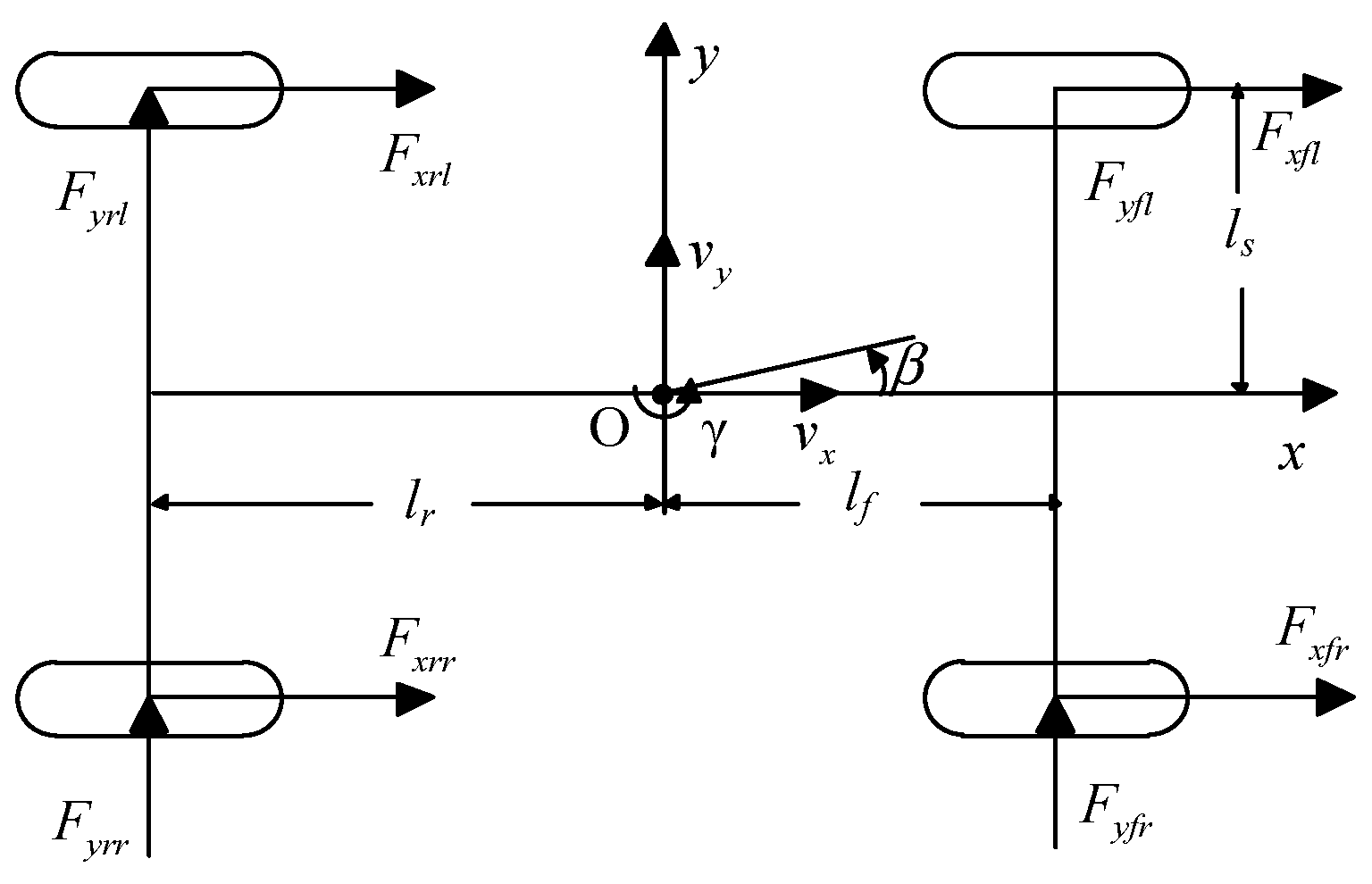
The forces acting on the vehicle body are shown in Figure 1, where F_xij (i = f,r, j = l,r) is the tire longitudinal force of the left/right front/rear wheel, F_yij (i = f,r, j = l,r) is the tire lateral force of the left/right front/rear wheel.

The lateral and yaw motion of the EV are modeled as:

$$\{\begin{array}{l}m{u}_x(\dot{\beta }+\gamma )=F_{yfl}+F_{yfr}+F_{yrl}+F_{yrr}\\ I_Z\dot{\gamma }=l_s\frac{\Delta M}{R}+l_f(F_{yfl}+F_{yfr})-l_r(F_{yrl}+F_{yrr})\end{array}$$

(1)

where

$$F_{yfl}=F_{yfr}=k_f\left(\beta +l_f\gamma /u_x\right),F_{yrl}=F_{yrr}=k_r\left(\beta -l_r\gamma /u_x\right),\Delta M=T_{fr}-T_{fl}=(F_{xfr}-F_{xfl})R,$$

(2)

m is the total vehicle mass, u_x is the longitudinal velocity at the CG point, β is the sideslip angle, γ is the yaw rate, I_z is the yaw moment of inertia, l_s is the half of wheel track, R is the radius of front wheel, l_f and l_r are the distances from the center of gravity (CG) to the front and rear axles, ΔM is the differential driving torque between the two sides of the front wheels, T_fr and T_fl are the right and left driving torques of the front wheel.

Here a static wheel model is adopted and wheel rotational dynamics are not considered. Define the state variable and system input as x(t) = [β, γ]^T, u(t) = ΔM, the state equation of the two degree-of-freedom (2-DOF) model can be given as:

$$\{\begin{array}{l}\dot{x}=Ax+Bu\\ y=Cx\end{array}\{\begin{array}{l}\dot{x}=Ax+Bu\\ y=Cx\end{array},$$

(3)

where

$$A=\left[\begin{array}{cc}\frac{2(k_f+k_r)}{m{u}_x}& -1+\frac{2l_f{k}_f-2l_r{k}_r}{m{u}_x^2}\\ \frac{2l_f{k}_f-2l_r{k}_r}{I_Z}& \frac{2l_f{}^2{k}_f+2l_r{}^2{k}_r}{I_z{u}_x}\end{array}\right],B=\left[\begin{array}{c}0\\ \frac{l_s}{I_{Z}R}\end{array}\right],C=\left[\begin{array}{cc}1& 0\\ 0& 1\end{array}\right].$$

(4)

Considering that the tire cornering stiffness always fluctuates due to the change of the road conditions, they can be expressed as:

$$k_f=k_{f0}+\Delta k_f,k_r=k_{r0}+\Delta k_r.$$

(5)

where k_f0 and k_r0 are the nominal values of the front and rear tire cornering stiffness, Δk_f and Δk_r are the corresponding perturbation values.

Then Equation (3) can be written as:

$$\{\begin{array}{l}\dot{x}=\left(A_0+\Delta A\right)x+Bu\\ y=Cx\end{array},$$

(6)

where

$$A_0=\left[\begin{array}{cc}\frac{2(k_{f0}+k_{r0})}{m{u}_x}& -1+\frac{2\left(l_f{k}_{f0}-l_r{k}_{r0}\right)}{m{u}_x^2}\\ \frac{2\left(l_f{k}_{f0}-l_r{k}_{r0}\right)}{I_Z}& \frac{2\left(l_f{}^2{k}_{f0}+l_r{}^2{k}_{r0}\right)}{I_z{u}_x}\end{array}\right],\Delta A=\left[\begin{array}{cc}\frac{2(\Delta k_f+\Delta k_r)}{m{u}_x}& \frac{2\left(l_f\Delta k_f-l_r\Delta k_r\right)}{m{u}_x^2}\\ \frac{2\left(l_f\Delta k_f-l_r\Delta k_r\right)}{I_Z}& \frac{2\left(l_f{}^2\Delta k_f+l_r{}^2\Delta k_r\right)}{I_z{u}_x}\end{array}\right]$$

(7)

2.2. Differential Steering Vehicle Model

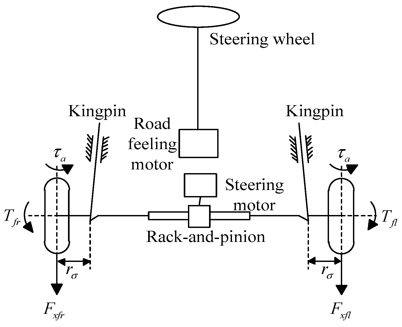
As we all know, when the braking force between the left and right sides is different, the vehicle will turn to the side with larger braking force. Similarly, the different driving force between the left and right sides will drive the steering wheel to generate the steering motion and the vehicle will turn to the side with smaller driving force. Differential steering system of the 4WID EV equipped with an SBW system and the force acting on the vehicle body are shown in Figure 2 and Figure 3, respectively.

The driver’s intention is provided to the electronic control unit (ECU), which gives instructions to the steering mechanism and achieves the steering according to the collected signals and internal control procedures. However, when the SBW system fails suddenly, the steering can only be realized by the differential driving torque, which can also generate the front wheel angles simultaneously.

The dynamic equation of the steering system (shown in Figure 2) can be written as [11]:

$$J_e{\ddot{\delta }}_f+b_e{\dot{\delta }}_f={\tau }_a+\frac{\Delta M}{R}{r}_{\sigma }-{\tau }_f,$$

(8)

$${\tau }_a=k_f{\alpha }_f{l}^2/3,$$

(9)

$${\alpha }_f=\beta +l_f\gamma /u_x-{\delta }_f,$$

(10)

where $J_e$ and $b_e$ are the effective moment of inertia and damping of the SBW system, ${\delta }_f$ is the front wheel steering angle, ${\tau }_a$ is the tire self-aligning moment, $r_{\sigma }$ is the scrub radius, ${\tau }_f$ is the friction torque, ${\alpha }_f$ is the tire slip angle of the front wheel, l is the half of the tire contact length. In addition,${\ddot{\delta }}_f$ and ${\tau }_f$ can be assumed as bounded disturbances.

The lateral and yaw motion (shown in Figure 3) of the EV can be expressed as:

$$\{\begin{array}{l}m{u}_x(\dot{\beta }+\gamma )=\left(F_{yfl}+F_{yfr}\right)\cos {\delta }_f+\left(F_{xfl}+F_{xfr}\right)\sin {\delta }_f+F_{yrl}+F_{yrr}\\ I_Z\dot{\gamma }=\left(l_f\sin {\delta }_f+l_s\cos {\delta }_f\right)\frac{\Delta M}{R}+\left(l_f\cos {\delta }_f-l_s\sin {\delta }_f\right)(F_{yfl}+F_{yfr})-l_r(F_{yrl}+F_{yrr})\end{array},$$

(11)

where

$$F_{yfl}=F_{yfr}=k_f\left(\beta +l_f\gamma /u_x-{\delta }_f\right),F_{yrl}=F_{yrr}=k_r\left(\beta -l_r\gamma /u_x\right).$$

(12)

Define $X\left(t\right)={\left[\begin{array}{ccc}\beta & \gamma & {\delta }_f\end{array}\right]}^T$, $U\left(t\right)=\Delta M$, the state equation can be obtained as

$$\dot{X}=A_{s}X+B_{s}U,$$

(13)

where

$$A_s=\left[\begin{array}{ccc}\frac{2k_f+2k_r}{m{u}_x}& \frac{2k_f{l}_f-2k_r{l}_{\mathrm{r}}}{m{u}_x^2}-1& \frac{2k_f}{m{u}_x}\\ \frac{2k_f{l}_f-2k_r{l}_r}{I_Z}& \frac{2k_f{l}_f^2-2k_r{l}_r^2}{I_Z{u}_x}& -\frac{2k_f{l}_f}{I_Z}\\ \frac{k_f{l}^2}{3b_e}& \frac{k_f{l}^2{l}_f}{3b_e{u}_x}& -\frac{k_f{l}^2}{3b_e}\end{array}\right],B_s=\left[\begin{array}{c}0\\ \frac{l_s}{I_{Z}R}\\ \frac{r_{\sigma }}{R{b}_e}\end{array}\right].$$

(14)

Note: From Equations (1) and (11), it is not difficult to see that they are similar to each other and there are so many ${\delta }_f$ emerged in Equation (11). However, here ${\delta }_f$ is not the external input of the system, but the steering angle of front wheels produced by the differential driving torque between the two sides of the front wheels.

2.3. Reference Model

Here the 2DOF vehicle model with neutral steering characteristics, which can be easily obtained by adjusting the position of the CG, is employed to calculate the reference side-slip angle and yaw rate, and to estimate the actual side-slip angle.

Define x_d(t) = [β_d, γ_d]^T and u_d = $\delta$, the corresponding state equation is expressed as:

$$\{\begin{array}{l}{\dot{x}}_d=A_d{x}_d+B_d{u}_d\\ y_d=C_d{x}_d\end{array}$$

(15)

$$A_d=\left(\begin{array}{cc}\frac{2(k_{f0}+k_{r0})}{m{u}_x}& -1+\frac{2l_{fd}{k}_{f0}-2l_{rd}{k}_{r0}}{m{u}_x^2}\\ \frac{2l_{fd}{k}_{f0}-2l_{rd}{k}_{r0}}{I_Z}& \frac{2l_{fd}{}^2{k}_{f0}+2l_{rd}{}^2{k}_{r0}}{I_z{u}_x}\end{array}\right),B_d=\left(\begin{array}{c}-\frac{2k_{f0}}{m{u}_x}\\ -\frac{2l_{fd}{k}_{f0}}{I_Z}\end{array}\right),C_d=\left(\begin{array}{cc}1& 0\\ 0& 1\end{array}\right).$$

(16)

where β_d and γ_d are the sideslip angle and the yaw rate of the reference model, l_fd and l_rd are the distances from the CG to the front and rear axles, respectively.

2.4. Problem Formulation

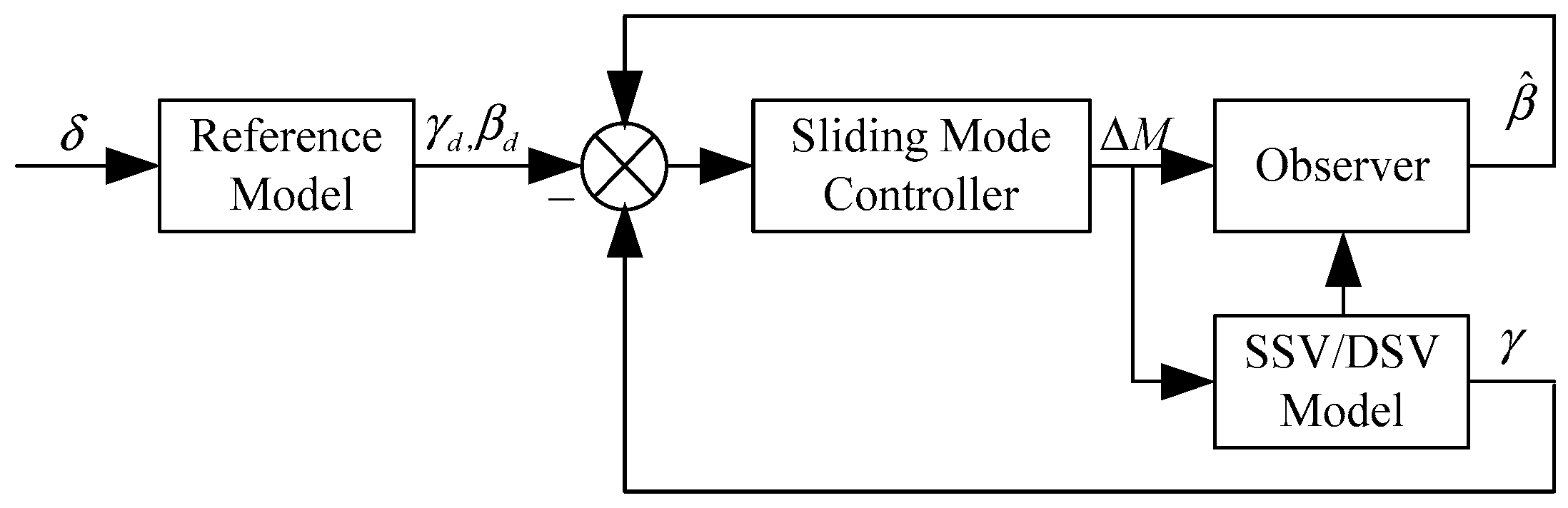
For the reference model, the normal input is the front wheel steering angle, which is proportional to the steering angle commanded by the driver. But for the SSV and DSV in the case of the steering failure, both of their inputs are the differential drive torque between the left and right front wheels, which should be controlled to drive the sideslip angle and yaw rate of the vehicles to their desired ones calculated by Equation (15). The sensors to measure the sideslip angle are usually very expensive. Consequently, the state observer should be firstly designed to estimate the actual sideslip angle. In addition, there is no direct relationship between the steering wheel angle and differential drive torque. To obtain the desired vehicle performance, sliding mode variable structure control strategy is applied. The diagram of control design is depicted in Figure 4.

3. Controllers Design

3.1. Sideslip Angle Observer

The designs of the reduced-order observers for the SSV and the DSV are similar. This subsection takes the DSV as an example to illustrate the method. According to the Equation (13), the following equation can be obtained:

$$\{\begin{array}{l}\left[\begin{array}{l}{\dot{\overline{X}}}_1\\ {\dot{\overline{X}}}_2\end{array}\right]=\left[\begin{array}{cc}{\overline{A}}_{11}& {\overline{A}}_{12}\\ {\overline{A}}_{21}& {\overline{A}}_{22}\end{array}\right]\left[\begin{array}{l}{\overline{X}}_1\\ {\overline{X}}_2\end{array}\right]+\left[\begin{array}{l}{\overline{B}}_1\\ {\overline{B}}_2\end{array}\right]U\\ \overline{Y}=\left[\begin{array}{cc}0& I\end{array}\right]\left[\begin{array}{l}{\overline{X}}_1\\ {\overline{X}}_2\end{array}\right]={\overline{X}}_2\end{array},$$

(17)

where

$$\begin{gathered} {\overline{X}}_1=\left[\beta \right],{\overline{X}}_2=\left[\begin{array}{cc}\gamma & {\delta }_f\end{array}\right],{\overline{A}}_{11}=\left[\frac{2k_f+2k_r}{m{u}_x}\right],{\overline{A}}_{12}=\left[\begin{array}{cc}\frac{2k_f{l}_f-2k_r{l}_{\mathrm{r}}}{m{u}_x^2}-1& \frac{2k_f}{m{u}_x}\end{array}\right], \\ {\overline{A}}_{21}=\left[\begin{array}{cc}\frac{2k_f{l}_f-2k_r{l}_r}{I_Z}& \frac{2k_f{l}_f^2-2k_r{l}_r^2}{I_Z{u}_x}\\ \frac{k_f{l}^2}{3b_e}& \frac{k_f{l}^2{l}_f}{3b_e{u}_x}\end{array}\right],{\overline{A}}_{22}=\left[\begin{array}{c}-\frac{2k_f{l}_f}{I_Z}\\ -\frac{k_f{l}^2}{3b_e}\end{array}\right],{\overline{B}}_1=\left[0\right]. \end{gathered}$$

(18)

Equation (15) can be rewritten as:

$$\{\begin{array}{l}{\dot{\overline{X}}}_1={\overline{A}}_{11}{\overline{X}}_1+v\\ Z={\overline{A}}_{21}{\overline{X}}_1\end{array},$$

(19)

where

$$v={\overline{A}}_{12}\overline{Y}+{\overline{B}}_{1}U, Z=\dot{\overline{Y}}-{\overline{A}}_{22}\overline{Y}-{\overline{B}}_{2}U.$$

(20)

The dynamic equation of the observer is as follows,

$$\{\begin{array}{l}{\dot{\widehat{X}}}_1={\overline{A}}_{11}{\overline{X}}_1+v-H\left(\widehat{Z}-Z\right)\\ Z={\overline{A}}_{21}{\widehat{X}}_1\end{array}.$$

(21)

Substituting the Equation (20) and the second expression of Equation (21) into the first one of Equation (21), the following can be obtained:

$${\dot{\widehat{X}}}_1=\left({\overline{A}}_{11}-H{\overline{A}}_{21}\right){\widehat{X}}_1+\left({\overline{A}}_{12}\overline{Y}+{\overline{B}}_{1}U\right)+H\left(\dot{\overline{Y}}-{\overline{A}}_{22}\overline{Y}-{\overline{B}}_{2}U\right).$$

(22)

where, $\left({\overline{A}}_{11}-H{\overline{A}}_{21}\right)$ is the coefficient matrix of the observer. And the pole of the reduced-order observer is determined by the following characteristic equation.

$$\left|\lambda I-\left({\overline{A}}_{11}-H{\overline{A}}_{21}\right)\right|=0.$$

(23)

Since Equation (22) contains a derivative term $\dot{\overline{Y}}$, it is necessary to obtain the derivative signal of the output, which will affect the uniqueness of the estimated state ${\widehat{X}}_1$. Alternative state variables are allowed to be selected so that the state equation does not contain the derivative signal.

Define

$$W={\widehat{X}}_1-H\overline{Y},$$

(24)

then,

$${\dot{\widehat{X}}}_1=\dot{W}+H\dot{\overline{Y}}=\left({\overline{A}}_{11}-H{\overline{A}}_{21}\right)\left(W+H\overline{Y}\right)+\left({\overline{A}}_{12}\overline{Y}-{\overline{B}}_{1}U\right)+H\dot{\overline{Y}}-H{\overline{A}}_{22}\overline{Y}-H{\overline{B}}_{2}U.$$

(25)

And the following expression can be obtained from

$$\{\begin{array}{l}{\widehat{X}}_1=W+H\overline{Y}\\ \dot{W}=\left({\overline{A}}_{11}-H{\overline{A}}_{21}\right)W+\left({\overline{B}}_1-H{\overline{B}}_2\right)U+\left[\left({\overline{A}}_{11}-H{\overline{A}}_{21}\right)H+{\overline{A}}_{12}-H{\overline{A}}_{22}\right]\overline{Y}\end{array}.$$

(26)

Subtracting Equation (22) from the first expression of Equation (19), and

$${\dot{\overline{X}}}_1-{\dot{\widehat{X}}}_1=\left({\overline{A}}_{11}{\overline{X}}_1+{\overline{A}}_{12}\overline{Y}+{\overline{B}}_{1}U\right)-\left({\overline{A}}_{11}-H{\overline{A}}_{21}\right){\widehat{X}}_1-\left({\overline{A}}_{12}\overline{Y}+{\overline{B}}_{1}U\right)-H\left(\dot{\overline{Y}}-{\overline{A}}_{22}\overline{Y}-{\overline{B}}_{2}U\right),$$

(27)

then it can be simplified as follows

$${\dot{\overline{X}}}_1-{\dot{\widehat{X}}}_1={\overline{A}}_{11}{\overline{X}}_1-\left({\overline{A}}_{11}-H{\overline{A}}_{21}\right){\widehat{X}}_1-H{\overline{A}}_{21}{\overline{X}}_1=({\overline{A}}_{11}-H{\overline{A}}_{21})\left({\overline{X}}_1-{\widehat{X}}_1\right).$$

(28)

This equation is homogeneous. So long as H is properly selected, the poles of the reduced-order observer can be disposed arbitrarily [14], so that the satisfactory attenuation speed of $\left({\overline{X}}_1-{\widehat{X}}_1\right)$ can be obtained and the state estimation ${\widehat{X}}_1$ can approach ${\overline{X}}_1$ as soon as possible.

3.2. Sliding Mode Controller of Skid Steering Vehicle

For the SSV there is no direct relationship between the steering wheel angle and differential drive torque, the traditional vehicle with neutral steering characteristic is used as the reference model. And the SMC controller based on uncertain parameters is designed to make sure that the state variables of skid steering vehicle to track those of the reference model.

Define the state variables of error system as $e=x_d-x$, and the error model is as follows:

$$\dot{e}=A_{d}e+\left(A_d-A_0\right)x+B_d{u}_d-Bu-\Delta Ax.$$

(29)

The nominal model of the error system can be expressed as:

$$\dot{e}=A_{d}e+\left(A_d-A_0\right)x+B_d{u}_d-Bu.$$

(30)

In order to control the output of SSV completely tracking that of the reference model, u should satisfy the following equation for arbitrary state x, external reference input u_d and various uncertainties.

$$\left(A_d-A_0\right)x+B_d{u}_d-Bu-\Delta Ax=0.$$

(31)

According to the linear system theory, it can be drawn that the necessary and sufficient conditions which the controlled object completely tracks the reference model are as follows [15]:

$$rank[B]=rank[\begin{array}{cc}B& \Delta A\end{array}]=rank[\begin{array}{cc}B& C\end{array}],$$

(32)

$$rank[B]=rank[\begin{array}{cc}B& A_d-A\end{array}]=rank[\begin{array}{cc}B& B_d\end{array}].$$

(33)

where Equation (32) is the matching condition as well as Equation (33) is the uncertainty matching condition.

At this point, the controlled system can be rewritten as:

$$\{\begin{array}{l}\dot{x}=A_{0}x+B\left(u+\Delta \tilde{A}x+\Delta \tilde{B}u\right)\\ y=Cx\\ \Delta A=B\Delta \tilde{A},\Delta B=B\Delta \tilde{B}\end{array}$$

(34)

The complete compensation for uncertainties can be achieved by designing the control law. The full-scale sliding mode switching surface for the error model is selected as:

$$s=Ge,$$

(35)

where, $G$ is the sliding mode parameter matrix to be designed and $G=\left[\begin{array}{cc}{G}_1& G_2\end{array}\right]$.

The structure of the variable structure control law can be expressed as:

$$u=u_m+u_v,$$

(36)

where, $u_m$ is the matching control law for the model reference closed-loop control system, $u_v$ is the variable structure control law.

As long as the matrix B is full rank, i.e., rank(B) = m, there must be a non-singular linear transformation matrix T to make ${\tilde{B}}_1=T_{1}B=0$, then the Equation (29) can be transformed into

$$\dot{z}={\tilde{A}}_{d}z+A_{dp}x+{\tilde{B}}_d\delta -\tilde{B}u-\Delta \tilde{A}x,$$

(37)

where

$${\tilde{A}}_d=T{A}_d{T}^{-1},A_{dp}=T\left(A_d-A\right),{\tilde{B}}_d=T{B}_d,\tilde{B}=TB,\Delta \tilde{A}=T\Delta A.$$

(38)

In order to get the appropriate $\tilde{B}$, select

$$T=\left[\begin{array}{cc}{I}_{n-m}& -B_1{B}_2^{-1}\\ 0& I_m\end{array}\right]=\left[\begin{array}{c}{T}_1\\ T_2\end{array}\right].$$

(39)

then

$$z=\left[\begin{array}{c}{z}_1\\ z_2\end{array}\right], {\tilde{A}}_d=T{A}_d{T}^{-1}=\left[\begin{array}{cc}{\tilde{A}}_d^{11}& {\tilde{A}}_d^{12}\\ {\tilde{A}}_d^{21}& {\tilde{A}}_d^{22}\end{array}\right], \tilde{B}=TB=\left[\begin{array}{c}{\tilde{B}}_1\\ {\tilde{B}}_2\end{array}\right]=\left[\begin{array}{c}0\\ {\tilde{B}}_2\end{array}\right],$$

(40)

where $z_1\in R^{n-m}$, $z_2\in R^m$, ${\tilde{A}}_d^{11}\in R^{\left(n-m\right)\times (n-m)}$, ${\tilde{A}}_d^{22}\in R^{m\times m}$, ${\tilde{B}}_2\in R^{m\times m}$.

And the switching surface becomes

$$s=Ge=\tilde{G}Te=\tilde{G}z=\left({\tilde{G}}_1,{\tilde{G}}_2\right)z.$$

(41)

The pole assignment method is used to compute $G$, which makes the final sliding mode have the pre-given pole set $\Lambda =\left\{{\lambda }_i,i=1,2,\dots ,n-m\right\}$ (where all of the poles have negative real parts and imaginary parts appear in pairs). Since $\left({\tilde{A}}_d^{11},{\tilde{A}}_d^{12}\right)$ is a controllable matrix, there is matrix K to ensure that pole set of ${\tilde{A}}_d^{11}-{\tilde{A}}_d^{12}K$ is $\Lambda$.

In addition, since

$$\tilde{G}=\left[{\tilde{G}}_1,{\tilde{G}}_2\right]=\left[{\tilde{G}}_{2}K,{\tilde{G}}_2\right]={\tilde{G}}_2\left[K,I\right],$$

(42)

where ${\tilde{G}}_2$ is a non-singular matrix of m ×m, and usually ${\tilde{G}}_2=I_m$. And $\tilde{G}=\left[K,I\right]$ can be confirmed uniquely, and the switching function $s=Ge$ is obtained.

According to the matching condition of fully matched model, the matching control law is as follows.

$$u_m={\tilde{B}}_2^{-1}\left[\begin{array}{cc}0& I_m\end{array}\right]T(A_d-A)x+{\tilde{B}}_2^{-1}\left[\begin{array}{cc}0& I_m\end{array}\right]B_d\delta .$$

(43)

Substituting Equations (36) and (43) into the Equation (37), the error equation becomes:

$$\dot{z}={\tilde{A}}_{d}z-\tilde{B}{u}_v-\Delta \tilde{A}x,$$

(44)

where the variable structure control law $u_v$ can be chosen to ensure that the system is stable and reliably maintained in the sliding mode, which means that $u_v$ can make the sliding mode reach the condition, $\frac{d}{dt}\left(s^{T}Qs\right)<0$, where $Q$ is the symmetric positive definite matrix and $Q>0$. So $u_v$ should make the following equation hold.

$$\dot{w}=s^T\dot{s}<0.$$

(45)

Let

$$u_v=g\left(t\right){\left(G\tilde{B}\right)}^{-1}\mathrm{sgn}\left(s\right),$$

(46)

where g(t) is the scalar control coefficient to be determined and g(t) > 0, then

$$\dot{w}=s^T\left[C\left(A_0+\Delta A\right)x+CBu\right].$$

(47)

Substituting Equation (46) into Equation (47), then

$$\dot{w}=-g\left(t\right)s^{T}sgn\left(s\right)+s^T\left[G{\tilde{A}}_{m}z-G\Delta \tilde{A}x\right]\le -g\left(t\right)\Vert s^T\Vert +\Vert s^T\Vert \left[\Vert G{\tilde{A}}_m\Vert \Vert z\Vert +{\varphi }_a\Vert G\Vert \Vert x\Vert \right].$$

(48)

And the control law is

$$g\left(t\right)=a_1\Vert z\Vert +a_2\Vert x\Vert +a_3+\epsilon ,a_1=\Vert G{\tilde{A}}_m\Vert ,a_2={\varphi }_a\Vert G\Vert .$$

(49)

where ε is a small positive number. After obtaining the above control law, the variable structure control law of the full-scale sliding mode model can be got by transforming z into e.

3.3. Sliding Mode Controller of Differential Steering Vehicle

Here the sliding surface of SMC can be defined as the following to make sure that the real sideslip angle and yaw rate approach the ideal ones.

$$s=\gamma -{\gamma }_d+\xi \left(\widehat{\beta }-{\beta }_d\right),$$

(50)

where, $\xi$ is the weight coefficient, which is used to enhance or reduce the influence of sideslip angle. Take the derivative of Equation (50) and substitute Equations (11) and (26) into Equation (50), the following equation can be obtained:

$$\dot{s}=d_1+d_2+\frac{l_s}{I_{Z}R}\Delta M+D_1\left(t\right),$$

(51)

where

$$\begin{gathered} d_1=-\frac{2k_f{l}_f}{I_Z}{\delta }_f+\frac{2k_f{l}_f-2k_r{l}_r}{I_Z}\beta +\frac{2k_f{l}_f^2-2k_r{l}_r^2}{I_Z{u}_x}\gamma , \\ {d}_2=\xi \left[\frac{2k_f}{m{u}_x}{\delta }_f+\frac{2k_f+2k_r}{m{u}_x}\beta +\left(\frac{2k_f{l}_f-2k_r{l}_{\mathrm{r}}}{m{u}_x^2}-1\right)\gamma \right], \\ {D}_1\left(t\right)=-\left[{\dot{\gamma }}_d+\xi {\dot{\beta }}_d-\xi ({\overline{A}}_{11}-H{\overline{A}}_{21})\left(\beta -\widehat{\beta }\right)\right]. \end{gathered}$$

(52)

Note that the sideslip angle observer is convergent, that is, the observer error $\beta -\widehat{\beta }$ converges to zero in a finite time. And from the Equation (11), it can be drawn that ${\dot{\gamma }}_d$, ${\dot{\beta }}_d$ is bounded. Then the following inequality holds.

$$\left|D_1\left(t\right)\right|\le {\overline{D}}_1,$$

(53)

where ${\overline{D}}_1$ is a constant.

In order to weaken the chattering phenomenon of sliding mode control, the exponential reaching law with saturation function is applied, and the controller can be designed as

$$\Delta M=\frac{I_{Z}R}{l_s}\left[-k_1\mathrm{sat}\left(s\right)-k_{2}s-d_1-d_2\right],$$

(54)

with $k_1>{\overline{D}}_1$, $k_2>0$, and the sliding variable $s$ will converge to the origin in a finite time.

Substitute Equation (54) into Equation (51), and

$$\dot{s}=\frac{1}{I_Z}\left[-k_1\mathrm{sat}\left(s\right)-k_{2}s+D_1\left(t\right)\right].$$

(55)

Select the Lyapunov function as $V(s)=\frac{1}{2}{s}^2$, take the derivative of $V(s)$ and we get

$$\dot{V}=\frac{1}{I_Z}\left[-k_1\mathrm{sat}\left(s\right)-k_{2}s+D_1\left(t\right)\right]s\le \frac{1}{I_Z}\left(-k_1+{\overline{D}}_1\right)\left|s\right|.$$

(56)

Note $k_1>{\overline{D}}_1$, and we can get

$$\dot{V}<\sqrt{2}\frac{k_1-{\overline{D}}_1}{I_Z}{V}^{\frac{1}{2}}.$$

(57)

According to the finite-time Lyapunov stability theory, the sliding mode variable $s$ will converge to the origin in a finite time.

4. Simulation and Analysis

In this section, Simulink and CarSim are used to confirm the effectiveness of the control systems designed in this paper. The parameters used in the simulation are as follows: m = 1111 kg, I_z = 2031.4 kg m², l_f = 1.04 m, l_r = 1.56 m, l_fd = 1.04 m, l_rd = 1.56 m, l_s = 0.7405 m, R = 0.304 m, k_f0 = −98,202.8 N/rad, k_r0 = −63,947.18 N/rad. The simulation results are explained in the following subsections.

4.1. Simulation in J-Turn Manoeuvre

In this simulation, u_x = 10 m/s and the steering wheel steering angle with a maximum steering angle of 3.5 rad as shown in Figure 5a is used as the input of the reference model. Figure 5b–l illustrate the simulation results of reference model, SSV and DSV with different SMC controllers.

Figure 5b,c are the calculated and the estimated sideslip angles of the SSV and the DSV with SMC controller. It can be drawn that the designed sideslip angle observer is effective to track the calculated sideslip angle. Figure 5d,e are the yaw rate and sideslip angle curves of the three models. It can be seen that both of the yaw rate and sideslip angle of DSV with SMC controller can follow the desired ones, while only the yaw rate of SSV with SMC controller can follow the desired one. Generally speaking, the side slip angle and the yaw rate are coupled. It is often difficult to track two state variables simultaneously by a single control variable—differential torque. Here the desired yaw rate is tracked very well.

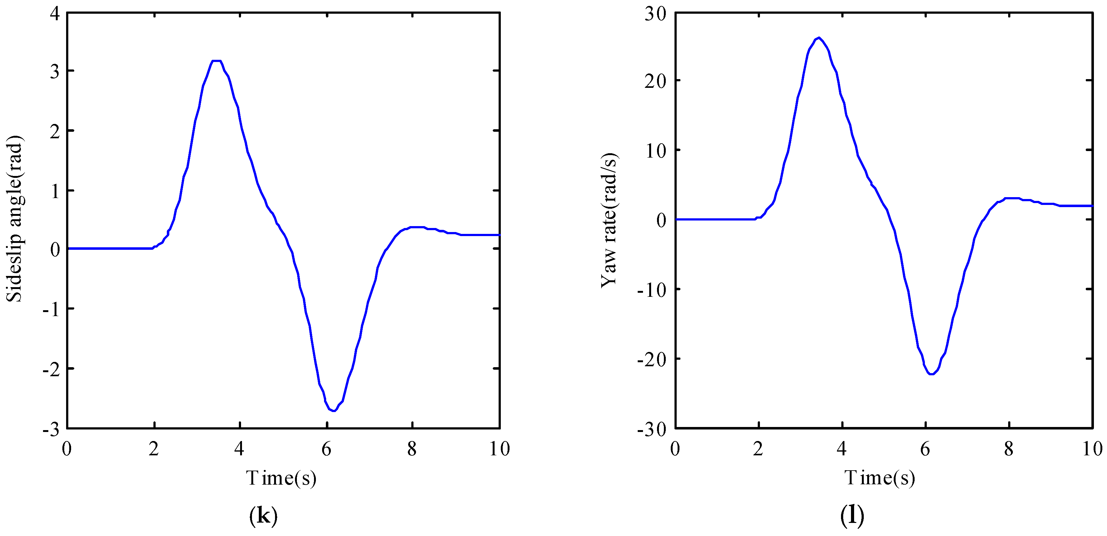
Figure 5f,g show that the differential driving torques for the controllers of SSV and DSV respectively, and their absolute maximum are 142,210 Nm and 75.86 Nm. Obviously, there is too large a difference between the two needed differential driving torques. The reason is for the DSV the differential torque also produces a front wheel steering angle at the same time, which decreases the needed differential torque in turn. And the maximum front wheel angle produced by the differential driving torque for the controller of DSV are 0.1745 rad as shown in Figure 5h. Figure 5i–l are the response curves of SSV and DSV without SMC controller. It can be seen that they are so different from the desired ones.

In conclusion, the simulation results show that the designed observer is effective and the responses of DSV with SMC controller can exactly track the ideal ones. Although the yaw rate of SSV with SMC controller can also exactly track that of the reference model, the differential driving torque needed for SSV is too much larger than that needed for DSV, which obviously exceeds the maximum torque provided by the in-wheel motor.

4.2. Simulation in Double Lane Change Maneuver

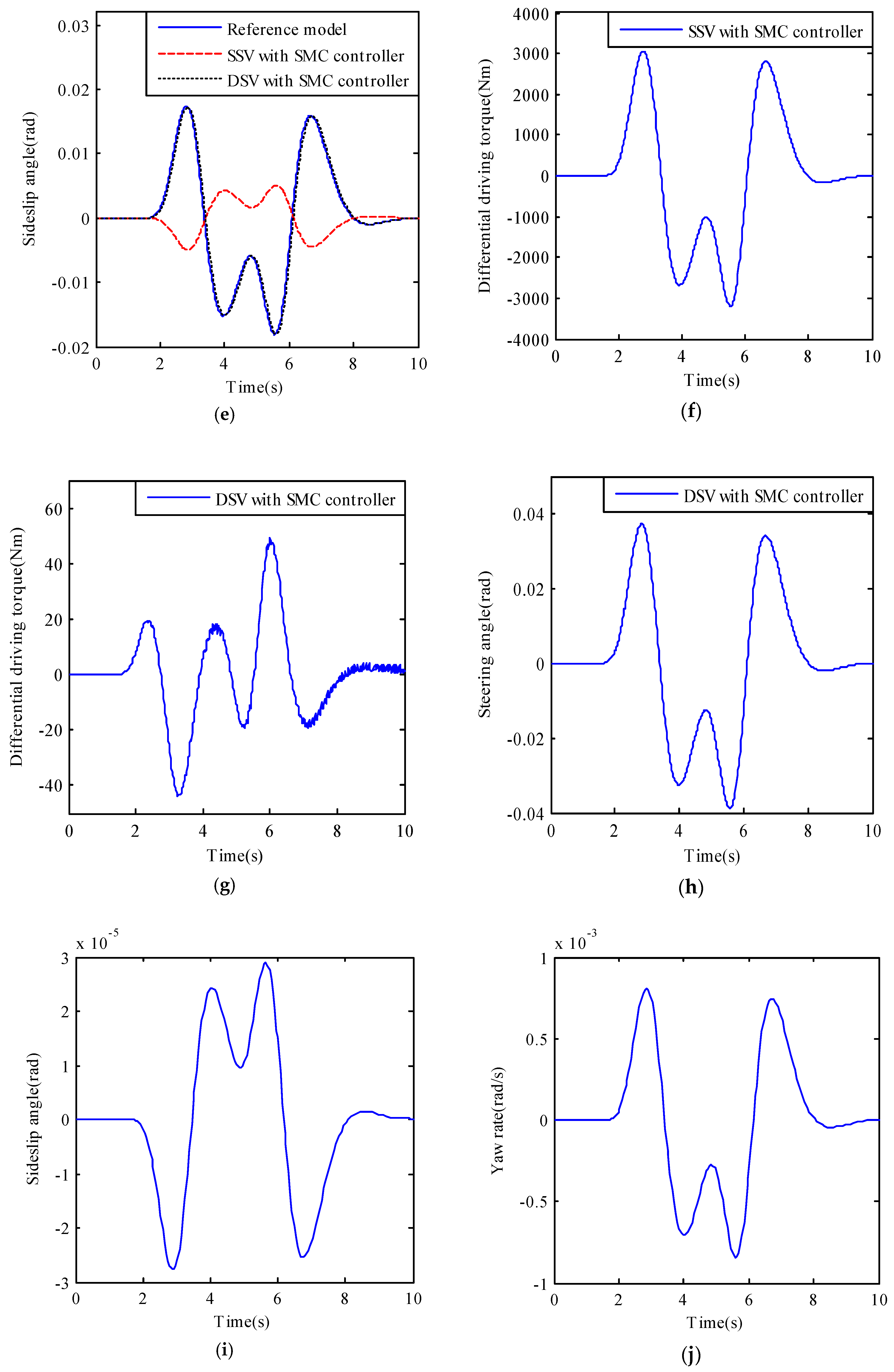
Double lane change maneuver is another important method to examine the maneuvering stability of the vehicle. In this simulation, u_x = 20 m/s and Figure 6a shows the input of the reference model, which can guarantee the vehicle to achieve the double lane change maneuver. Figure 6b–l illustrate the simulation results of reference model, SSV and DSV with different SMC controllers.

Figure 6b,c are the calculated and the estimated sideslip angles of the SSV and the DSV with SMC controller, which show that the designed observer can track the calculated sideslip angle very well. Figure 6d is the yaw rate curves of the three models and their responses are almost the same. Figure 6e is the sideslip angles of the three models, which illustrates that only the sideslip angle of the SSV with controller can follow the desired one. The differential drive torques between the left and right front wheels required for the SSV and the DSV with SMC controller are shown in Figure 6f,g and their absolute maximums are 3150 Nm and 46.4 Nm. In addition, the external steering angle of the front wheel is as shown in Figure 6h. Figure 6i–l are the response curves of the SSV and the DSV without SMC controller. It can be seen that they are so different from the desired ones.

In conclusion, both of the differential driving torque and the external steering angle of the front wheel produced by the torque contribute to the steering of DSV with SMC controllers, which leads to a substantial reduction in the required differential driving torque. Therefore, the differential driving torque needed for the DSV is much smaller than that needed for the SSV.

4.3. Robustness Analysis

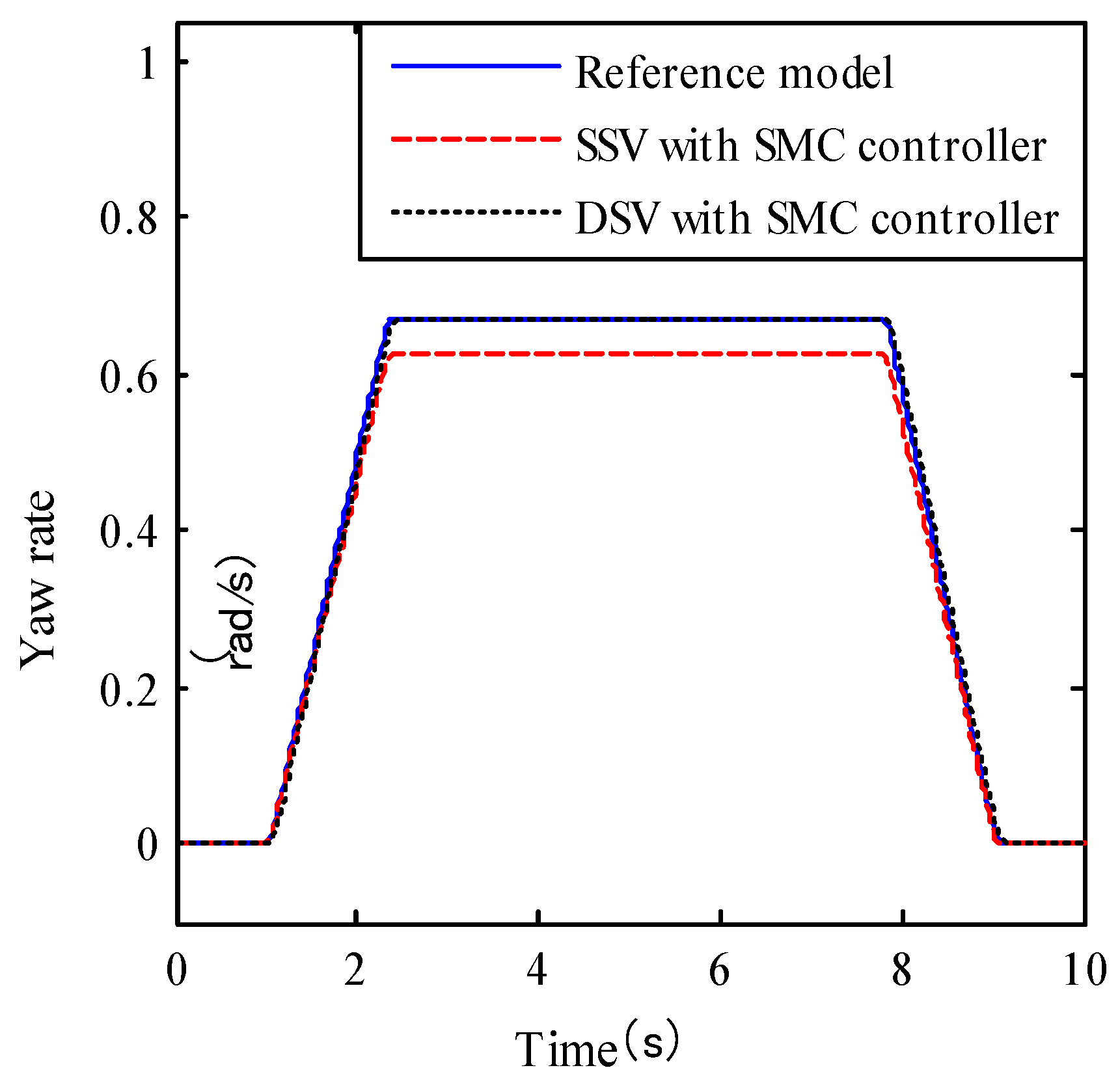
When the cornering stiffness of the front and rear tires are decreased and increased by 5% respectively as other parameters remain unchanged, yaw rate curves of reference model, SSV and DSV with different SMC controllers are shown in Figure 7 and Figure 8, respectively.

From Figure 7 and Figure 8, it can be seen that the yaw rate curve of DSV with SMC controller can completely track that of the reference model when front or rear tire cornering stiffness is changed. However, there are always a little difference between the yaw rates of SSV with SMC controller and the reference model. It can be drawn that the robustness of DSV with SMC controller is better than that of SSV with SMC controller.

5. Conclusions

The realizations of skid steering and differential steering of IWM EVs with the failure of SBW system are studied:

(1)

Simulation results show that the skid steering of SSV can be realized by the differential drive torque between the two sides of the front wheels. However, the needed differential drive torque is so large and far beyond the maximum torque generated by the in-wheel motor. Therefore, the skid steering cannot be used in practice.

(2)

The differential steering of DSV in case of steering failure also can be achieved by the differential drive torque between the two sides of the front wheels. Because this torque generates an external vehicle yaw moment and at the same time an additional steering angle of the front wheel is also produced, so its value can be greatly reduced.

(3)

The structure of differential steering is relatively simple. It not only can be used as the backup steering system, but also can be used for the active steering of front and rear wheels and the improvement of vehicle handling stability, and even can be applied as a sole steering system for future pilotless vehicles.

References

- Leng, B.; Xiong, L.; Jin, C.; Liu, J.; Zhuo, P.Y. Differential Drive Assisted Steering Control for an In-wheel Motor Electric Vehicle. SAE Int. J. Passeng. Cars Electron. Electr. Syst. 2015, 8, 433–441. [Google Scholar] [CrossRef]
- Sun, C.Y.; Zhang, X.; Xi, L.H.; Tian, Y. Design of a path-tracking steering controller for autonomous vehicles. Energies 2018, 11, 1451. [Google Scholar] [CrossRef]
- To, C.N.; Hormoz; Dai, V.Q.; Simic, M.; Khayyam, H.; Marzbani; Jazar, R.N. Autodriver autonomous vehicles control strategy. Procedia Comput. Sci. 2018, 126, 870–877. [Google Scholar] [CrossRef]
- Zhao, W.Z.; Xu, X.H.; Wang, C.Y. Multidiscipline collaborative optimization of differential steering system of electric vehicle with motorized wheels. Sci. China-Technol. Sci. 2012, 55, 3462–3468. [Google Scholar] [CrossRef]
- Li, W.; Potter, T.; Jones, R.P. Steering of 4WD vehicles with independent wheel torque control. Veh. Syst. Dyn. 1998, 29, 205–218. [Google Scholar] [CrossRef]
- Shuang, G.; Cheung, N.C.; Cheng, K.W.E.; Dong, L.; Liao, X. Skid Steering in 4-Wheel-Drive Electric Vehicle. In Proceedings of the 7th International Conference on Power Electronics and Drive Systems, Bangkok, Thailand, 27–30 November 2007; pp. 1548–1553. [Google Scholar]
- Wang, J.; Wang, Q.; Jin, L.; Song, C. Independent wheel torque control of 4WD electric vehicle for differential drive assisted steering. Mechatronics 2011, 21, 63–76. [Google Scholar] [CrossRef]
- Zhao, W.Z.; Li, Y.J.; Wang, C.Y.; Zhang, Z.Q.; Xu, C.L. Research on control strategy for differential steering system based on H mixed sensitivity. Int. J. Automot. Technol. 2013, 14, 913–919. [Google Scholar] [CrossRef]
- Wu, X.D.; Yang, L.; Xu, M. Speed Following Control for Differential Steering of 4WID Electric Vehicle. In Proceedings of the 40th Annual Conference of the IEEE-Industrial-Electronics-Society, Dallas, TX, USA, 29 October–1 November 2014; pp. 3054–3059. [Google Scholar]
- Zhai, L.; Hou, R.F.; Sun, T.M.; Steven, K. Continuous Steering Stability Control Based onan Energy-Saving Torque Distribution Algorithm for a Four in-Wheel-Motor Independent-Drive Electric Vehicle. Energies 2018, 11, 350. [Google Scholar] [CrossRef]
- Wang, R.R.; Jing, H.; Hu, C.; Chadli, M.; Yan, F.J. Robust H∞ output-feedback yaw control for in-wheel motor driven electric vehicles with differential steering. Neurocomputing 2016, 173, 676–684. [Google Scholar] [CrossRef]
- Hu, C.; Wang, R.R.; Yan, F.J.; Karimi, H.R. Robust Composite Nonlinear Feedback Path Following Control for Independently Actuated Autonomous Vehicles with Differential Steering. IEEE Trans. Transp. Electrif. 2016, 2, 1–10. [Google Scholar] [CrossRef]
- Hu, C.; Wang, R.R.; Yan, F.J.; Huang, Y.J.; Wang, H.; Wei, C.F. Differential Steering Based Yaw Stabilization Using ISMC for Independently Actuated Electric Vehicles. In Proceedings of the Symposium of Mechatronic and Embedded Technologies in Intelligent Transporation Systems at the 12th IEEE/ASME International Conference on Mechatronic and Embedded Systems and Applications, Auckland, New Zealand, 29–31 August 2016; Volume19, pp. 627–638. [Google Scholar]
- Xie, H.W.; Zou, F.X.; Zhang, M.; Li, P.B.; Li, Q. Morden Control Systems, 8th ed.; Higher Education Press: Beijing, China, 2006; pp. 201–204. ISBN 7-04-009643-9. [Google Scholar]
- Li, Y.J.; Zhang, K. Theory and Application of Adaptive Control; Northwestern Polytechnical University Press: Xi’an, China, 2005; pp. 168–170. ISBN 7-5612-1875-3. [Google Scholar]