Integrated Photovoltaic Inverters Based on Unified Power Quality Conditioner with Voltage Compensation for Submarine Distribution System


School of Electrical Engineering, Chungbuk National University, Cheongju 28644, Korea
*
Author to whom correspondence should be addressed.
Energies 2018, 11(11), 2927; https://doi.org/10.3390/en11112927
Submission received: 20 September 2018
/
Revised: 20 October 2018
/
Accepted: 23 October 2018
/
Published: 26 October 2018
(This article belongs to the Special Issue Power Quality in Microgrids Based on Distributed Generators)
Abstract
:This paper proposes a multi-functional Photovoltaic (PV) inverter based on the Unified Power Quality Conditioner (UPQC) configuration. Power quality improvement is a difficult issue to solve for isolated areas or islands connected to the mainland through long submarine cables. In the proposed system, the line voltage is compensated for by the series inverter while the shunt inverter delivers the PV generating power to the grid. Depending on the technical conditions of power quality and system environment, it has five different operating modes. Especially during poor power quality conditions, the sensitive load is separated from the normal load to provide a different power quality level by using the microgrid conception. In this paper, the control method and the power flow for each mode are described, and the operational performance is verified through a PSiM simulation so that it can be applied to the power quality improvement of weak grid power systems such as in isolated areas or on islands connected to the mainland by long submarine cables.
1. Introduction
Recently, renewable energy has spread rapidly due to concerns over climate change and environmental issues. The penetration of renewable energy in distribution systems has grown fast to catch up with population growth and reduce the use of conventional energy sources like coal power plants. Distributed generation (DG), such as photovoltaic (PV) systems or windtrubine generation systems, plays a major role in evolving a microgrid. PV energy has been developing for more than 160 years and its growth has increased exponentially in the last two decades. The total installed capacity at the end of 2016 amounted to 303 GW globally [1].
Since the PV system is designed to have significant penetration to the distribution line or submarine cable, the power flow can be reserved and the distribution system is no longer a passive circuit but an active one that can determine the power flow based on the distributed generation as well as the load. The low energy density and long-distance distribution system can make the grid system weak or its short circuit ratio (SCR) low [2,3].
People who live in isolated areas need electricity to manage their daily life. An islands’ power system is usually connected to the mainland through a submarine cable system. However, the undervoltage or overvoltage problems can occur frequently due to the load capacity [4]. As in IEEE 1159, undervoltage is defined as a typical voltage magnitude less than 0.9 pu for a duration longer than 1 min, and overvoltage is defined as a typical voltage magnitude higher than 1.1 pu for a duration longer than 1 min [5]. In normal or heavy load conditions, undervoltage will occur due to cable resistance or cable inductance. On the other hand, in light loads, overvoltage can occur due to submarine cable capacitance—the so-called Ferranti effect [6,7]. In this condition, sensitive electric equipment can be damaged due to undervoltage or overvoltage grid conditions. In real measurements undertaken at Pramuka Island in Indonesia, the undervoltage was so serious that the line voltage decreased by up to 20% in the evening, but the overvoltage caused by the base load was not serious.
At the load side, some loads or equipment are sensitive to power quality problems. These sensitive loads can be differentiated from normal loads by a switch, so the microgrid technology allows each load group to be supplied power at different power quality levels [8]. To supply the electricity to sensitive loads with high power quality, additional power quality solutions (PQS), such as the active power filter or dynamic Uninterruptible Power Supply (UPS), can be installed for sensitive loads [9,10,11]. It is easy to apply all kinds of existing PQS at any location of grid to improve the power quality, but it requires a space for PQS and is a little bit more costly. As an alternative solution, it is possible to add a function of improving power quality to the power inverter of a microgrid [12]. The power inverter in the microgrid system is generally used for the conversion of the DC generating power to AC, so the main function of the inverter is to supply the converted power to the main grid under the output current control. However, the control of the inverter or the topology of the inverter itself can be modified to cover the additional function for the compensation of harmonics or voltage.
In recent years, the development of voltage compensation has led to the implementation of a Dynamic Voltage Restorer (DVR) [13,14,15]. The concept of using DVR for voltage mitigation has had positive results and has achieved popularity since its first use. The DVR with rechargeable energy was suggested to meet the power requirements for voltage disturbance mitigation [13,14], but the authors do not consider the penetration of renewable energy as a source of DVR. Several DVR strategies based on control strategies have also been developed in [15], but the authors do not consider the maximum voltage, which can be compensated for by DVR and the type of the load based on the voltage sensitivity.
The proposed PV inverter system in this research has the voltage compensation function, while the PV power is delivered to the grid. The configuration of the inverter is similar to that of the Unified Power Quality Conditioner (UPQC) [16,17]. It has the topology of the back-to-back inverter, in which one output is connected to the grid in a shunt and the other is connected to the grid in series. To improve the limited function of the conventional DVR in [13,14], the integrated PV system can supply energy to both the DVR and the grid. Therefore, instead of compensating for the harmonics or reactive power in the UPQC, the generated PV power is delivered to the grid through the shunt inverter while the series inverter compensates for the voltage when undervoltage or overvoltage is occurred in the grid [18,19].
To improve the power quality at the system level, all loads are divided into normal loads and sensitive loads groups by integrating the microgrid concept to maintain the power quality at different levels [20]. The voltage compensation operation should be performed only for the sensitive loads group. Depending on the state of the grid voltage, the voltage is compensated for under the grid-connected mode or the regulated voltage is generated under the stand-alone mode without connection to the grid [21]. Therefore, if the grid voltage is in the normal range, the shunt inverter operates only in the PV generation mode. If the grid voltage is outside of the normal range, the grid voltage for only sensitive load is compensated for by the series inverter while the generated PV power is delivered to the grid through the shunt inverter. On the other hand, if the grid voltage deviates from the voltage compensation range, the sensitive loads group is disconnected from the grid and is supplied the power from the PV systems through the shunt inverter. In this mode, it is not necessary to compensate for the voltage through the series inverter, and the normal loads group received power from the grid continuously although the power quality was very poor.
The topology and operation of the PV inverter, which has the additional function of voltage compensation, depending on the state of grid voltage, are described in this paper. The operation mode is defined as a normal mode, a voltage compensation mode, and the stand-alone mode when the grid voltage is in the range of ±10%, ±10 to ±20%, or over ±20%, respectively. During the low irradiance condition, the Battery Energy Storage System (BESS) [22,23] can be a power source in place of the PV source. However, the operation of BESS is applied only for the voltage compensation mode or the stand-alone mode considering the capacity of the batteries. In the voltage compensation mode, the voltage compensation is performed through the series inverter. On the other hand, in stand-alone mode, the shunt inverter supplies the power to the grid without voltage compensation through the series inverter. To analyze the performance of the proposed voltage compensation method, a simulation based on PSIM is conducted.
In this paper, the modeling and problems caused by the submarine cable are described in Section 2. The topology of the proposed PV system with series and shunt inverter is shown in Section 3. In Section 4, the control algorithm and the power flow in every case are explained. Finally, the simulation results and analyses are reported in Section 5, with conclusions in Section 6.
2. Modeling and Analysis of Submarine Cable
2.1. Modeling of Submarine Cable
A submarine cable is installed under the sea to supply power to an isolated island from the mainland or connect an offshore wind turbine system to the main grid. Since it is located near the ground level and has thick insulation, a submarine cable has better capacitive characteristics than an overhead line. Based on a theoretical parallel plate capacitor, the capacitance is inversely proportional to the gap between plates, which corresponds to the distance from the earth in this case. Other factors, such as the distance to other cables (relatively short compared to the overhead line) and the capacitance between conductor and insulation cable, make the submarine cable have better capacitive characteristics than an overhead line.
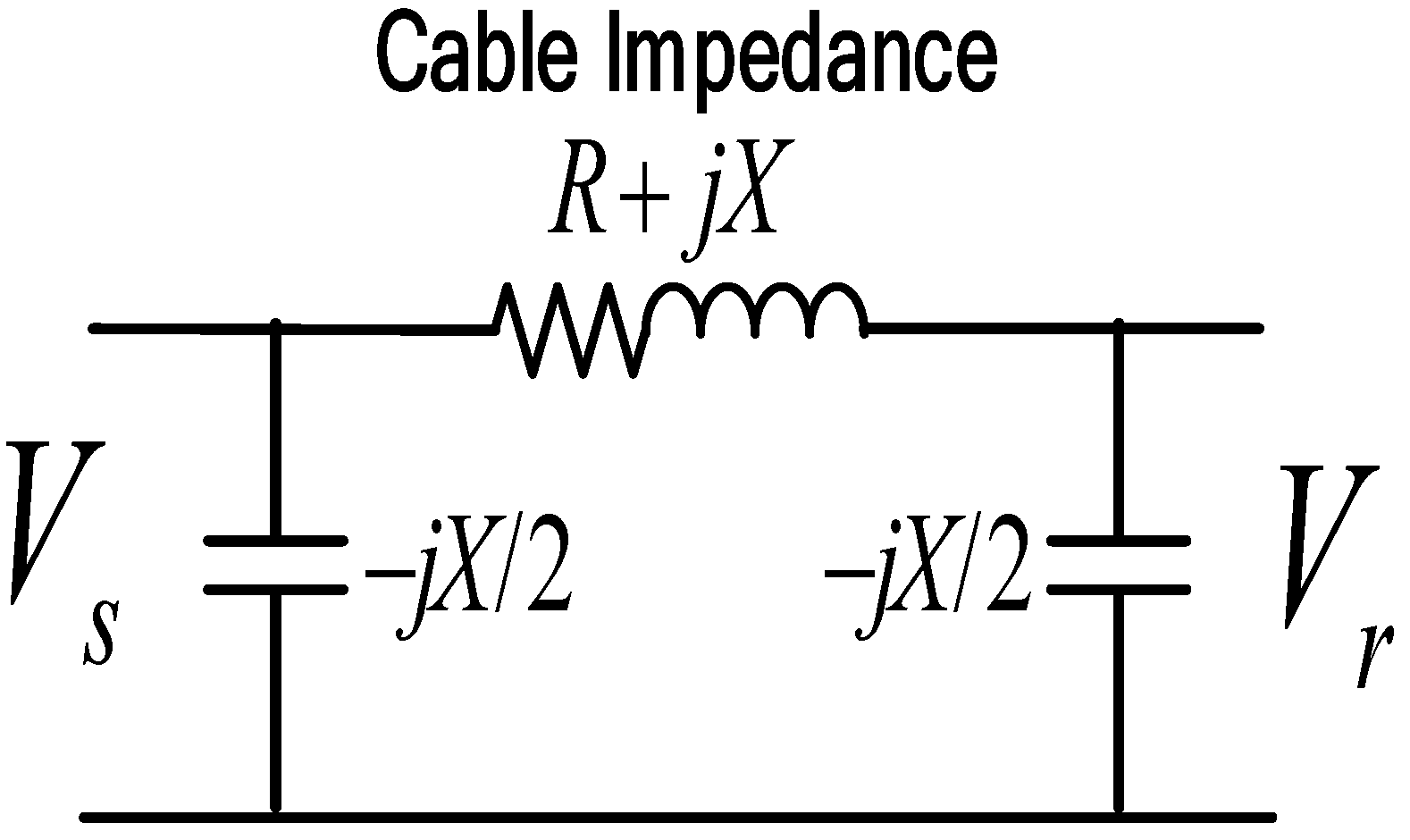
As with the transmission line, the submarine cable can be represented sufficiently well by the resistance (R), inductance (L), and capacitance (C). The difference between the transmission line and the submarine cable is in the short length. The transmission line assumed the shunt admittance of the line is small and can be neglected, but in the submarine cable, the shunt admittance is relatively high and can have an impact on the calculation, as shown in Figure 1. Therefore, in a short submarine cable, the shunt admittance is included in the calculation.
For short and medium lengths, lumped parameters are used, which give better accuracy. However, for the exact solution of any lines longer than 240 km, it should be considered that the parameters of the line are not lumped but distributed uniformly in the line [24].
2.2. Voltage Profile of Submarine Cable
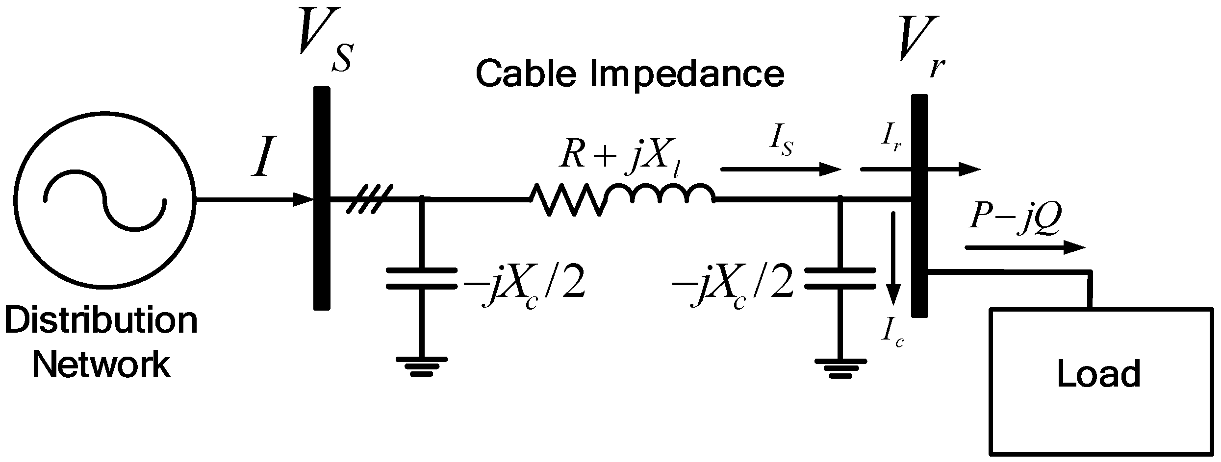
Most of the submarine systems for loads on isolated islands are radial configuration, which gives high impedances. These high impedances lead to the voltage drop or Ferranti effect along the cable from the sending end to the receiving end load. The voltage drop can be calculated from the basic analysis of a two-bus distribution system, as in Figure 2 and Figure 3.
The relationship between the sending end bus voltage, Vs, and the receiving end bus voltage, Vr, is given as in Equation (1):
Substituting Ir and Ic, described as in Equation (2), into Equation (1), we get Equation (3):
If the phase difference between Vs and Vr is neglected based on Vs, then the voltage difference between Vs and Vr can be described as in Equation (4):
This shows that the bus voltage can increase or decrease depending on the amount of active and reactive power consumed at the load and supplied from the Distributed Generator (DG). Based on Equation (4), two conditions can result depending on the load capacity. The voltage difference in Equation (4) can be categorized into two parts: The first part is , and the second part is . In the heavy load condition, the first part is dominant, and the voltage difference, ΔVr, is positive, which means that there is a voltage drop at the receiving end. On the other hand, in light or no-load conditions, the second part is dominant, and the voltage difference, ΔVr, is negative, which means that there is a voltage rise at the receiving end [25]. This is the so-called “Ferranti Effect”.
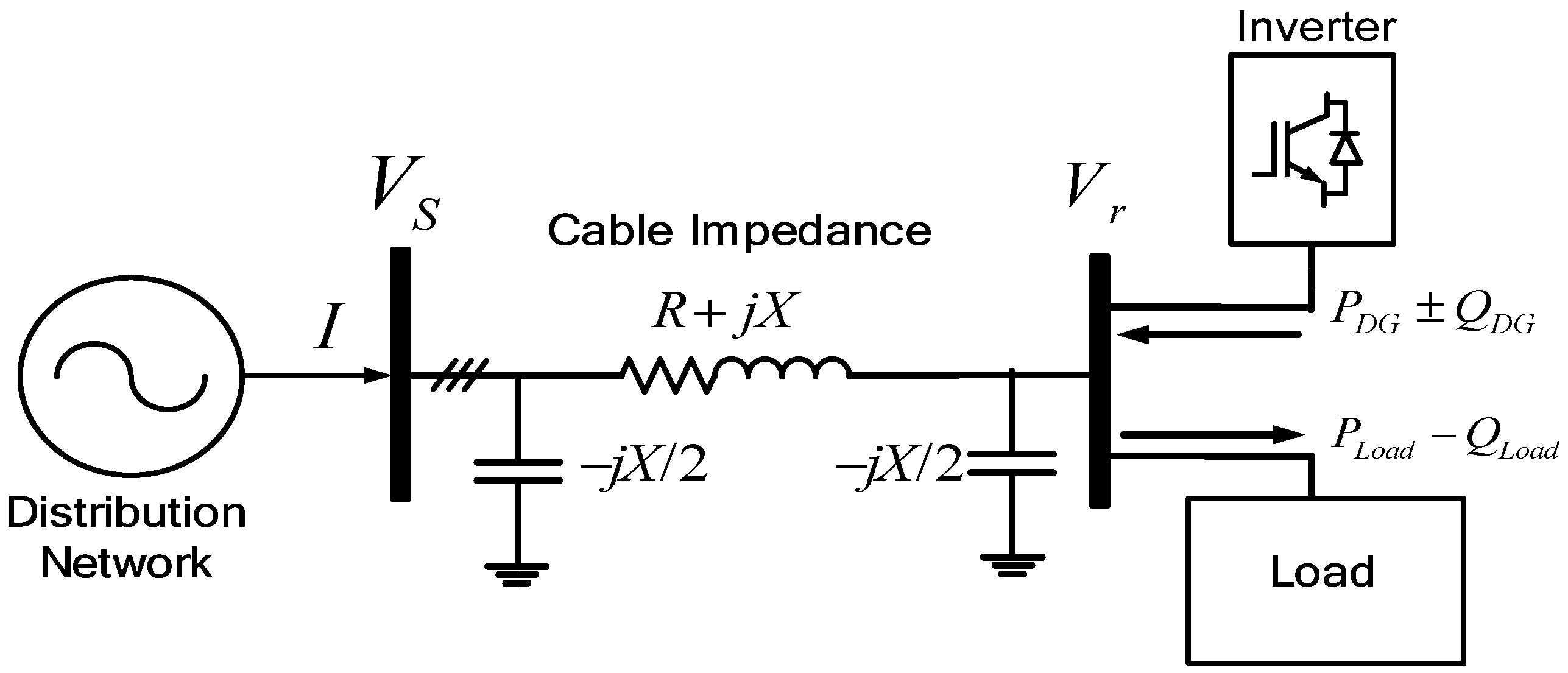
The PV penetration in the distribution system can increase the voltage in the Point of Common Coupling (PCC) bus depending on the power injected by the PV system. Figure 3 shows how the DG can change the voltage at the receiving end since the DG and the power electronics technology can control the active and reactive power injection. In this case, Equation (4) can be modified as in Equation (5):
3. Configuration and Operation of Proposed PV Inverter with Voltage Compensation
3.1. Proposed PV Inverter
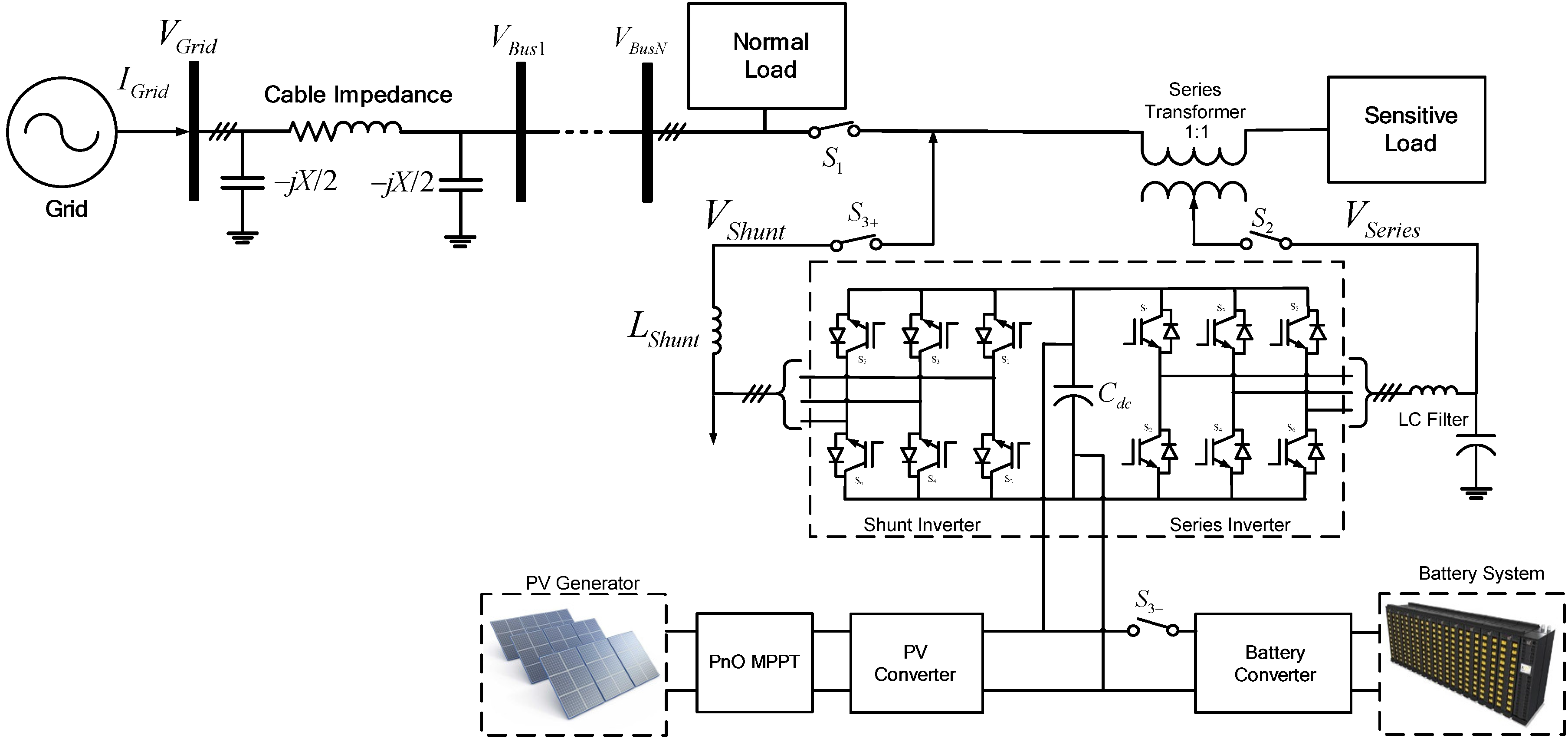
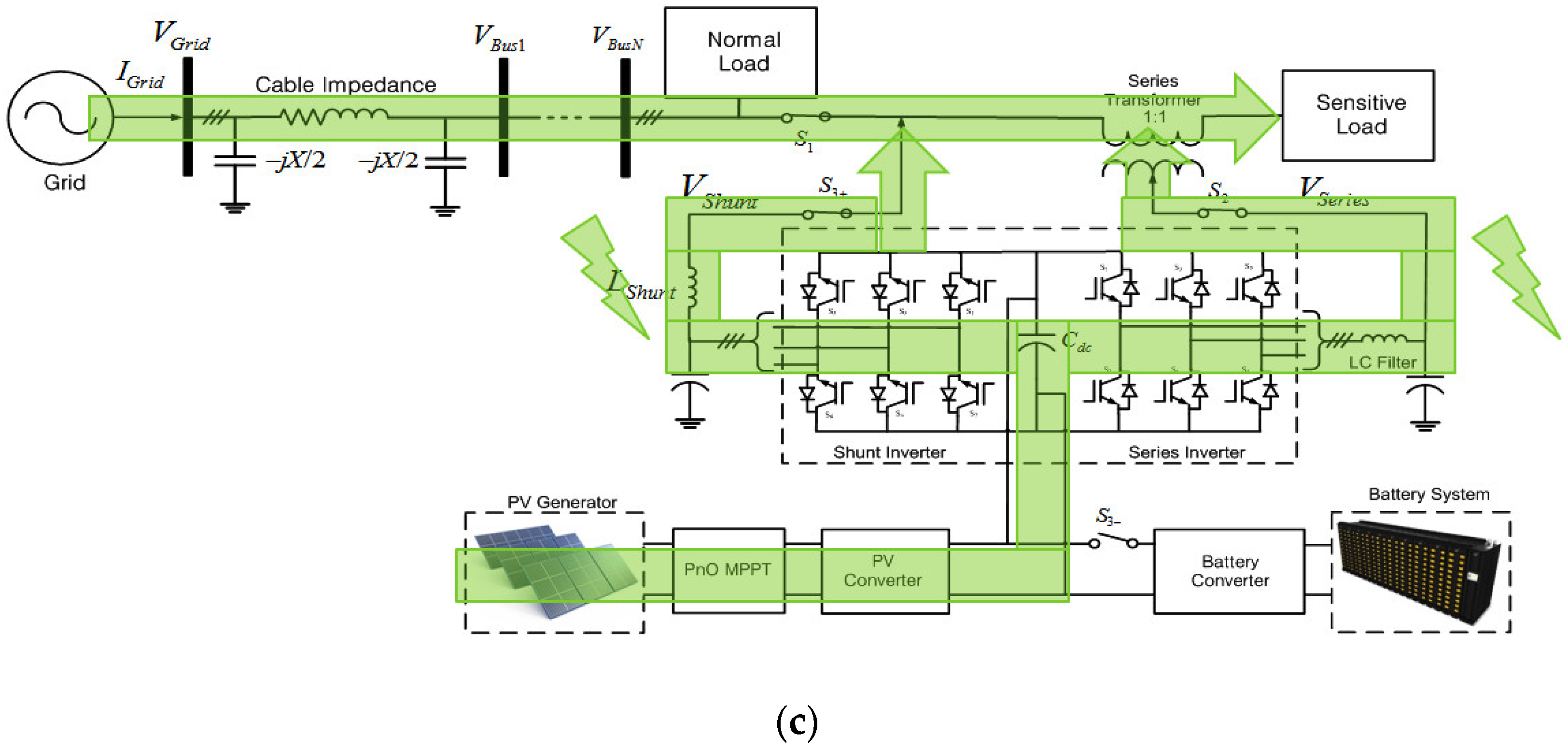
The conventional PV system delivers the power to the grid directly in the grid-connected mode or supplies the power to the load in stand-alone mode without any ability to improve the power quality. However, the proposed system, which has the back-to-back inverter topology of shunt and series inverters based on UPQC configuration, has the additional function of voltage compensation to the conventional PV system, as shown in Figure 4. The sensitive load can be separated from the normal load by disconnecting the switch, and it can be supported at a different power quality level from the normal load by the voltage compensation of the series inverter.
3.2. Operation of Series Inverter
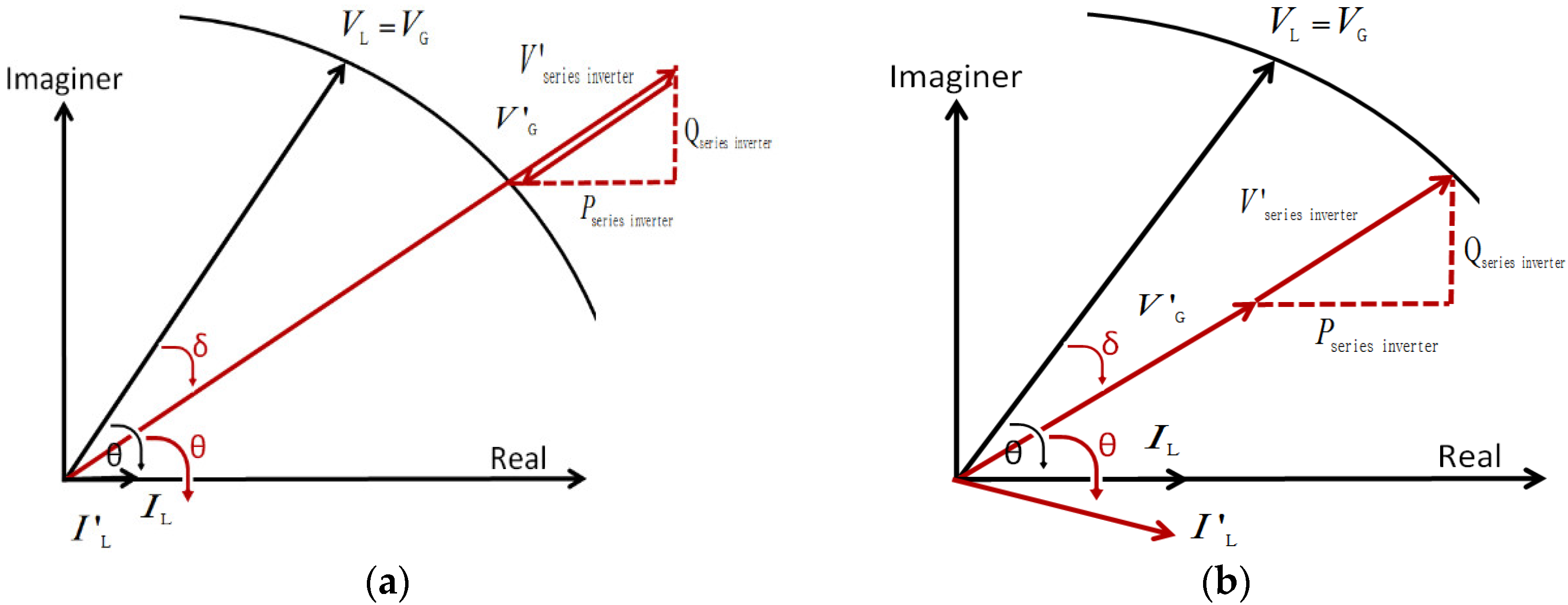
The series inverter is used to compensate for the voltage in the sensitive load in a weak grid system [26,27,28,29,30]. During the light load condition, as shown in Figure 5a, overvoltage, V’G, is occurred, and then the series inverter injected the negative voltage, V’series inverter, into the grid to mitigate it. On the other hand, during heavy load conditions, as shown in Figure 5b, undervoltage, V’G, occurs, so the series inverter injects the positive voltage, V’series inverter, into the grid to mitigate it.
After applying the in-phase voltage compensation method, which makes the series inverter voltage synchronized to the grid voltage, an exchange of active and reactive power between the series inverter and the grid occurs [31]. The voltage and power calculation for series inverter in-phase control scheme is as follows:
3.3. Operation of Shunt Inverter
In this proposed method, the operation of the shunt inverter can be divided into four functions. Firstly, in normal voltage conditions, the shunt inverter injects the maximum power generated from the PV by the Maximum Power Point Tracking (MPPT) method to the grid. Secondly, in undervoltage or overvoltage conditions, the maximum power injected to the grid depends on the power exchanged through the series inverter. In undervoltage conditions, the maximum power injected by the shunt inverter is reduced due to the power necessary for the voltage compensation through the series inverter. On the other hand, in overvoltage conditions, the series inverter absorbs the power from the grid, so the maximum power injected to the grid through the shunt inverter is increased due to the power absorbed from the grid through the series inverter. Thirdly, if the grid voltage is outside the range of voltage compensation or the battery back operation is necessary due the low irradiance, the sensitive load is isolated from the grid by disconnecting the switch. Then, the shunt inverter fully covers the sensitive load in stand-alone mode while the grid supplies power to the normal load even if the power quality is poor. Finally, if the State of Charge (SoC) of BESS is lower than the lower limit during low irradiance conditions, the shunt inverter absorbs power from the grid side and delivers it to the series inverter for voltage compensation. In this mode, the load will be increased due to the power received through the shunt inverter, and this load increase may make the voltage drop in the grid worse. The delivered power through the shunt inverter is described as follows:
4. System Operation Mode and Control of Proposed PV Inverter
There are five operation modes in the proposed PV inverter system, depending on the irradiance condition and the grid voltage magnitude: the normal mode, the voltage compensation mode with PV power, the stand-alone mode, the voltage compensation mode with battery energy, and the voltage compensation mode with the grid power.
4.1. Normal Mode
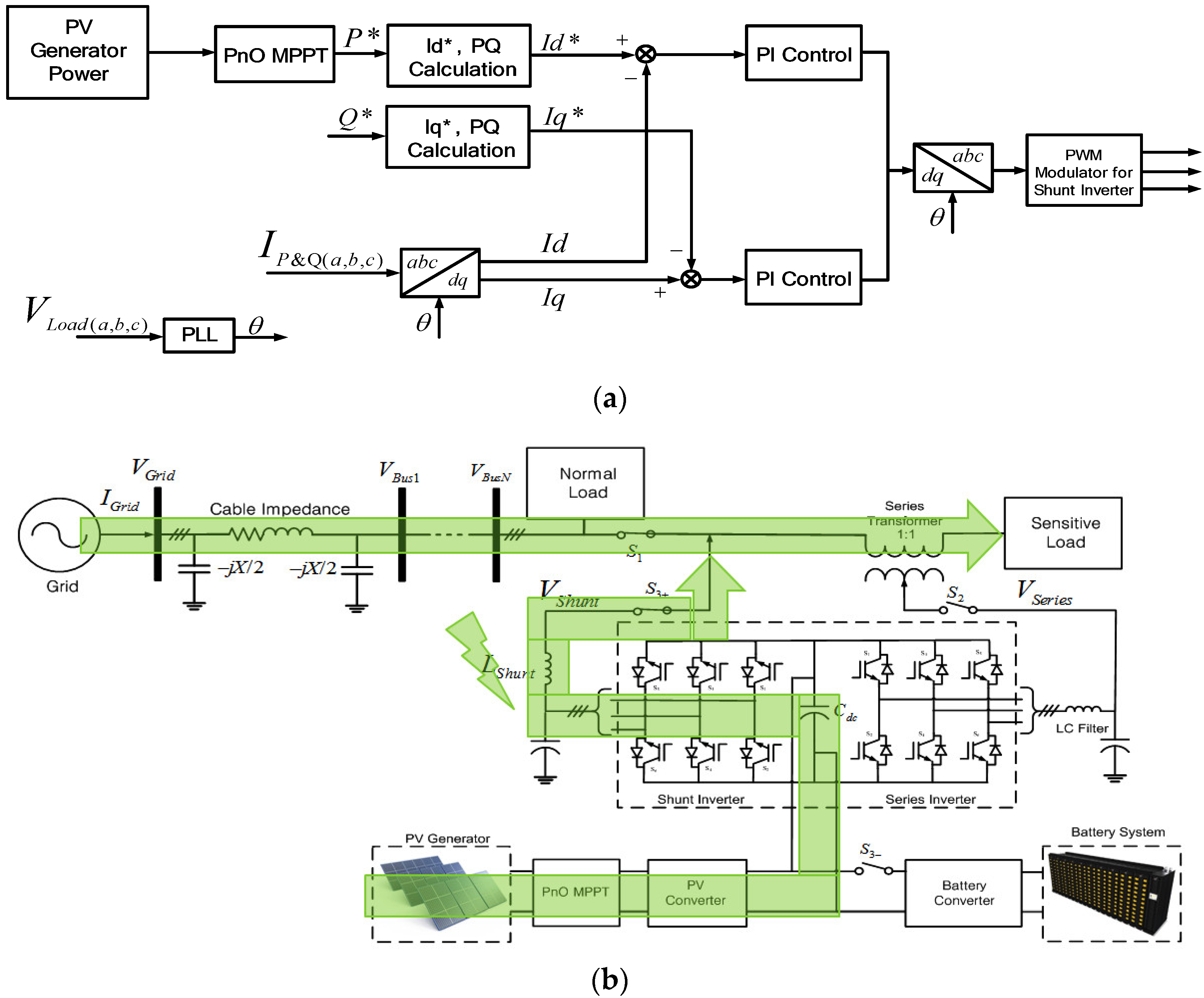
When the grid voltage is under the ±10% range of the rated value, the PV inverter is in the normal mode. In the normal mode, the shunt inverter delivers power to the grid based on the MPPT scheme without any voltage compensation, but the series inverter does not work in this mode. The control scheme for the shunt inverter is shown in Figure 6a. The maximum active power is set to be a reference value of the active power for the PQ control. On the other hand, the reference reactive power is set to be zero to meet the unity power factor operation. The reference values for the active and reactive powers are converted to the reference values of Id and Iq by Equations (11) and (12). Hereinafter, the reference values, I*d and I*q, are subtracted from the real values, Id and Iq, and the PI control is applied to regulate Id and Iq to follow the reference values, I*d and I*q. Finally, the reference dq-frame signal is be transformed to abc domain for Pulse Width Modulation (PWM) generation. The power flow during this mode is shown in Figure 6b.
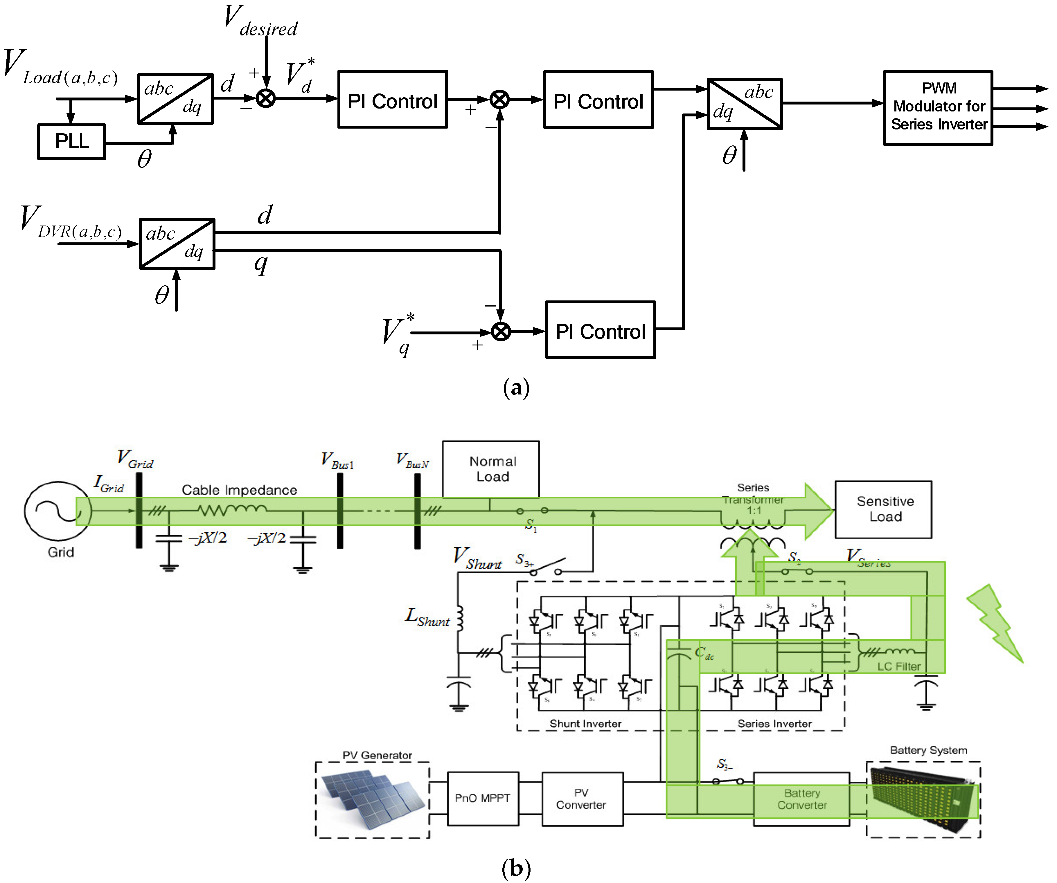
4.2. Voltage Compensation Mode with PV Power
When the grid voltage is between ±10% and ±20% of the rated voltage, it is in the voltage compensation mode. Then the line voltage is compensated for by the series inverter while the PV power is mostly delivered by the shunt inverter. In the voltage compensation mode, the series inverter injects the voltage into the grid which is in phase with the grid voltage after fault. In this case, the series inverter injects the minimum magnitude voltage compared to other series inverter methods like pre-sag compensation and quadrature injection [31].
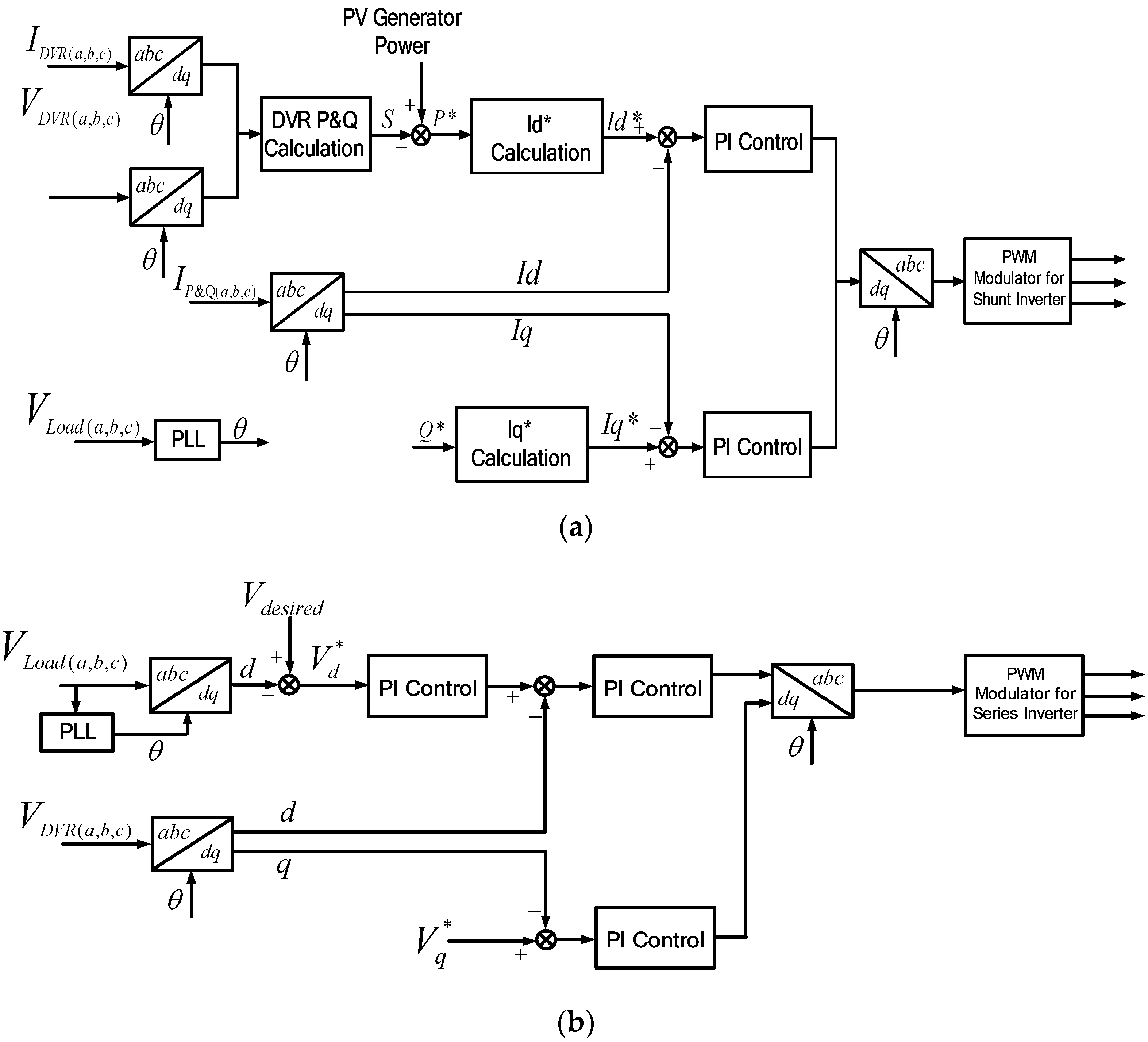
Figure 7a,b shows the control blocks for voltage compensation. Figure 7a shows the control scheme for shunt inverter. The reference currents, I*d and I*q, are generated to deliver the power through the shunt inverter, the same as the power difference between the PV generated power and the power delivered to the grid through the series inverter. Then the current-controlled PWM is applied to let the output current of shunt inverter, Id and Iq, follow this reference value. On the other hand, the reference voltages, V*d and V*q, are generated to supply the compensation voltage, and the voltage-controlled PWM is applied to regulate the output voltage of the series inverter, Vd and Vq, to follow this reference value, as shown in Figure 7b. The power flow during this mode is shown in Figure 7c.
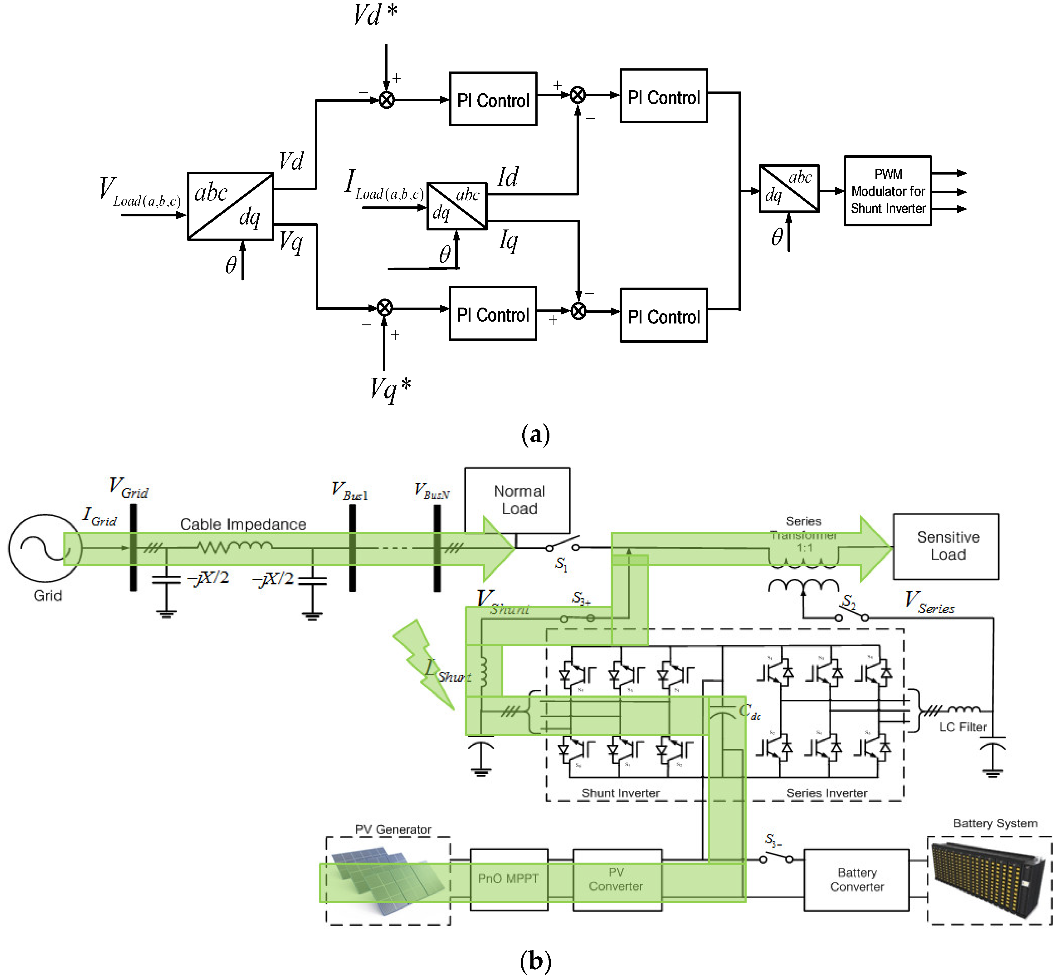
4.3. Stand-Alone Mode
When the line voltage is out of range for compensation, the static switch disconnects the sensitive load from the grid, and then the PV power is delivered to the load by the shunt inverter under the stand-alone mode without any voltage compensation by the series inverter, as shown in Figure 8a,b.
The load voltage, Vd and Vq, is controlled to follow the reference voltage, V*d and V*q. This controller is composed of the outer voltage controller and the inner current controller. Then, the output abc signals are fed to PWM to generate the gating pulses for the shunt inverter.
For transferring between the power control under the grid connected mode and the voltage control under the stand-alone mode, the multiplexer is installed before the dq to abc transformation. The multiplexer may multiply the signal in voltage control to be zero when the grid voltage is in the range of the grid connected. The same treatment can be applied in power control, so the multiplexer will make the power control signal have a zero value when the grid voltage is in the range of the stand-alone mode.
4.4. Voltage Compensation Mode from BESS
In low irradiance or at night, the PV cannot produce power, so the BESS system provides the power for the series inverter only as shown in Figure 9a,b. In undervoltage conditions, the BESS will not supply the power to the shunt inverter due to the limitations of BESS capacity. On the other hand, the BESS system supports the series inverter only to mitigate the voltage disturbance in this mode. The control scheme is the same as the voltage compensation mode of the series inverter; the only difference is the power source. In the voltage compensation mode with PV power, the power source is the PV power, but in this mode, the power source is the BESS power. The BESS capacity SoC in this simulation is assumed to be 1 or fully charged.
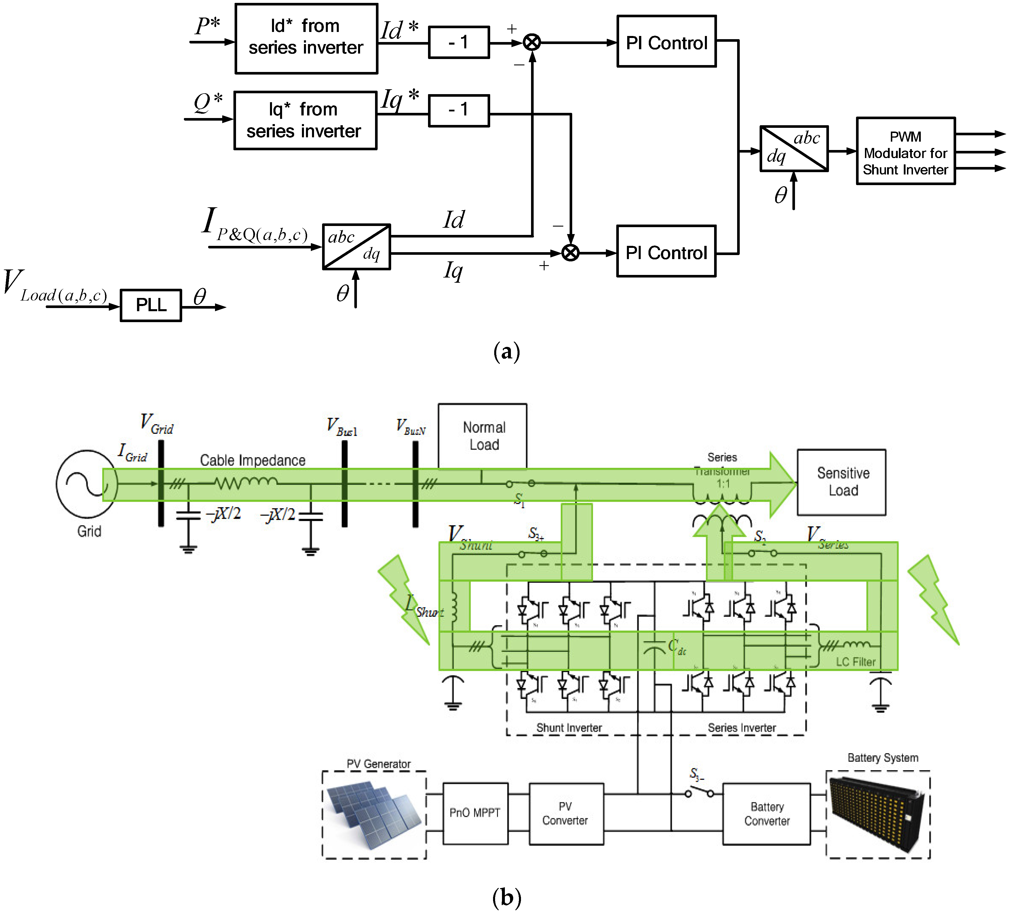
4.5. Voltage Compensation Mode from Grid
In this condition, we assumed that the BESS power almost reached 0.1 SoC. There will be times when the BESS cannot support the series inverter anymore. In this condition, the BESS switch will be turned off. The shunt inverter will be a load from the grid side to absorb the power and deliver it to the series inverter, as shown in Figure 10. Thus, the series inverter can compensate for the undervoltage in this condition. The control scheme for the series inverter is the same as the voltage compensation mode. For the shunt inverter, there are some modifications due to supply power to the series inverter. The power absorbed from this mode is based on the power required by the series inverter. Thus, the value of the power desired in this condition is based on Equations (11) and (12), which will be determined by the demand from the series inverter.
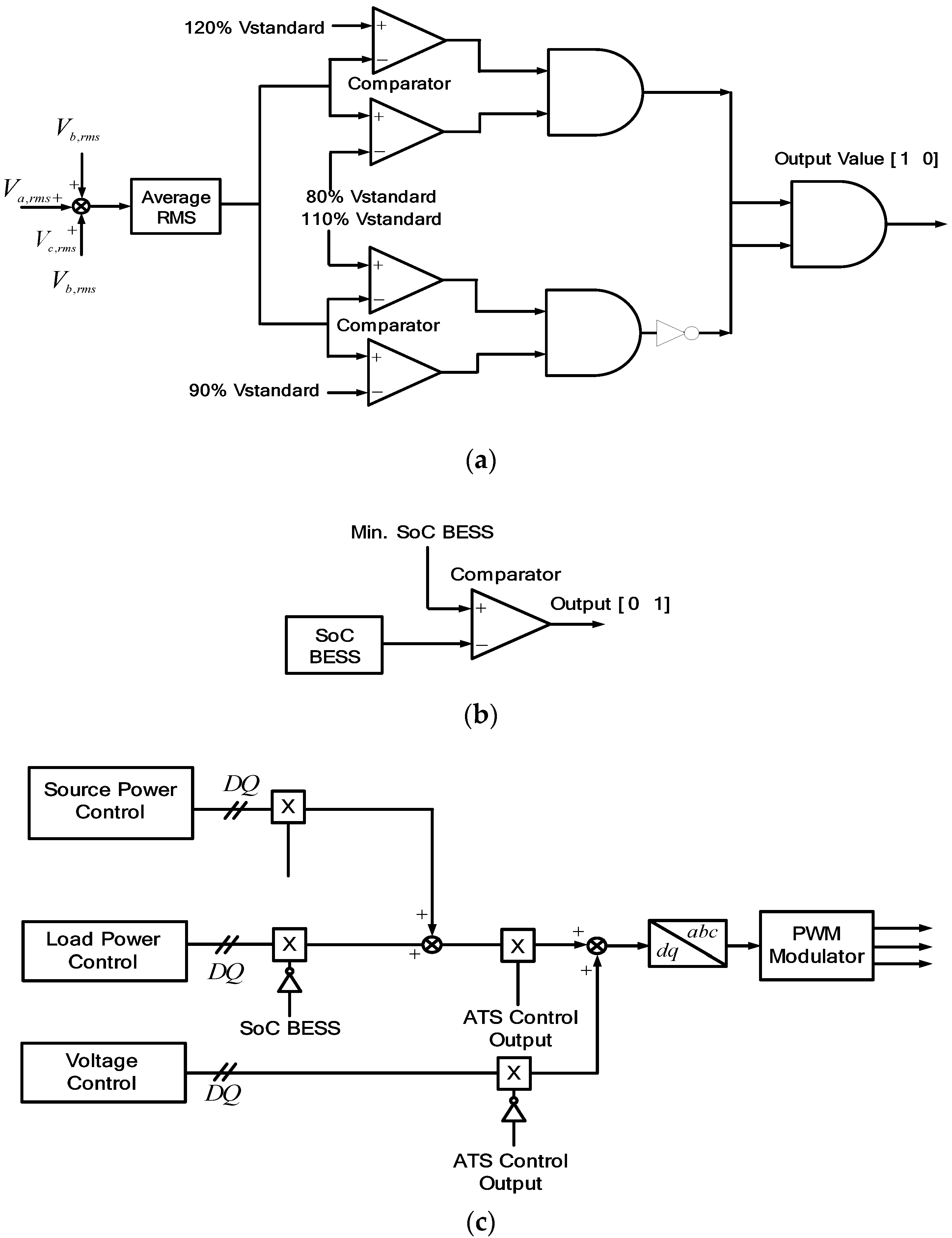
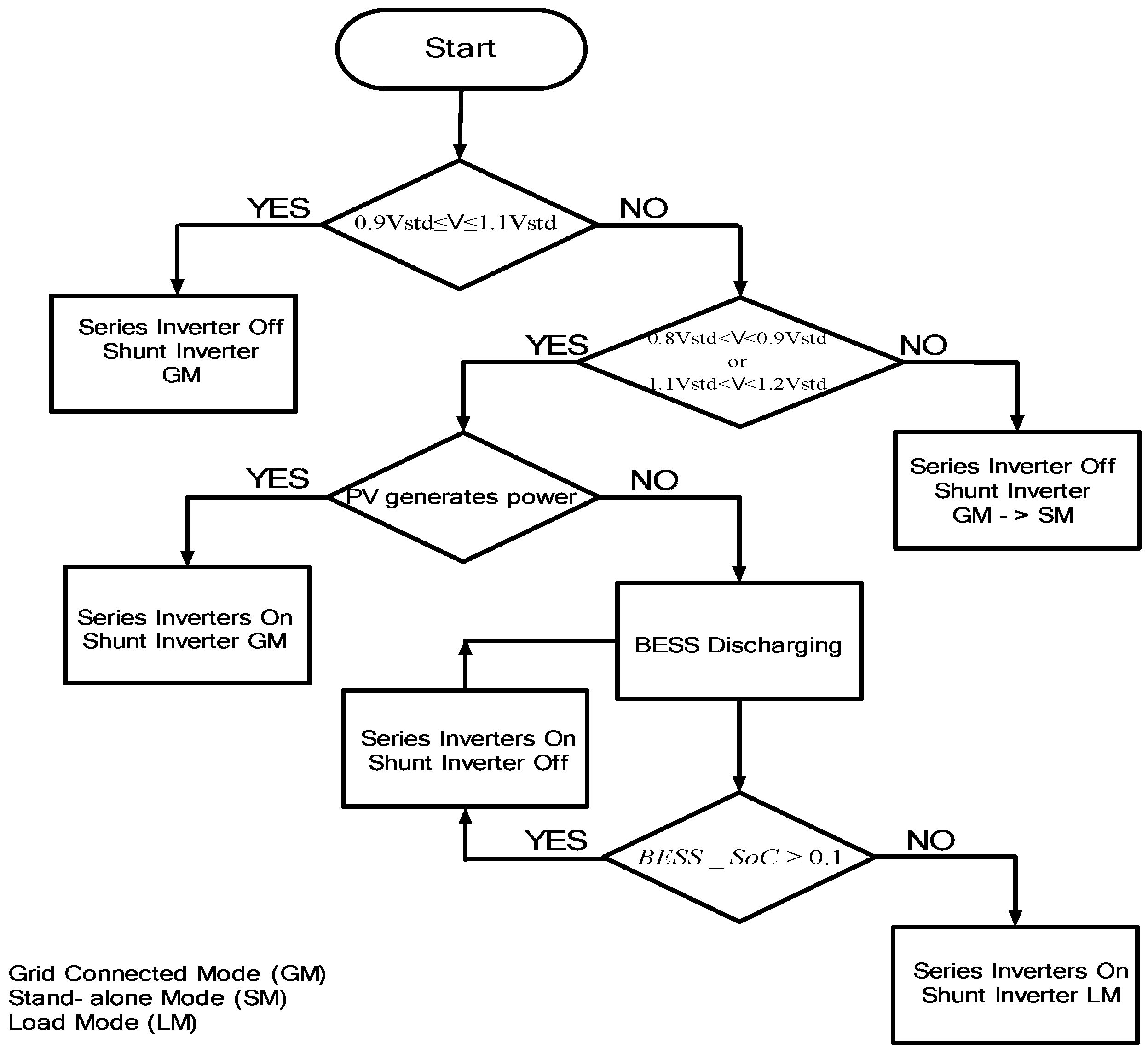
4.6. Automatic Transfer Switches
There are four switches in this proposed scheme. Switch 1, S1, is located between the grid and the sensitive load; Switch 2, S2, is between the series inverter and the sensitive load; Switch 3, S3+, is between the shunt inverter and the grid; and Switch 4, S3-, is between the BESS and inverters, respectively. The control scheme of switches for series and shunt inverters are based on the value of the grid voltage. If the sensitive load voltage is 0.9 to 1 pu, S1 is turned on. The shunt inverter is connected to the grid and supplies the power to the sensitive load without voltage compensation, as shown in Figure 11a,c. If the voltage magnitude is 0.8 to 0.9 pu, Switch S2 is turned on and the voltage compensation is applied by the series inverter, while the shunt inverter delivers the generated PV power to the grid through the shunt inverter. If the line voltage is lower than 0.8pu rated voltage, then both S1 and S2 are turned off, as shown in Figure 11a, to separate the sensitive load from the normal load. Then it operates as the stand-alone mode and the shunt inverter supplies the power directly to the sensitive load under the voltage control, while the normal load is supplied power from the grid with poor power quality.
The same control strategy can be applied for overvoltage condition. If the line voltage is between 1.1 and 1.2 pu, Switches S1 and S2 are turned on and the series inverter compensates for the overvoltage while the shunt inverter delivers the PV power to the grid. When the line voltage is higher than 1.2 pu, Switches S1 and S2 are turned to the off position and the stand-alone mode is applied, the same as in undervoltage conditions.
On the other hand, during a no PV generation condition, the BESS supports the series inverter without the operation of the shunt inverter by turning off Switch S3-. However, when the SoC of BESS is lower than 0.1, the shunt inverter absorbs the power from the grid to support the series inverter by turning on Switch S3+.
5. Simulation Results and Discussion
5.1. Simulation Conditions and Parameters
In this simulation, the PV with MPPT model, the series inverter, the shunt inverter, the grid, and the loads are presented. Table 1 and Figure 12 present the simulation parameters and the system operation flowchart for PSIM simulation. The PV model is implemented by using the physical model, which is available in PSiM software (version, city country). The BESS is lithium-ion and the model is available in PSiM software.
Each case has been tested in several conditions. For the undervoltage case, the normal condition is shown first, followed by the grid undervoltage between 0.8 to 0.9 pu and the stand-alone mode, which is the grid undervoltage less than 0.8pu. For the overvoltage, the normal condition is presented from t < 1 s, followed by the grid overvoltage in the range of 1 to 1.1 pu and the stand-alone mode when the grid voltage is more than 1.1 pu.
The next case is the voltage compensation without PV power mode. In this condition, it is assumed that the BESS can supply the power to the series inverter, so the BESS generates the power to the series inverter only for voltage compensation. The last case is when the BESS cannot support the series inverter anymore, so the shunt inverter delivers the power from the grid to the series inverter.
5.2. Undervoltage Case
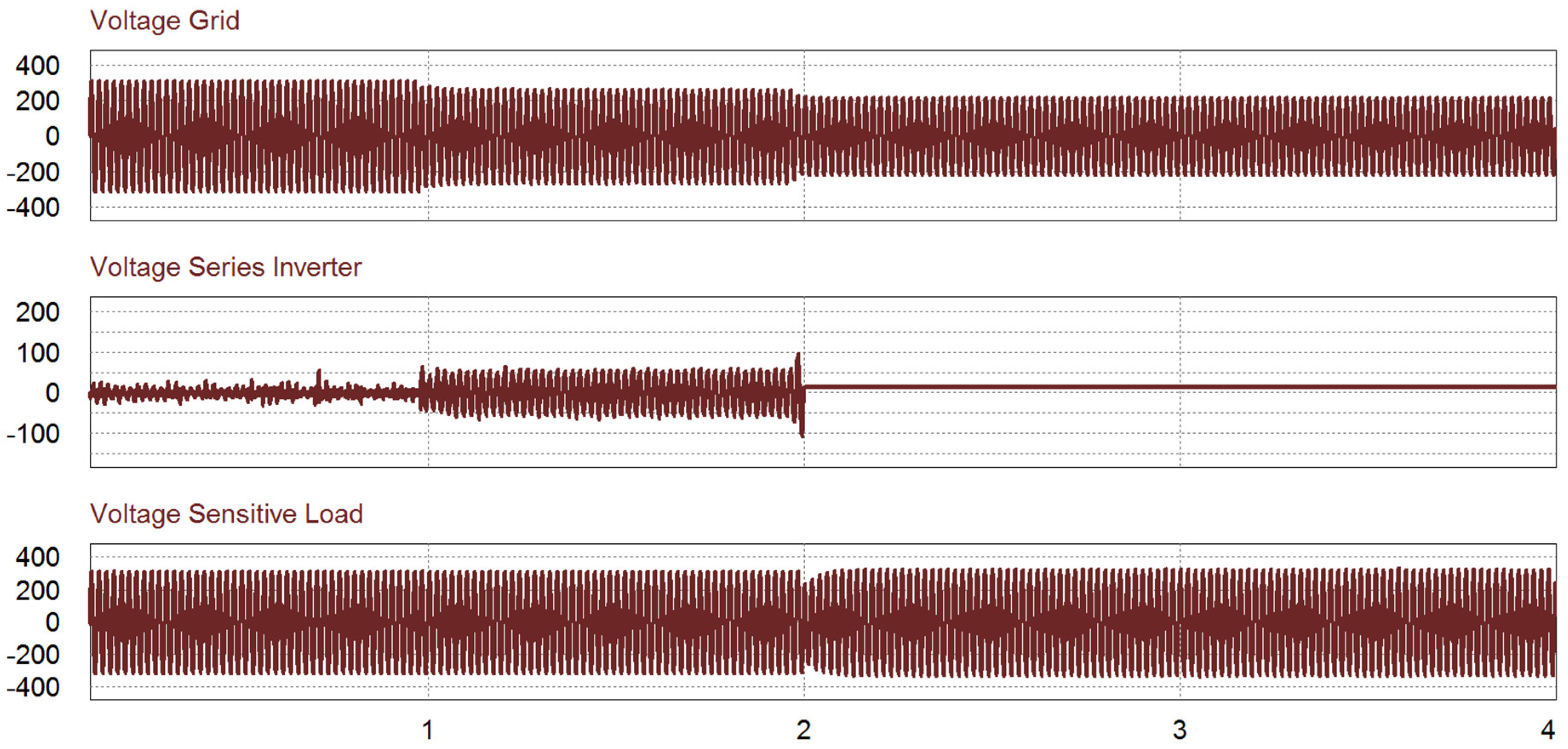
In this simulation, there are three cases within certain periods, as shown in Figure 13. Before 1 s, no undervoltage occurred. Therefore, there is no action from the series inverter while the shunt inverter injects the active power to the grid. During 1 < t < 2 s, the undervoltage occurs under 0.9 pu. The switch S2 is turned on and the series inverter injects the voltage to compensate for the grid voltage. After t > 2 s, if the voltage is lower than 0.8 pu, the shunt inverter takes care of the sensitive load in stand-alone mode while the grid covers the normal load in grid mode. In Figure 13c, it is verified that the voltage waveform of the sensitive load is well regulated during the undervoltage condition by the voltage compensation of the series inverter. In this period, the shunt inverter control is transferred from the power control mode to the voltage control mode.
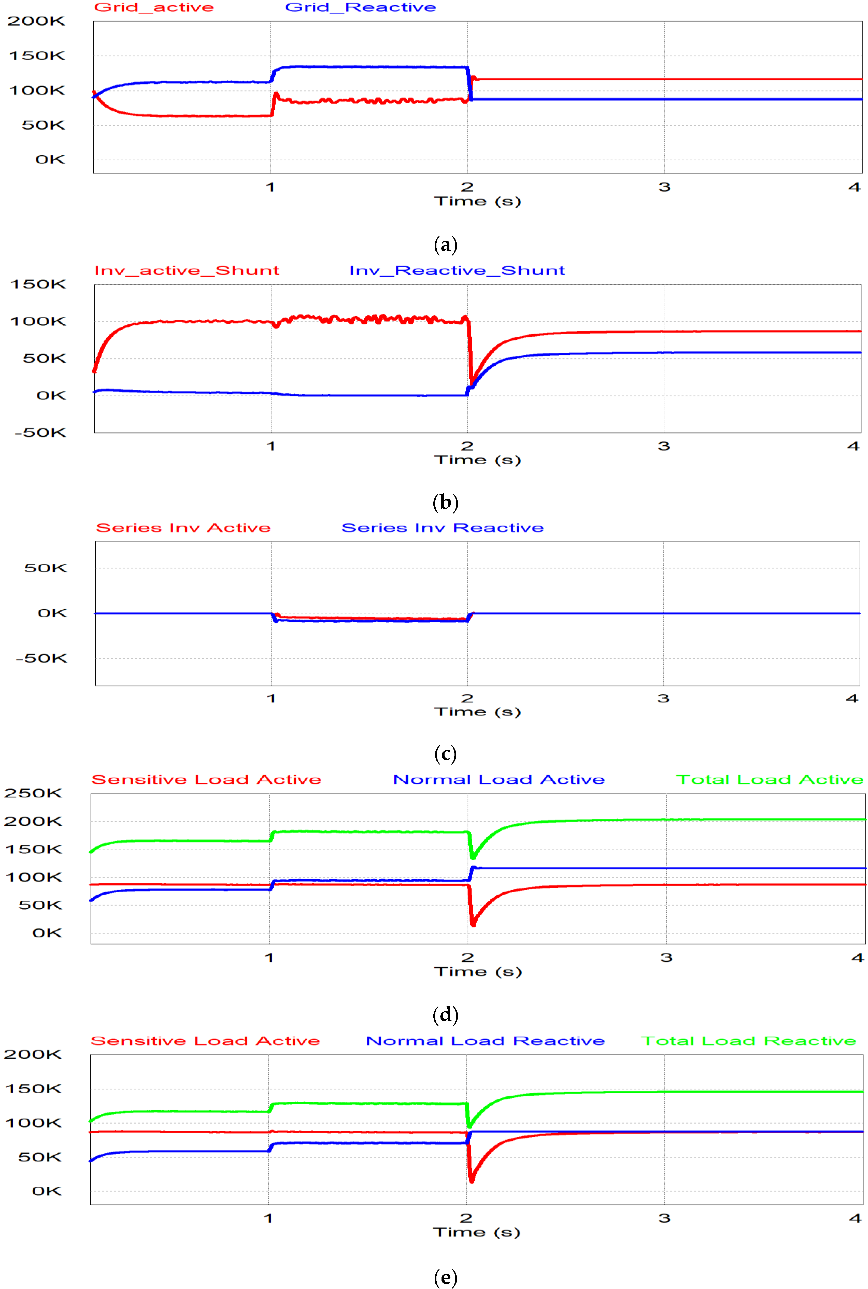
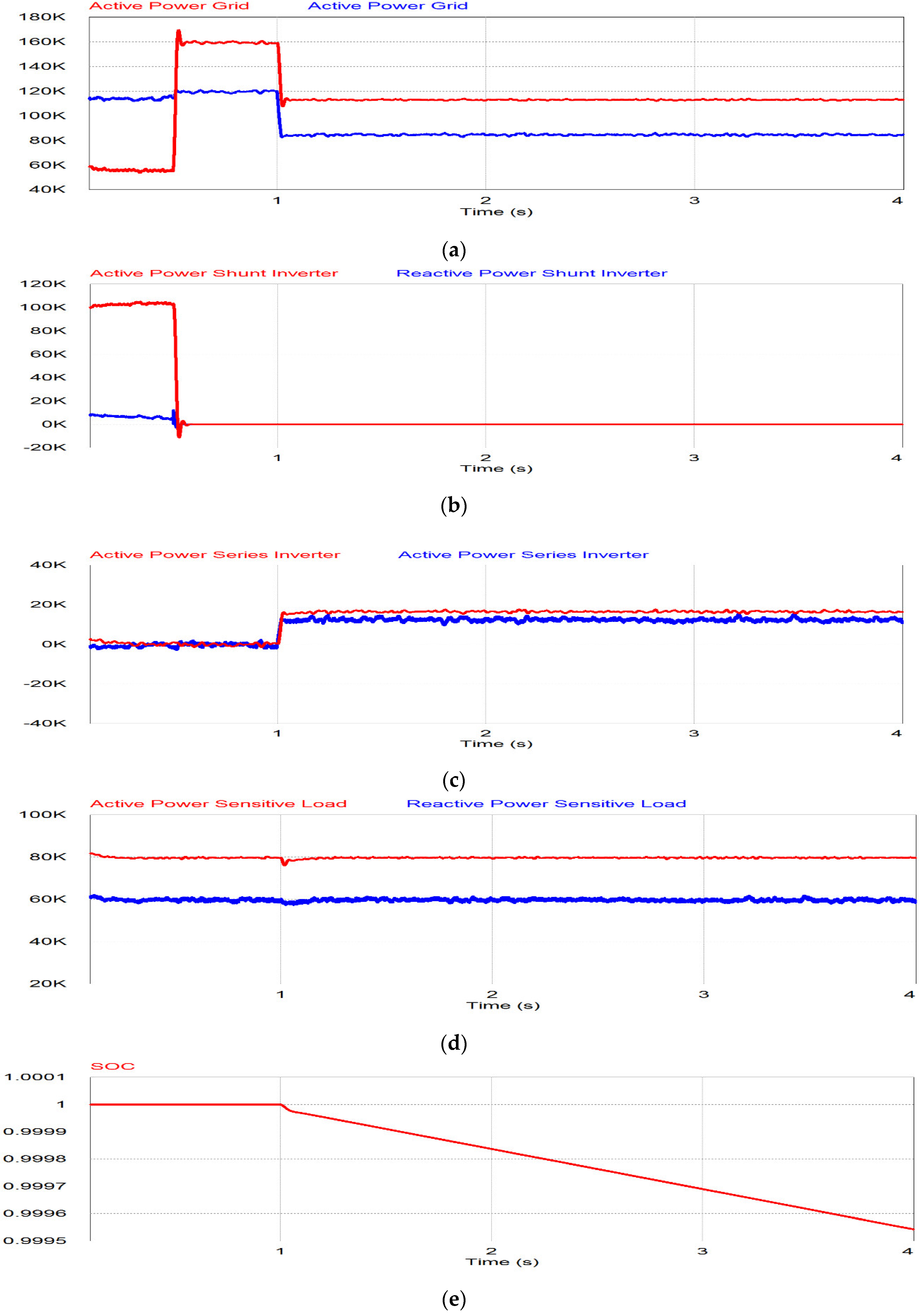
The simulation results for power flow are shown in Figure 14. During the period t < 1 s, the grid injects power for the normal condition as shown in Figure 14a. In Figure 14b,c, there is no power flow through the series inverter, which is in the off position, but the shunt inverter injects the active power generated by PV to the grid system. When undervoltage occurs during 1 < t < 2 s, the grid power is decreased due to the voltage drop, as shown in Figure 14a. The series inverter injects the power to compensate for the undervoltage, while the remaining PV generating power flows through the shunt inverter, as shown in Figure 14b,c. The active and reactive power of sensitive load are constant in this period since the series inverter compensates for the undervoltage through the series inverter as shown in Figure 14d,e. During the last period (t > 2 s), the grid voltage is less than 0.8 pu. The series inverter is in off mode and the shunt inverter takes care of the sensitive load in the stand-alone mode. Therefore, the normal load is covered by the grid as shown in Figure 14a,d,e, while the shunt inverter supplies the power to the sensitive load, separate from the normal load, as shown in Figure 14c–e.
5.3. Overvoltage Case
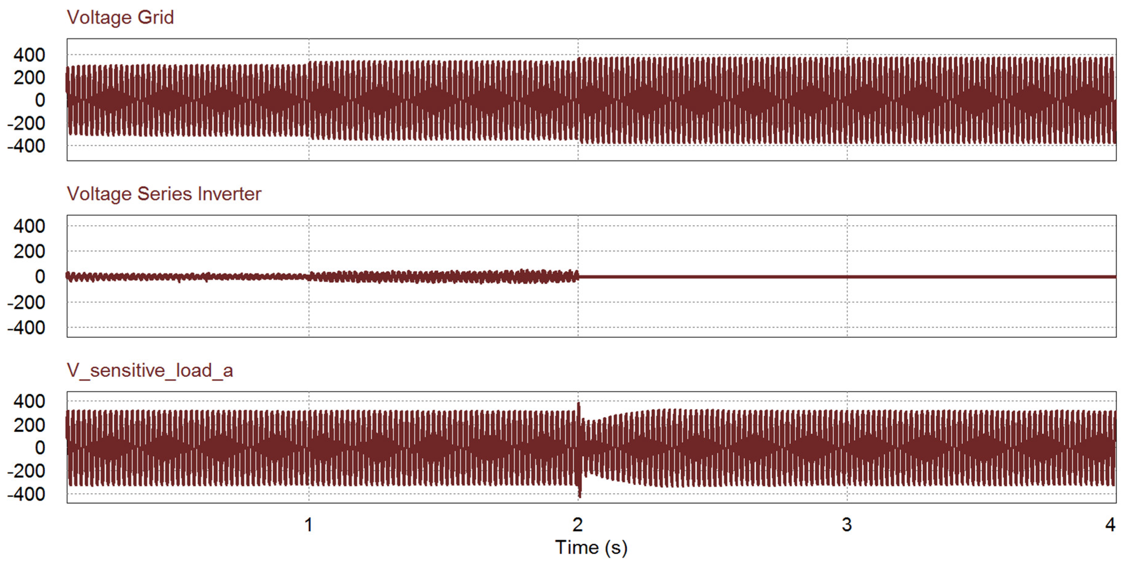
The performance analysis in the overvoltage case is applied in reverse to the under–voltage case. As shown in Figure 15, the series inverter does not operate under the normal before 1 s while the shunt inverter injects the active power to the grid. During 1 < t < 2 s, the overvoltage occurs over 1.1 pu, then the series inverter compensates for the voltage by absorbing the power from the grid. After t > 2 s, the voltage is higher than 1.2 pu, then the shunt inverter keeps the voltage for the sensitive load in stand-alone mode. In Figure 15c, it is verified that the voltage waveform of sensitive load is well regulated during the overvoltage condition by the voltage compensation of the series inverter.
The power flow under the overvoltage case is same as that of undervoltage case as shown in Figure 16. Before 1 s, the grid is under the normal condition, so there is no power flow through the series inverter while the shunt inverter injects the generated PV power to the grid system. When the overvoltage occurs during 1 < t < 2 s, the series inverter compensates for the voltage while the remaining PV generating power flows through the shunt inverter as shown in Figure 16b,c. The active and reactive power of sensitive load is constant in this period since the series inverter compensates for the overvoltage through the series inverter as shown in Figure 16d,e. During the last period (t > 2 s), the grid voltage is higher than 1.2 pu. The series inverter is in off mode and the shunt inverter takes care of the sensitive load in the stand-alone mode. Therefore, the normal load is covered by the grid as shown in Figure 16a,d,e, while the shunt inverter supplies the power to the sensitive load only, as shown in Figure 16c‒e.
5.4. Voltage Compensation without PV Power Case
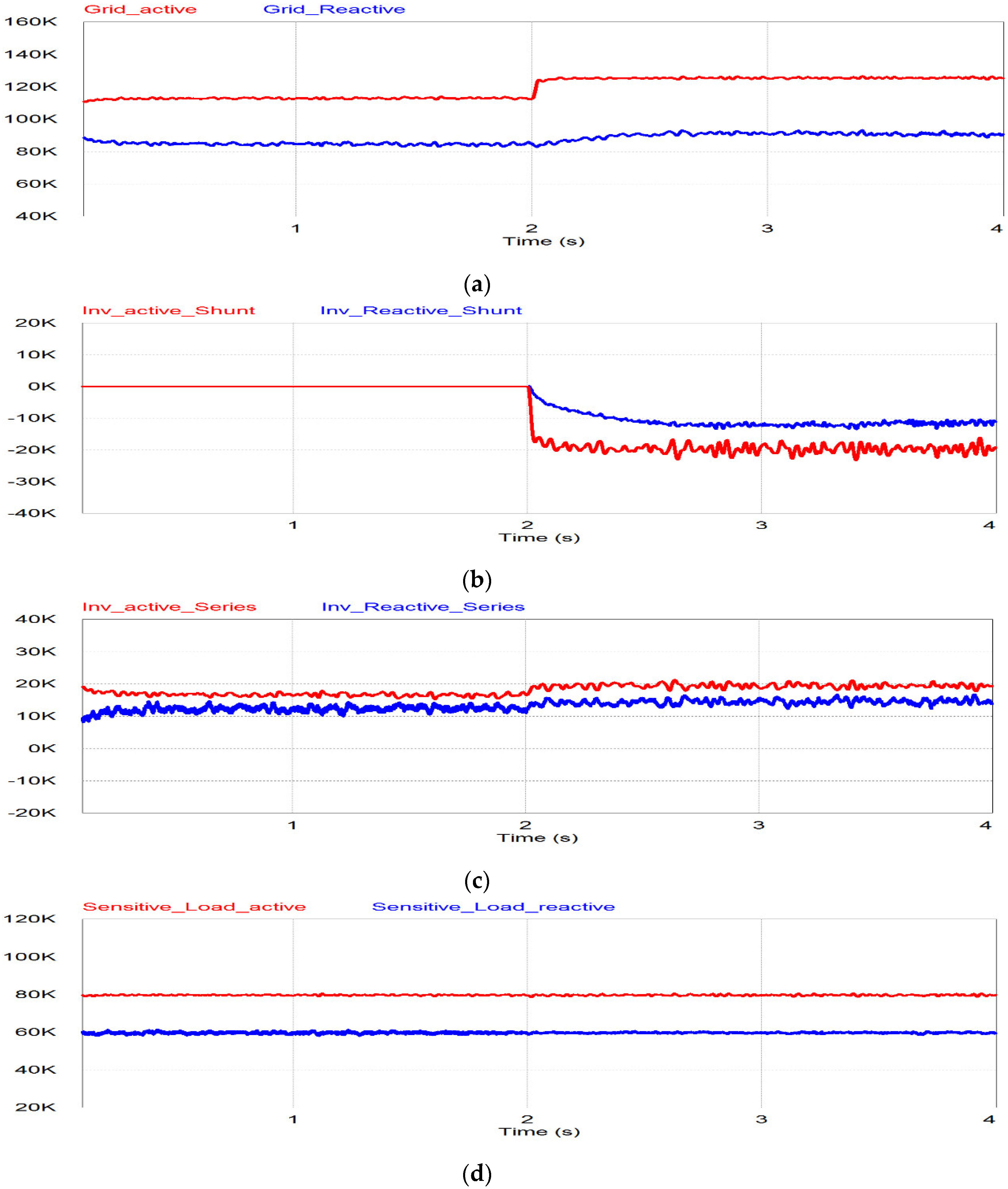
This case is the condition of low irradiance or during the night. Figure 17a shows the voltage compensation after 1 s by discharging the battery. Before 0.5 s, the PV-generated power is supplied to the grid through the shunt inverter, so the grid injects less active power to the grid due to the power delivery of shunt inverter shown in Figure 17a‒c. During 0.5 to 1.0 s, the PV cannot generate active power due to the low irradiance condition and the grid injects more power to the loads shown in Figure 17a. After t > 1.0 s, undervoltage occurs, so the BESS supplies power to the series inverter to compensate for the voltage shown in Figure 17b,c. The active and reactive power for the sensitive load can stay constant, as shown in Figure 17d. During this range, the BESS can be the power source of the series inverter instead of the PV power source, so the SoC of BESS is reduced due to the power supply to the series inverter, as shown in Figure 17e.
5.5. Voltage Compensation with Power from Grid Case
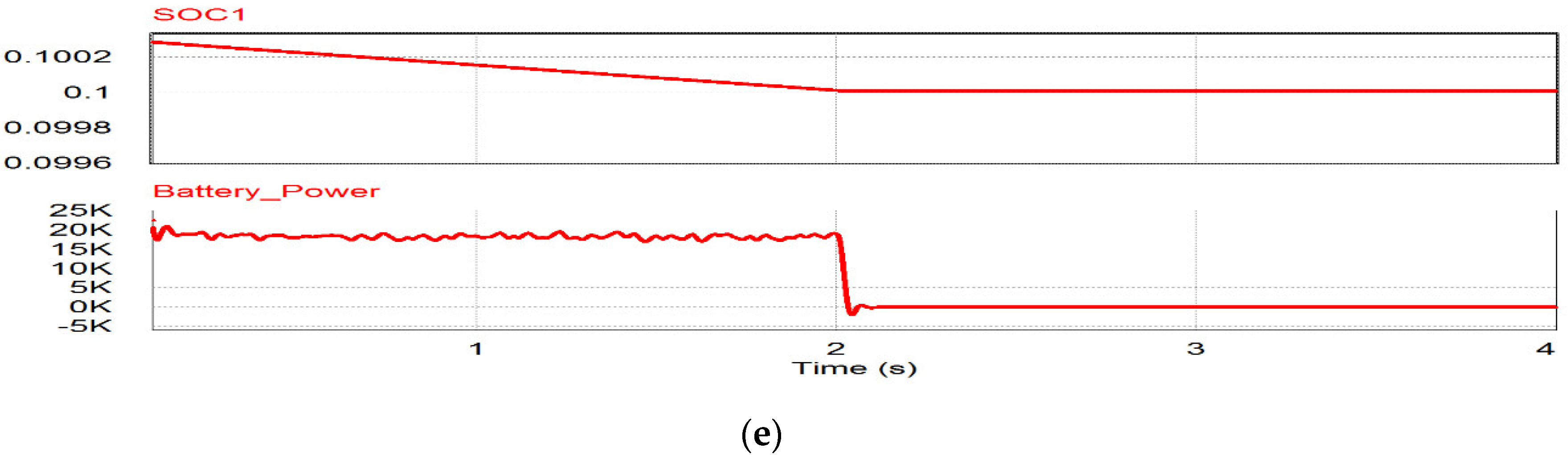
The last mode is the voltage compensation with the grid power mode as shown in Figure 18 and the continuation of the case after the voltage compensation without PV power case. Before t < 2 s, the BESS has to support the series inverter due to no PV power generation as shown in Figure 18b,e, and the response is the same of the voltage compensation without PV power after 1 s. Switch S3+ is in the off position and Switch S3- is in the on position. The grid still supplies the sensitive load, though the grid voltage is in the undervoltage condition, as shown in Figure 18a,d. When the SoC of BESS reaches 0.1, as shown in Figure 18e, the BESS cannot supply the power to the series inverter anymore under the assumption of the Depth of Discharge (DoD) BESS of 0.1. When the DoD of BESS is less than 0.1, the shunt inverter will act as a load to the grid. Therefore, the shunt inverter absorbs the power from the grid and delivers it to the series inverter and the series inverter compensates for the load voltage as shown in Figure 18c. The control of the shunt inverter will be transferred to the load mode. The power absorbed from the shunt inverter will be delivered to the DC capacitor to keep the voltage constant. In Figure 18b, it is shown that during t > 2 s the undervoltage is worse due to the additional load from the shunt inverter. The loads will increase because of the shunt inverter as an additional load and due to that the undervoltage will increase too. That is why the series inverter injects more voltage to compensate for the grid voltage after t > 2 s.
6. Conclusions
This paper proposes multi-functional PV inverters based on the UPQC configuration in which the back-to-back inverters are connected to the grid by series and shunt. The line voltage is compensated for by the series inverter, while the shunt inverter delivers the PV generating power to the grid. From the point of view of voltage compensation, it has been compared to the conventional DVR, which can be divided by the external voltage compensator for the distributed generating system. The UPQC configuration has been used in place of the conventional grid-connected inverter and the external DVR for the compensation of voltage while delivering the PV generating power. Finally, the microgrid concept has been applied to keep the different power quality levels depending on the importance of the loads.
Depending on the grid voltage and the condition of weather and battery SOC, it can operate in one of five different modes: normal mode, voltage compensation mode, stand-alone mode, voltage compensation mode from BESS and voltage compensation mode from grid. The operation performance at each mode is analyzed by using the PSiM simulation with the voltage waveforms and the active and reactive power flows. From the simulation results, the proposed idea is well verified so that it can be applied for the power quality improvement of a weak grid power system such as in isolated areas or on islands connected to the mainland by long submarine cables.
Author Contributions
Conceptualization and Methodology, D.P.S. and J.C.; Software, Validation, and Writing-Original Draft Preparation, D.P.S.; Writing-Review, Editing and Supervision, J.C.
Acknowledgments
This work was supported by the Korea Institute of Energy Technology Evaluation and Planning (KETEP) and the Ministry of Trade, Industry & Energy (MOTIE) of the Republic of Korea (No. 20171210200840).
Conflicts of Interest
The authors declare no conflict of interest.
References
- United Nations. Kyoto Protocol to the United Nations Framework Convention on Climate Change; United Nations: New York, NY, USA, 1998. [Google Scholar]
- IEA International Energy Agency. Snapshot of Global Photovoltaic Markets: Report IEA PVPS T1-33. 2018. Available online: http://www.iea-pvps.org/fileadmin/dam/public/report/statistics/IEA-PVPS_-_A_Snapshot_of_Global_PV_-_1992-2017.pdf (accessed on 8 July 2018).
- Guide for Planning DC Links Terminating at AC Systems Locations Having Low Short-Circuit Capacities, Part I: AC/DC Interaction Phenomena; IEEE Std. 1204-1997; IEEE: Piscataway, NJ, USA, 1997.
- Keyhani, A. Design of Smart Power Grid Renewable Energy Systems, 2nd ed.; Wiley-IEEE Press: Piscataway, NJ, USA, 2015. [Google Scholar]
- IEEE Recommended Practice for Monitoring Electric Power Quality; IEEE Std. 1159-2009; IEEE: Piscataway, NJ, USA, 1999.
- Nagpal, M.; Martinich, T.G.; Bimbhra, A.; Sydor, D. Damaging open-phase overvoltage disturbance on a shunt-compensated 500-kV line initiated by unintended trip. IEEE Trans. Power Deliv. 2015, 30, 412–419. [Google Scholar] [CrossRef]
- Chavan, G.; Acharya, S.; Bhattacharya, S.; Das, D.; Imam, H. Application of static synchronous series compensators in mitigating Ferranti effect. In Proceedings of the 2016 IEEE Power and Energy Society General Meeting (PESGM), Boston, MA, USA, 1–5 July 2016. [Google Scholar]
- Natesan, C.; Ajithan, K.; Palani, P.; Kandhasamy, P. Survey on microgrid: Power quality improvement techniques. Renew. Energy 2014, 342019. [Google Scholar] [CrossRef]
- AppalaNaidu, T. The Role of Dynamic Voltage Restorer (DVR) in improving power quality. In Proceedings of the 2016 International Conference on Advances in Electrical, Electronics, Information, Communication and Bio-Informatics (AEEICB), Chennai, India, 27–28 February 2016. [Google Scholar]
- Fernandes, D.; Costa, F.; Martins, J.; Lock, A.; Silva, E.; Vitorino, M. Sensitive load voltage compensation Performed by a Suitable Control Method. IEEE Trans. Ind. Appl. 2017, 53, 4877–4885. [Google Scholar] [CrossRef]
- Sin, C.; Choi, J. Compensation of current harmonics caused by local nonlinear load for grid-connected converter. In Proceedings of the IFEEC 2017-ECCE Asia, Kaohshiung, Taiwan, 3–7 June 2017. [Google Scholar]
- Jayaprakash, P.; Singh, B.; Kothari, P.; Chandra, A.; Al-Haddad, K. Control of reduced-rating dynamic voltage restorer with a battery energy storage system. IEEE Trans. Ind. Appl. 2014, 50, 1295–1303. [Google Scholar] [CrossRef]
- Gee, A.; Robinson, F.; Yuan, W. A Superconducting magnetic energy storage-emulator/battery supported dynamic voltage restorer. IEEE Trans. Energy Convers. 2017, 32, 55–64. [Google Scholar] [CrossRef]
- Choi, S.; Li, J.; Vilathgamuwa, D. A generalized voltage compensation strategy for mitigating the impacts of voltage sags/swells. IEEE Trans. Power Deliv. 2005, 20, 2289–2297. [Google Scholar] [CrossRef]
- Khadkikar, V. Enhancing electric power quality using UPQC: A comprehensive overview. IEEE Trans. Power Electron. 2012, 27, 2284–2297. [Google Scholar] [CrossRef]
- Graovac, D.; Katic, V.; Rufer, A. Power quality compensation using universal power quality conditioning system. IEEE Power Eng. Rev. 2000, 20, 58–60. [Google Scholar]
- Somayajula, D.; Crow, M. An integrated dynamic voltage restorer-ultracapacitor design for improving power quality of the distribution grid. IEEE Trans. Sustain. Energy 2015, 6, 616–624. [Google Scholar] [CrossRef]
- Karimian, M.; Jalilian, A. Proportional-repetitive control of a dynamic voltage restorer (DVR) for power quality improvement. In Proceedings of the 17th Conference Electrical Power Distribution, Tehran, Iran, 1–6 May 2012. [Google Scholar]
- Fernandes, D.; Costa, F.; Martins, J.; Lock, A.; Silva, E.; Vitorino, M. Sensitive load voltage compensation with a suitable control method. In Proceedings of the IEEE Energy Conversion Congress Exposition, Montreal, QC, Canada, 20–24 September 2015. [Google Scholar]
- Balaguer, I.; Lei, Q.; Yang, S.; Supatti, U.; Peng, F. Control for grid-connected and intentional islanding operations of distributed power generation. IEEE Trans. Ind. Electron. 2011, 58, 147–157. [Google Scholar] [CrossRef]
- Ramadesigan, V.; Northrop, P.; De, S.; Santhanagopalan, S.; Braarz, R.; Subramanian, V. Modeling and simulation of lithium-ion batteries from a system engineering perspective. J. Electrochem. Soc. 2012, 159, R31–R45. [Google Scholar] [CrossRef]
- Domenico, D.; Creef, Y.; Prada, E.; Duchene, P.; Bernard, J.; Sauvan-Moynot, V. A review of approaches for the design of Li-ion BMS estimation functions. J. Oil Gas Sci. Technol. 2013, 68, 127–135. [Google Scholar] [CrossRef]
- Grainger, J.; William, D.S. Power System Analysis; McGraw-Hill Inc.: New York, NY, USA, 1994. [Google Scholar]
- Song-Manguelle, J.; Harfman, T.M.; Chi, S.; Gunturi, S.K.; Datta, R. Power transfer capability of HVAC cable for subsea transmission and distribution system. IEEE Trans. Ind. Appl. 2014, 50, 2382–2391. [Google Scholar] [CrossRef]
- Jothibasu, S.; Mishra, M.A. Control scheme for storageless DVR based on characterization of voltage sags. IEEE Trans. Power Deliv. 2014, 29, 2261–2269. [Google Scholar] [CrossRef]
- Nielsen, J.G.; Blaabjerg, F. A detailed comparison of system topologies for dynamic voltage restorers. IEEE Trans. Ind. Appl. 2015, 41, 1272–1280. [Google Scholar] [CrossRef]
- Woodley, N.H.; Morgan, L.; Sundaram, A. Experience with an inverter-based dynamic voltage restorer. IEEE Trans. Power Delivery 1999, 14, 1181–1186. [Google Scholar] [CrossRef]
- Sanchez, P.; Acha, E.; Calderon, J.; Feliu, V.; Cerrada, A. A versatile control scheme for a dynamic voltage restorer for power quality improvement. IEEE Trans. Power Delivery 2009, 24, 277–284. [Google Scholar] [CrossRef]
- Lam, C.S.; Wong, M.C.; Han, Y.D. Voltage swell and overvoltage compensation with unidirectional power flow controlled dynamic voltage restorer. IEEE Trans. Power Delivery 2008, 23, 2513–2521. [Google Scholar]
- Sadigh, A.; Smedley, K. Review of voltage compensation methods in dynamic voltage restorer DVR. In Proceedings of the IEEE Power and Energy Society General Meeting, San Diego, CA, USA, 22–26 July 2012. [Google Scholar]
- Rauf, A.M.; Khadkikar, V. An enhanced voltage sag compensation scheme for dynamic voltage restorer. IEEE Trans. Ind. Electron. 2015, 62, 2683–2692. [Google Scholar] [CrossRef]
Figure 1.
Modeling of short and medium-length submarine cables.

Figure 2.
Distribution system submarine cable modeling without distributed generation (DG).

Figure 3.
Distribution system submarine cable modeling with DG.

Figure 4.
Proposed PV system for voltage compensation method.

Figure 5.
Phasor diagram for the series inverter: (a) overvoltage conditions; (b) undervoltage conditions.
Figure 5.
Phasor diagram for the series inverter: (a) overvoltage conditions; (b) undervoltage conditions.

Figure 6.
Normal mode: (a) Control scheme for shunt inverter; (b) power flow condition.

Figure 7.
Voltage compensation mode: (a) Control scheme for shunt inverter; (b) control scheme for series inverter; (c) power flow condition.
Figure 7.
Voltage compensation mode: (a) Control scheme for shunt inverter; (b) control scheme for series inverter; (c) power flow condition.


Figure 8.
Stand-alone mode: (a) Control scheme; (b) power flow condition.

Figure 9.
Voltage compensation mode from BESS: (a) Control scheme; (b) power flow condition.

Figure 10.
Voltage compensation mode from grid: (a) Control scheme; (b) power flow condition.

Figure 11.
Automatic transfer switches: (a) Series inverter; (b) BESS; (c) shunt inverter.

Figure 12.
Flowchart for proposed PV system for voltage compensation method.

Figure 13.
Simulation results of undervoltage case: (top) Grid voltage; (middle) series inverter voltage; (bottom) sensitive load voltage.
Figure 13.
Simulation results of undervoltage case: (top) Grid voltage; (middle) series inverter voltage; (bottom) sensitive load voltage.

Figure 14.
Simulation results of undervoltage: (a) Grid power; (b) shunt inverter power; (c) series inverter power; (d) active power for sensitive, normal and total load; (e) reactive power for sensitive, normal and total load.
Figure 14.
Simulation results of undervoltage: (a) Grid power; (b) shunt inverter power; (c) series inverter power; (d) active power for sensitive, normal and total load; (e) reactive power for sensitive, normal and total load.

Figure 15.
Simulation results of overvoltage case: (top) Grid voltage; (middle) series inverter voltage; (bottom) sensitive load voltage.
Figure 15.
Simulation results of overvoltage case: (top) Grid voltage; (middle) series inverter voltage; (bottom) sensitive load voltage.

Figure 16.
Simulation results of overvoltage: (a) Grid power; (b) shunt inverter power; (c) series inverter power; (d) active power for sensitive, normal and total load; (e) reactive power for sensitive, normal and total load.
Figure 16.
Simulation results of overvoltage: (a) Grid power; (b) shunt inverter power; (c) series inverter power; (d) active power for sensitive, normal and total load; (e) reactive power for sensitive, normal and total load.

Figure 17.
Simulation results of BESS: (a) Grid power; (b) shunt inverter power; (c) series inverter power; (d) active and reactive power for sensitive load; (e) SoC of BESS.
Figure 17.
Simulation results of BESS: (a) Grid power; (b) shunt inverter power; (c) series inverter power; (d) active and reactive power for sensitive load; (e) SoC of BESS.

Figure 18.
Simulation results of voltage compensation from grid power mode: (a) Grid power; (b) shunt inverter power; (c) series inverter power; (d) active and reactive power for sensitive load; (e) state of charge of BESS and BESS power.
Figure 18.
Simulation results of voltage compensation from grid power mode: (a) Grid power; (b) shunt inverter power; (c) series inverter power; (d) active and reactive power for sensitive load; (e) state of charge of BESS and BESS power.


Table 1.
Simulation parameters.
| Part of Circuit | Descriptions | Value |
|---|---|---|
| Grid | Main Voltage | 220; 190; 150 V |
| 220; 230; 264 V | ||
| Frequency | 50 Hz | |
| Battery | Capacity | 50 Ah |
| Undervoltage Load | Sensitive Load Active | 80 kW |
| Sensitive Load Reactive | 60 kVar | |
| Overvoltage Load | Sensitive Load Active | 72 kW |
| Sensitive Load Reactive | 50 kVar | |
| DC Capacitor | Capacity | Cdc = 10 mF |
| PV System | Max Power | 113 kW |
| Open Circuit Voltage | 684 V | |
| Short Circuit Current | 180 A | |
| Vmpp | 675 V | |
| Immp | 168 A | |
| Series Connection | Transformer | 1:1 |
| Filter | Cse = 50 µF, Lse = 1 mH | |
| PI-1, PI-2 & PI-3 | 20 | |
| Shunt Connection | Filter | Csh = 20 µF, Lsh = 2 mH |
| PI-1 & PI-2 (Power Control) | 200 | |
| PI-1 & PI-2 (Voltage and Load Mode) | 10 | |
| PWM | Sampling Frequency | 5 kHz |
© 2018 by the authors. Licensee MDPI, Basel, Switzerland. This article is an open access article distributed under the terms and conditions of the Creative Commons Attribution (CC BY) license (http://creativecommons.org/licenses/by/4.0/).
Share and Cite
MDPI and ACS Style
Simatupang, D.P.; Choi, J. Integrated Photovoltaic Inverters Based on Unified Power Quality Conditioner with Voltage Compensation for Submarine Distribution System. Energies 2018, 11, 2927. https://doi.org/10.3390/en11112927
AMA Style
Simatupang DP, Choi J. Integrated Photovoltaic Inverters Based on Unified Power Quality Conditioner with Voltage Compensation for Submarine Distribution System. Energies. 2018; 11(11):2927. https://doi.org/10.3390/en11112927
Chicago/Turabian StyleSimatupang, Desmon Petrus, and Jaeho Choi. 2018. "Integrated Photovoltaic Inverters Based on Unified Power Quality Conditioner with Voltage Compensation for Submarine Distribution System" Energies 11, no. 11: 2927. https://doi.org/10.3390/en11112927
Note that from the first issue of 2016, this journal uses article numbers instead of page numbers. See further details here.