Evaluation of Wind Resources and the Effect of Market Price Components on Wind-Farm Income: A Case Study of Ørland in Norway


Department of Energy and Power, Cranfield University, Bedfordshire MK43 0AL, UK
*
Author to whom correspondence should be addressed.
Energies 2018, 11(11), 2955; https://doi.org/10.3390/en11112955
Submission received: 30 September 2018
/
Revised: 22 October 2018
/
Accepted: 26 October 2018
/
Published: 29 October 2018
(This article belongs to the Special Issue Design, Fabrication and Performance of Wind Turbines 2019)
Abstract
:This paper aims to present a detailed analysis of the performance of a wind-farm using the wind turbine power measurement standard IEC61400-12-1 (2017). Ten minutes averaged wind data are obtained from LIDAR over the period of twelve months and it is compared with the 38 years’ data from weather station with the objective of determining the wind resources at the wind-farm. The performance of one of the wind turbines located in the wind-farm is assessed by comparing the wind power potential of the wind turbine with its actual power production. Our analysis shows that the wind farm under study is rated as ‘good’ in terms of wind power production and has wind power density of 479 W/m2. The annual wind-farm’s income is estimated based on the real-data collected from the wind turbines. The effect of price of electricity and the spot prices of Norwegian-Swedish green certificate on the income will be illustrated by means of a Monte-Carlo Simulation (MCS) approach. Our study provides a different perspective of wind resource evaluation by analyzing LIDAR measurements using Windographer and combines it with the lesser explored effects of price components on the income using statistical tools.
1. Introduction
The environmental concerns and global demand for clean energy have resulted in an increase in the number of wind energy projects throughout the world [1]. The EU has certain plans to expand the wind energy capacity to a point where 16.5% of all the electricity is produced from the wind energy by 2020 and more than half of new renewable energy installations to be for wind energy production [2]. The EU installed 15,638 MW new wind power capacity in 2017, which showed an increase of 25% compared with the year before [3]. The total EU wind power capacity by the end of 2017 reached 168.7 GW [3].
In order to speed up the development of wind energy in the EU, there is a need to analyze the wind resources of diverse geographical regions. A scheme to rezone potential wind resources world-wide based on cost, environmental risk and wind energy factors is discussed in [4]. Onea et al. [5] assessed the wind resources in the Black and Caspian seas by evaluating 12 years of wind data. The wind power density is an important assessment parameter indicating the wind energy potential of a given site. The wind direction is another factor used for positioning the wind turbines in the wind farm to maximize the power production. Nowadays, Laser Imaging Detection and Ranging (LIDAR) is extensively used for accurate site analysis and performance testing of wind turbines [6]. The benefits of using LIDAR technology over traditional met-masts are the ease of installation, higher resolution and the wider range [7].
A brief review of the literature shows that several studies have been carried out to estimate the resource potential of wind farms. The wind resource assessment and economics of electricity generation in the Sinai Peninsula of Egypt were studied by Ahmed [8]. Khan and Tariq [9] compared the wind resource assessment using Sonic Detection and Ranging (SODAR) with the metrological mast in Pakistan and concluded that wind resource assessment using SODAR is cheaper. The reliability of wind profiling using LIDAR is also discussed in [10]. Mifsud et al. [11] analyzed the performance of different Measure-Correlate-Predict (MCP) methodologies by gathering wind data from the LIDAR system. Fazelpour et al. [12] used the Windographer software [13] to perform wind resource analysis but they did not have access to the real wind data from LIDAR. Gleim et al. [14] dealt with uncertainties associated with the calculation of annual energy production using the MCS approach. They found that the wind speed uncertainty may cause error between 0.5% and 1.5% in estimation of annual energy production. Moreover, an MCS-based method to estimate annual energy production of wind farms was presented in [15].
The Tradable Energy Certificate (TGC) for the support of renewable energy in Norway and Sweden is discussed in details in [16]. Another study concludes that investment decisions are often made under considerable uncertainty because the market prices can change significantly with small changes in demand or supply [17]. Aune et al. [18] discussed the cost-effective distribution of renewable energy production and showed that TGCs would cut down the EU’s total cost of fulfilling the renewable energy target.
In this study, a detailed analysis of the wind resources of a small wind farm consisting of 3 wind turbines in Norway is performed using the standard IEC61400-12-1 [19], which extends the analysis presented in our earlier study [20]. This standard is proven to enhance the uniformity and precision in measurements and analysis of the power performance of the wind farm. As only a few months of data cannot be an indication of the actual potential of wind farms, the long-term potential of the site will be predicted using the MCP method. Then, the power potential of one of the wind turbines located in the wind-farm is compared with the actual power production and its performance will be evaluated. The actual power generated by the wind turbine is used to estimate the monthly income of the wind farm based on the Norwegian payment schemes. Our study is different from the previous studies in the sense that real wind data is obtained by placing a LIDAR on the wind farm rather than using weather station data, and we further use Windographer software to evaluate wind energy potential of the area. In addition, this study combines the detailed wind-farm analysis with the tradable electricity market in Norway and Sweden, and additionally uses MCS approach to evaluate the impact of electricity price and TGC price on the revenue of wind-farm.
2. Site Description
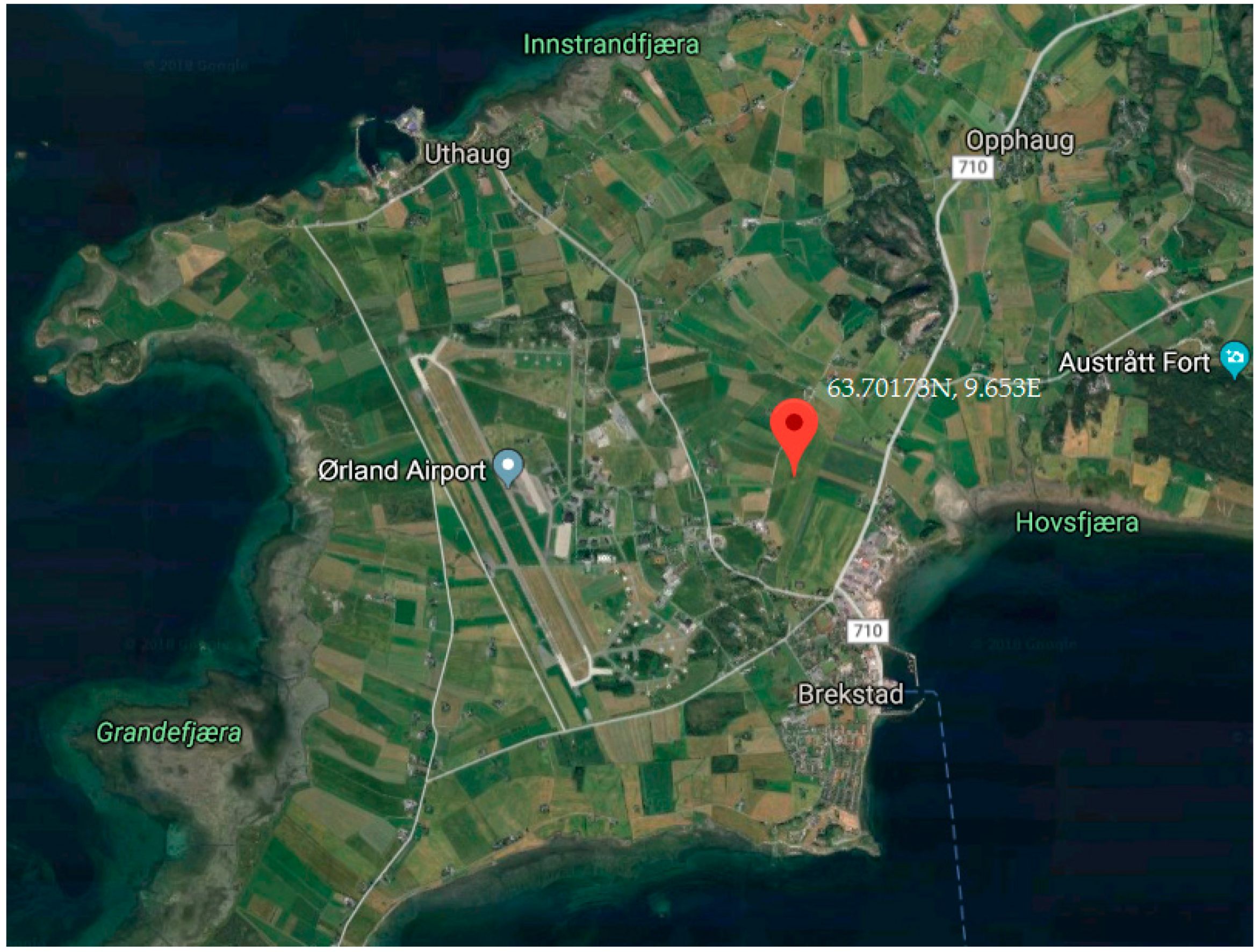
Ørland is situated in Sør-Trøndelag county, Norway, with an administrative centre in Brekstad city. It is situated on the northern coast of Trondheimsfjord and it further meets the Atlantic Ocean. The most of the terrain is uniform and distinctive from the rest of Norway in the way that only 2% of the city exceeds the height of 160 m above the sea level. It entails wide open spaces that are mainly used for agriculture and the main airbase of Norway (63.705 N, 9.6105 E).
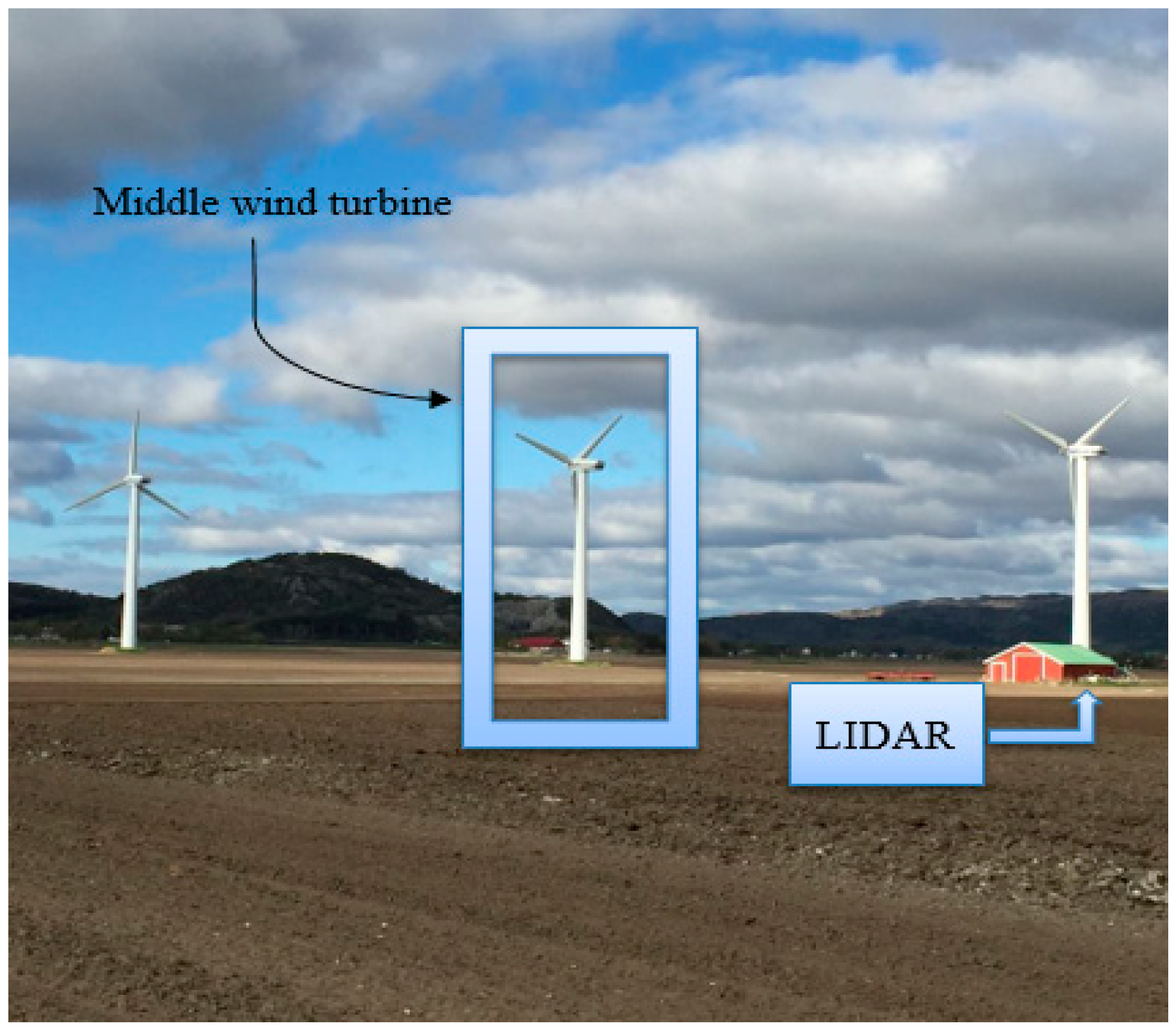
The wind farm chosen for this study consists of three Vestas V-27 wind turbines. The map of area around the wind farm is shown in Figure 1. Top view of the three wind turbines on the wind farm is also shown in Figure 2. On the site, there is a LIDAR system having exact coordinates of (63.70173 N, 9.653 E). The distance between LIDAR and the middle wind turbine is almost 112 m and the orientation is 18 degree. The LIDAR is located behind the shed as shown in Figure 3.
The Vestas V-27 is a horizontal axis wind turbine. It is a pitch regulated, upwind wind turbine with active yaw and its rotor has 3 blades [21]. The blades are manufactured with Glass Fiber Reinforced Polyester (GFRP), each comprising of two blade shells which are bonded on the supporting beam. The power is transmitted to the generator through two-stage gearboxes. The generator is asynchronous and is linked to the grid. To achieve maximum performance, the generator is changeable between eight poles and six poles generators. Based on the generator-1 or generator-2, the rotor rotates at two rotational speeds (43 RPM and 33 RPM, respectively).
It uses hydraulic disk brakes for the emergency stop, however full feathering is used for the braking purpose. The wind turbine is monitored and hence controlled by a control unit based on a microprocessor. Two wheel mounted yaw motors are placed on the top of turbine’s tower to achieve yawing. The nacelle is enclosed in a glass fiber reinforced cover and has an access through the central opening. There is a ladder for maintenance purposes inside the nacelle. The important specifications of Vestas V-27 wind turbine are listed in Table 1, while the specifications are given in detail in [22].
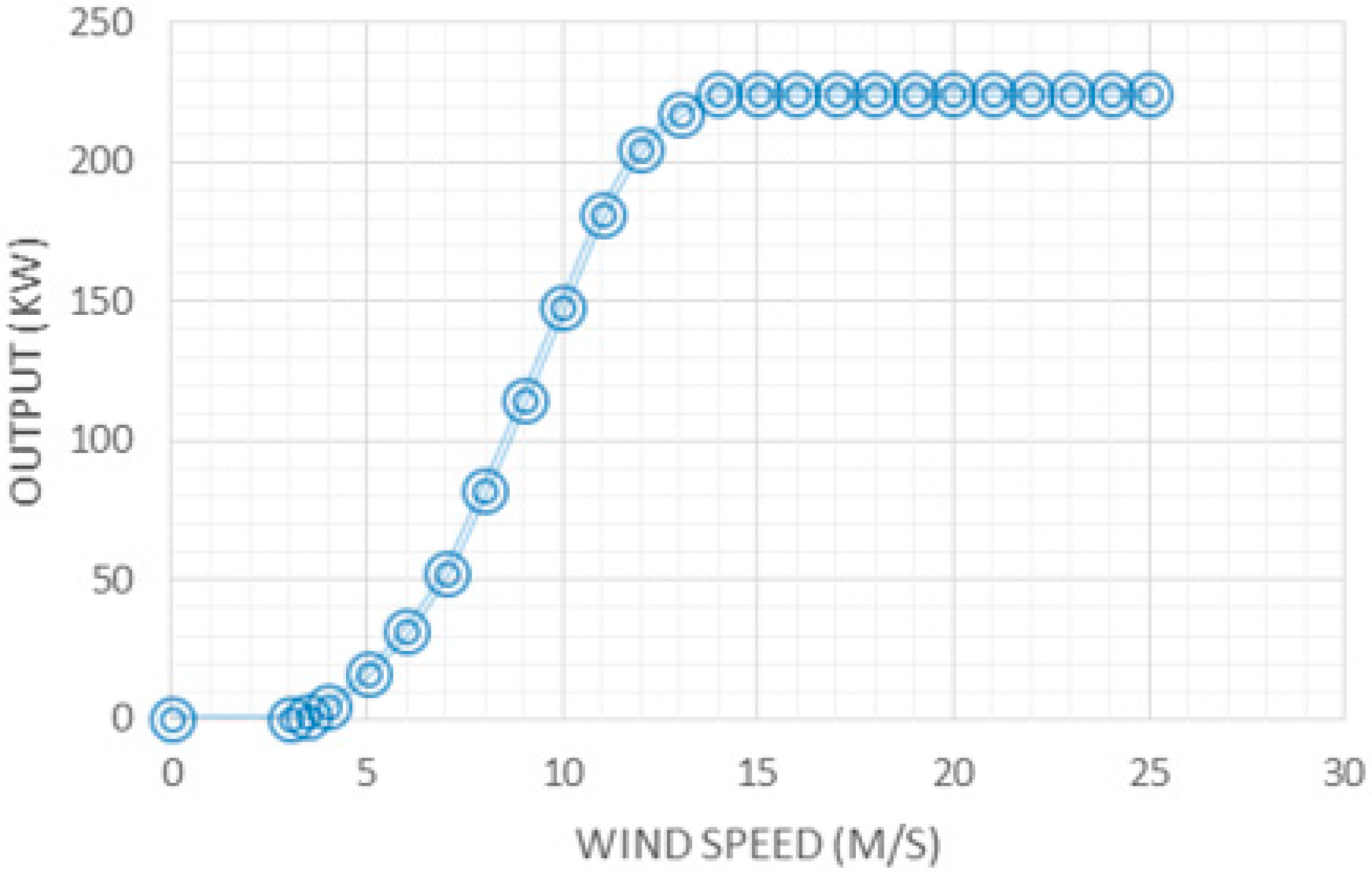
The power output data (as provided in [22]) versus given wind speeds at standard air density is illustrated in Figure 4.
As shown, the wind turbine approaches its rated power at the wind speed of 14 m/s. The power curve data is later used by the Windographer to estimate the performance of the wind turbine, using the wind data obtained from LIDAR.
3. Wind Resource Analysis
3.1. Theory
The power potential of any wind farm can be measured by performing wind resource analysis. There are many methods to model the wind speed over a time period but the most widely used technique is the Probability Density Function (PDF). The most common PDFs for the wind data analysis include Weibull and Rayleigh distributions. The Rayleigh distribution is based on only one parameter (mean wind speed), whereas the Weibull distribution is based on two parameters, namely scale, and shape, and hence, the Weibull distribution is more powerful and handy than one-parameter Rayleigh distribution. In this study, Weibull distribution is used for wind data analysis due to the better approximation using two parameters [23]. The general form of Weibull PDF is given as follows [24]:
where is the probability of observing the wind speed u, and k and c represent the scale and shape parameters of the Weibull PDF respectively. There are several methods in the literature for estimating parameters k and c. In this study, the Maximum Likelihood (ML) method is used because of its consistent approach to different parameter estimation problems. The ML estimators of parameters k and c are represented by the following equations:
where N is the number of samples and ui represents the ith observation in the sample.
3.2. Measurement Results
The LIDAR used for this study is WindCube V2. The LIDAR is capable of measuring wind profile up to the height of 200 m. However, the measurements from LIDAR includes some errors due to noise of the signal. The performance of ground based LIDAR was tested by Canadillas et al. [25]. She tested the performance of LIDAR by comparing the 10-min averaged data and compared it with the met-mast based instrumentation (cup anemometer). She found a high correlation (R2 = 0.99) between both the data sets, which recommends the use of LIDAR without the need to filter out these errors.
The IEC standard given in [19] also recommends using 10 min averaged data for the wind resource assessment, and development of power curve. For this study, The LIDAR was set to sample at 1 Hz and then wind data was stored as 10-min averaged data to improve accuracy. The 10-min averaged data measured at 20–100 m heights was imported in the Windographer as an ‘STA’ file, for post processing. Windographer software allows users to synthesize the wind speed data for any height above the ground using power law [26], and enables the calculation of wind characteristics at the hub height of the wind turbine. Hence, the wind data was extrapolated at the hub-height (31.5 m) for this study.
3.2.1. Wind Speed Frequency
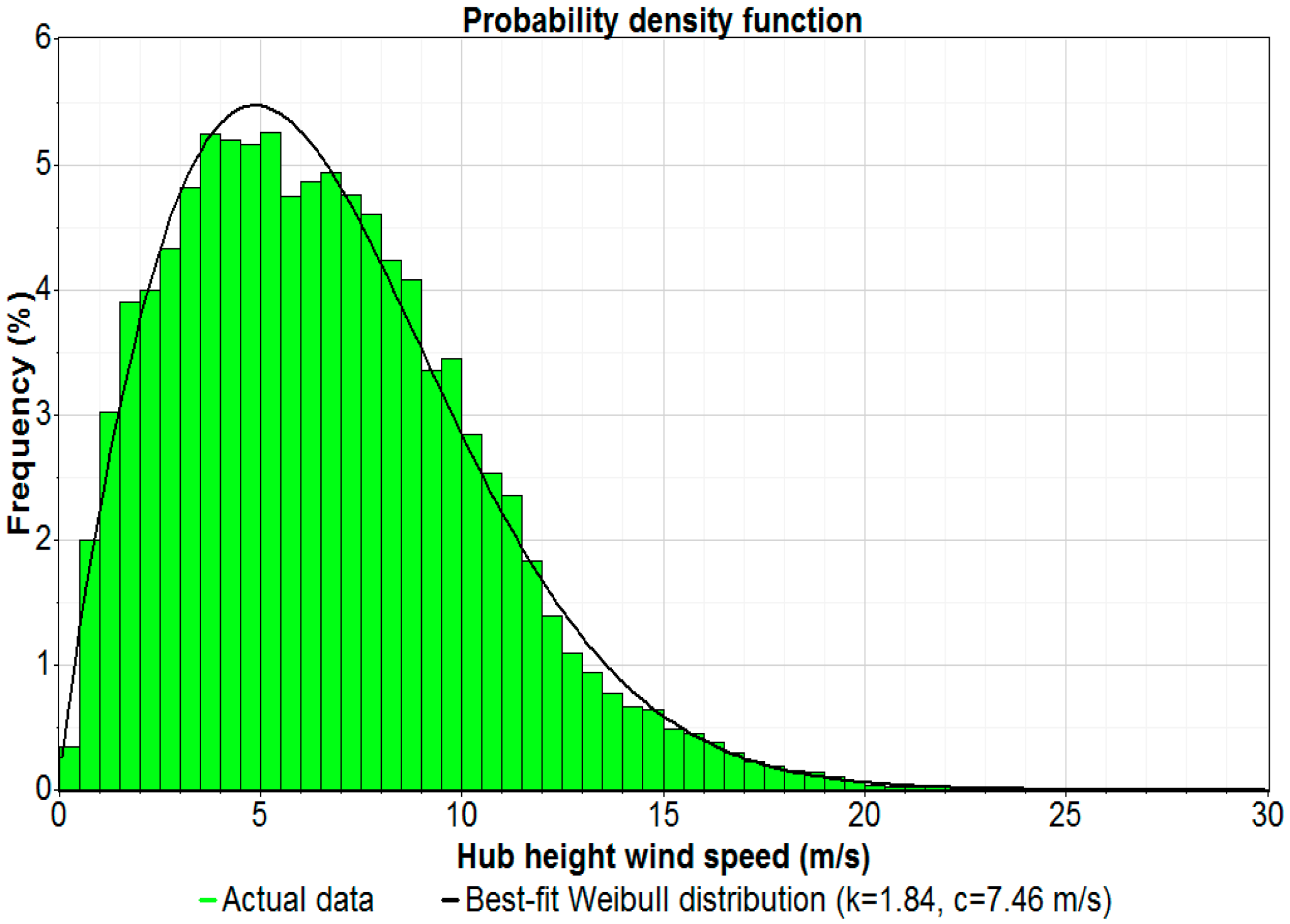
The 12 months’ frequency distribution of wind speed at the hub-height, having a bin size of 0.5 m/s is shown in Figure 5. The wind speed is not uniform and varies to a range of values, and follows Weibull distribution with the parameters k = 1.84 and c = 7.46 m/s. The low values of k imply that the wind speed is not uniform, while the value of c shows the average wind speed at the wind-farm.
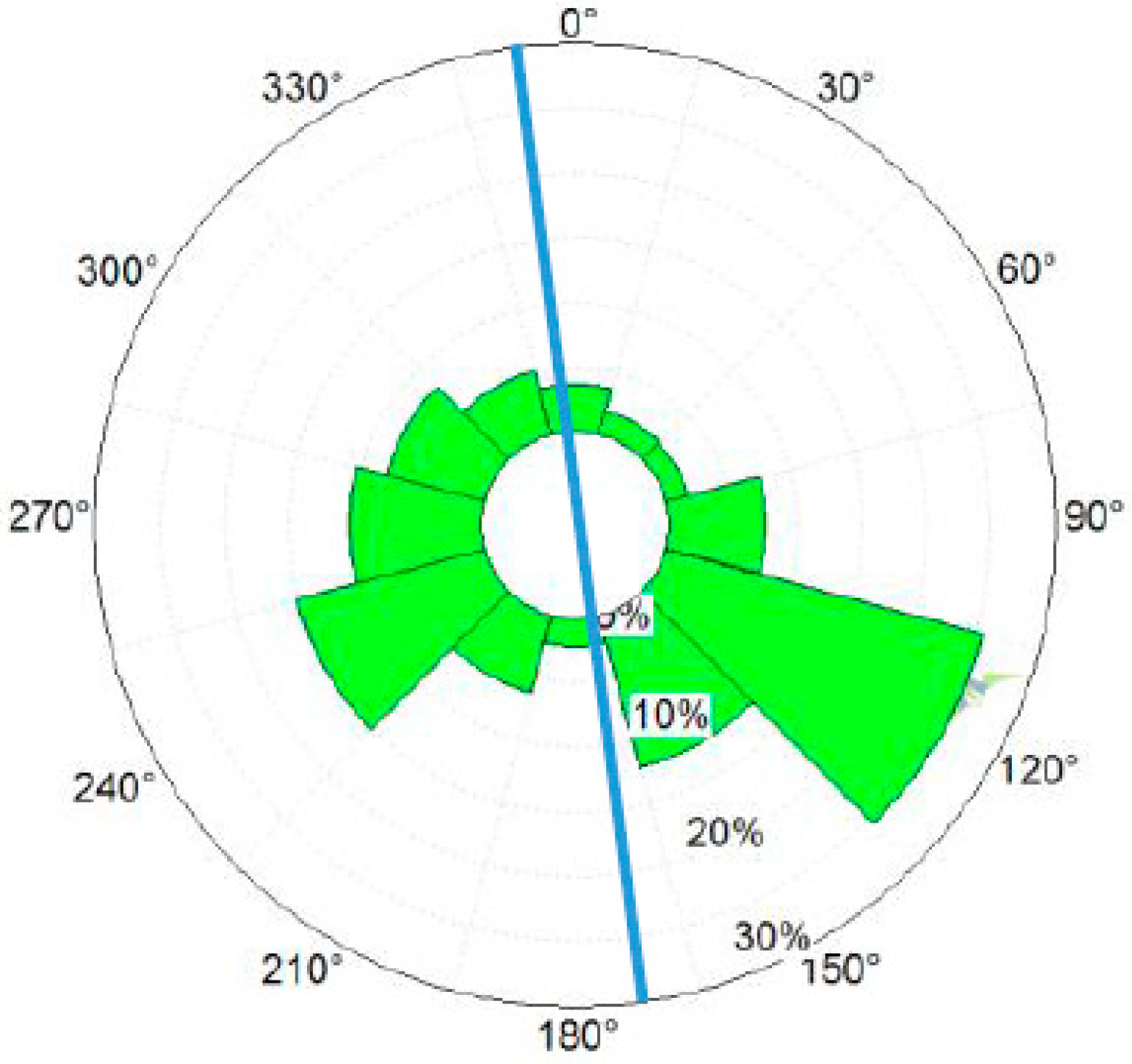
3.2.2. Wind Direction
Wind rose is a graphical tool used to understand the wind direction at any location. It displays the frequency with which wind direction falls in a certain direction sector. The frequency with which the wind blows from a certain direction is shown in Figure 6. As shown, the majority of wind blows from the south-east direction (40%), whereas only 21% of the wind blows from the south-west direction. The power produced by the wind coming from the north is lesser. The blue line shows the position of wind turbines in the wind-farm. Wind turbines are positioned in straight line and make 173° angle with the north.
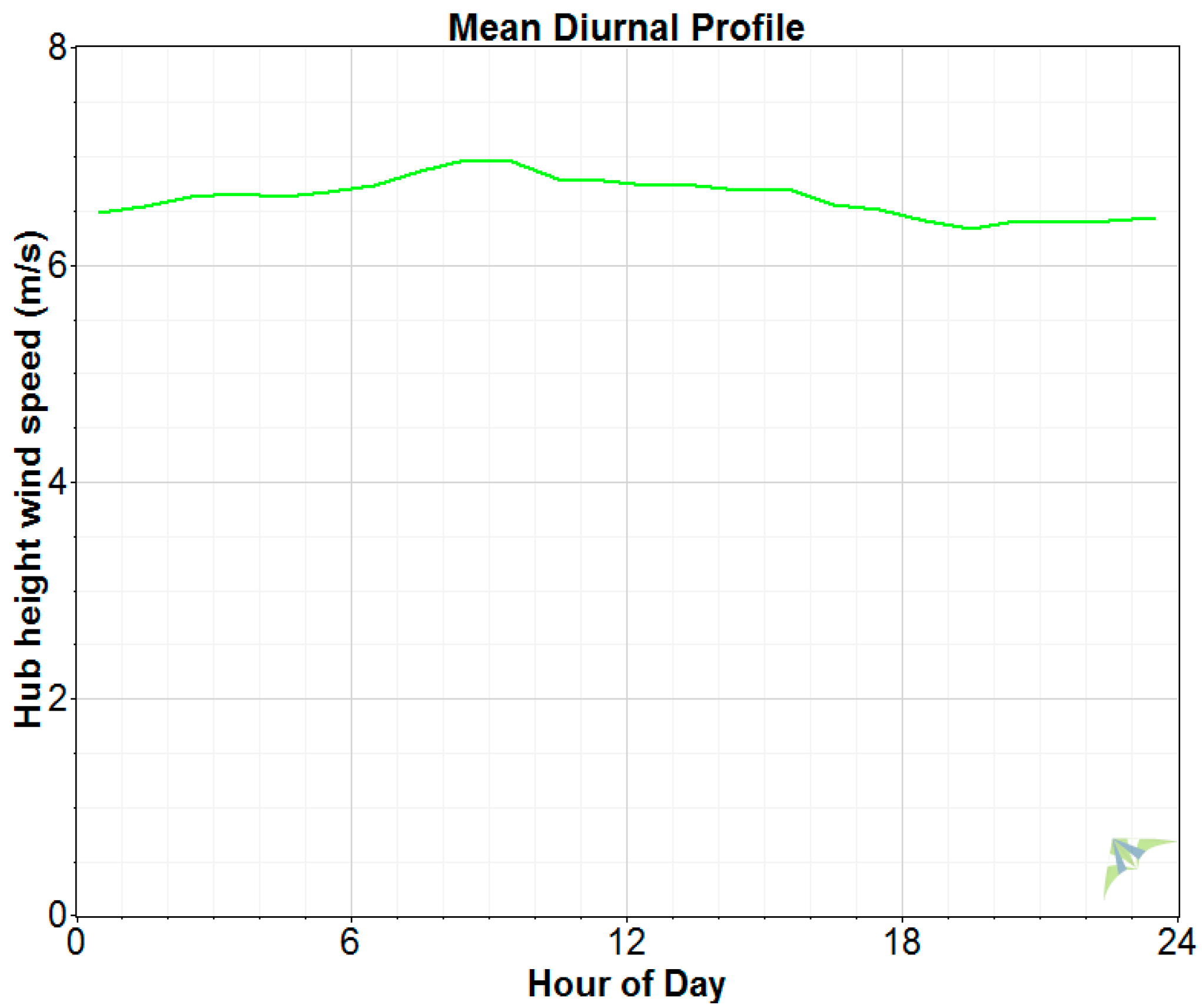
3.2.3. Daily Variation of Wind Speed
The wind speed at a given site does not remain constant throughout the day. The diurnal profile of the wind farm can be obtained to observe the behavior of wind speed over the year. The variation in the wind speed is not too significant throughout the year, however the wind speed is slightly greater in the daytime as compared to the night time (see Figure 7). The average wind speed reaches its maximum at around 9 a.m. and then it reduces and reaches its minimum value at around 8 p.m.
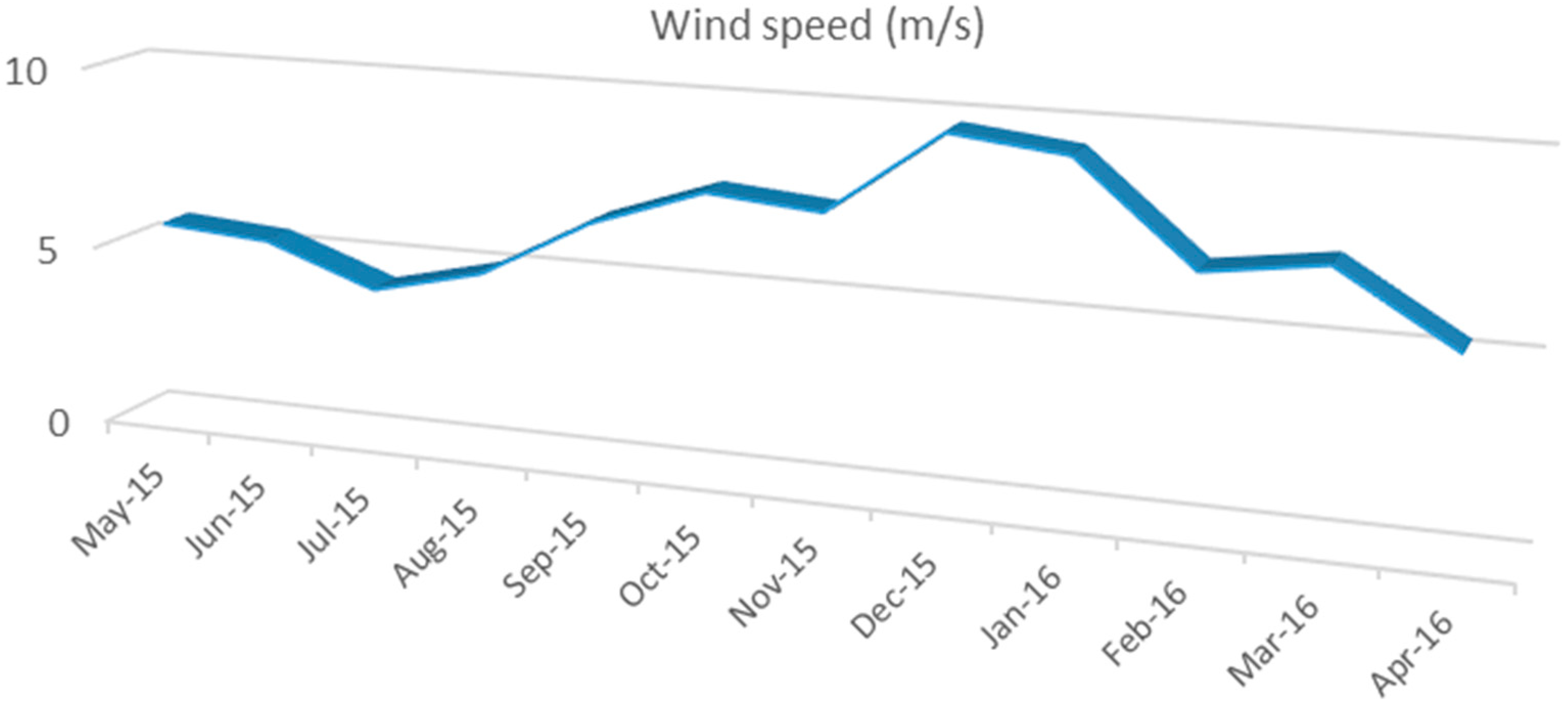
3.2.4. Monthly Wind Speed
The 10-min averaged data from LIDAR was analyzed to obtain mean monthly wind speed profile of the wind farm from May 2015 until April 2016. As observed from Figure 8, the average wind speed was higher in the winter months and reached its maximum level in December (9.70 m/s). However, the summer months had lighter wind, and hence, lower power output was obtained, having the lowest value in July (4.27 m/s). It can further be observed that the wind speed started increasing after July, and decreased after reaching its maximum in December.
3.2.5. Wind Power Class
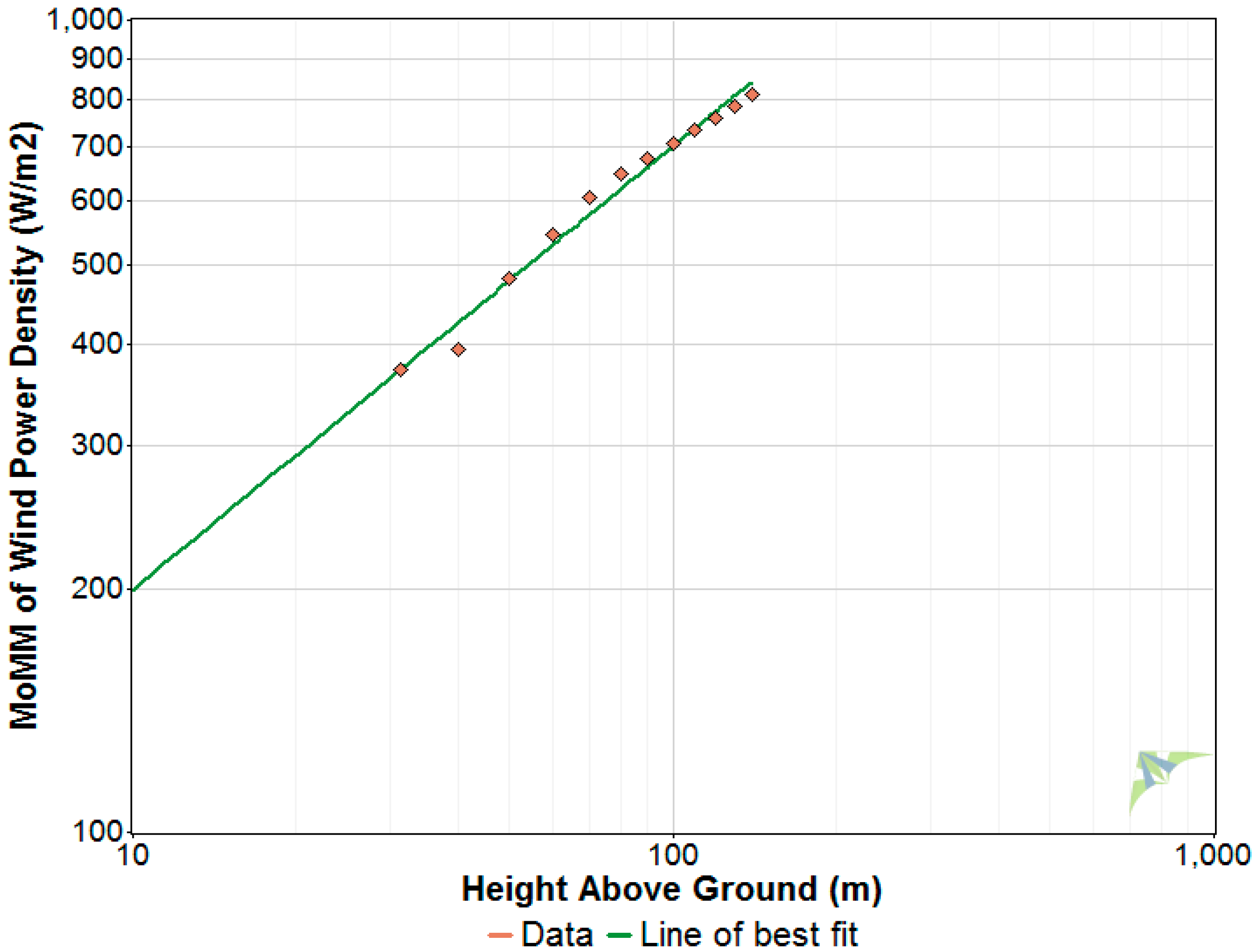
The wind power class is defined as a number showing the energy content at any location. It depends on the mean wind power density at a 50 m height above the ground. Usually, class 3 and above are considered appropriate for the wind power production (see Table 2).
The monthly wind power density (WPD) and Wind Power Class (WPC) of the wind-farm under consideration is given in Table 3. It is observed that the wind farm is suitable for the wind power production, apart from the months of April, June, July, and August when the WPC is less than 3. However other months are rated good for the power production. WPC of 7 was obtained in the months of December and January, which is rated as ‘superb’. Since the WPD varies in the vertical direction, the Linear Least Squares (LLS) regression can be used to obtain the straight line that best fits the natural logarithmic variation of mean wind speed with a natural logarithmic variation of height. To obtain the best estimate of WPD for the whole year, Windographer [13] computes the mean power density at which the best fit line crosses 50 m height. As shown in Figure 9, the mean WPD at 50 m was 479 W/m2 which is wind power class 4. From Table 2, the wind farm falls under ‘good’ and close to ‘excellent’ class for the wind power production.
3.3. Long-Term Analysis
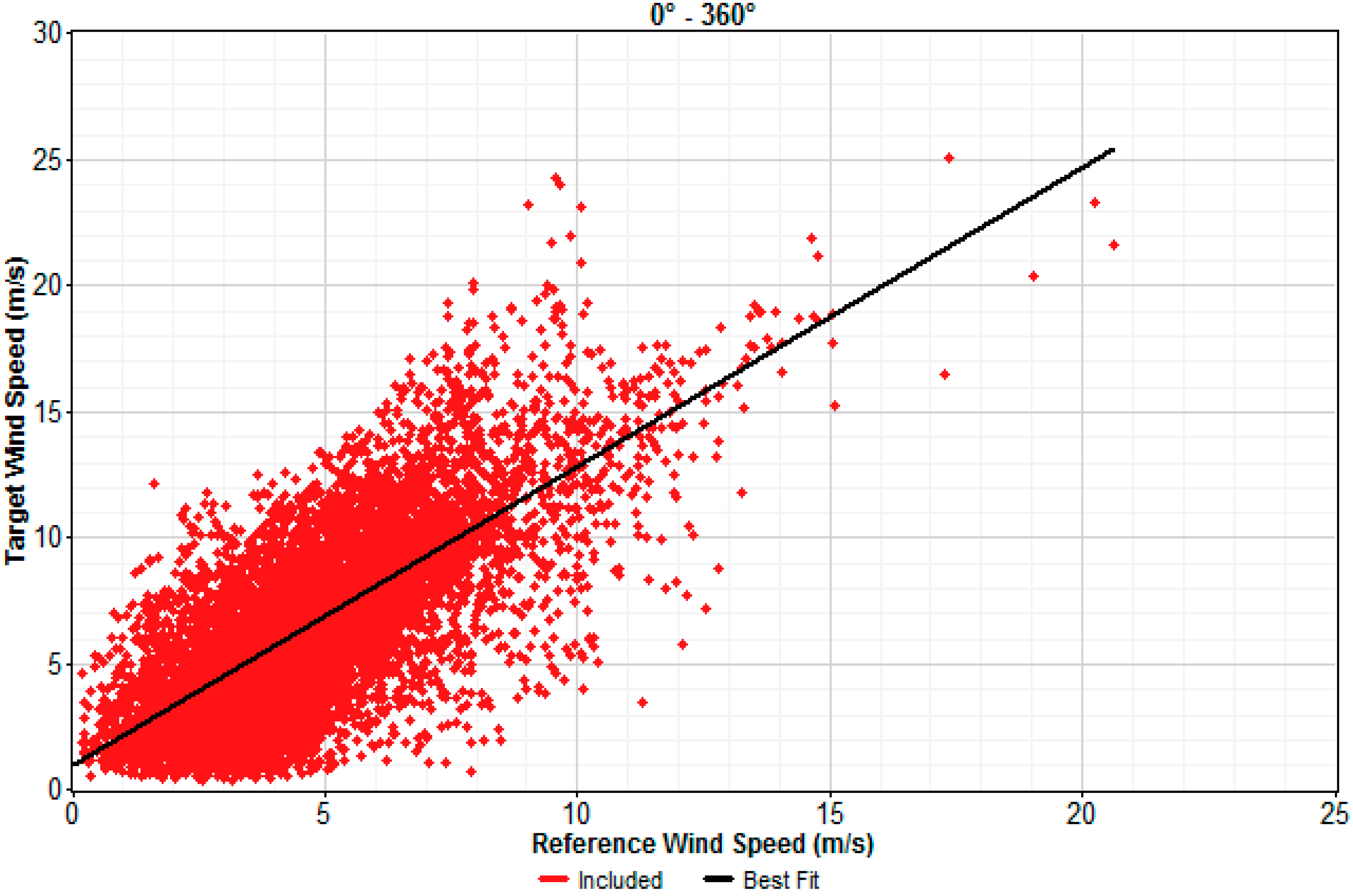
Thus far, the wind resource analysis of 12 months’ period was performed; however, in order to perform a long-term analysis of the wind-farm, there is a need to compare on-site data with the metrological station data. In this study, the Measure-Correlate-Predict (MCP) method is used to evaluate the relationship between the wind data of the target site (wind farm) and the nearby reference station (metrological station having coordinates 63.5 N, 9.375 E).
The MCP feature of Windographer lets the users analyze the relationship between wind speed and direction data measured concurrently at the target location, and a reference location. The data from both stations should have some overlap in time because the Windographer analyzes the correlation in concurrent data. Based on the relationship between the target and reference location, Windographer applies the correlation to synthesize target data (wind speed and wind direction) in time steps that contain reference data but no target data [28]. Moreover, both the target and reference data should have the same time step. Windographer averages or subdivides time steps as needed to generate processed data with the time step of choice. This enables users to have the same target and reference processed data time steps and their time steps perfectly align with each other.
In our case, the 12 months target data is compared with the 38 years reference data having 12 months of concurrent period. The target data with a resolution of 10-min was converted by Windographer to 60-min data, and then compared with the 60-min data of the reference station (Table 4), hence the number of time steps of speeds and direction has reduced after processing the data.
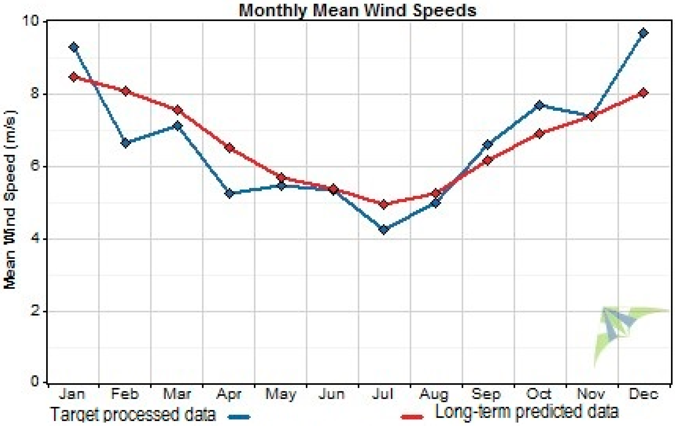
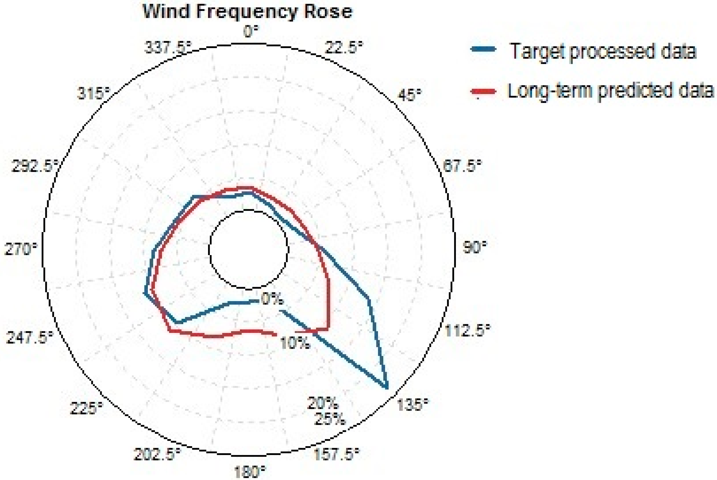
Figure 10 depicts the correlation between the target and reference wind speeds for all the directions using Linear Least Squares regression (LLS) [29]. The value of correlation between the target and reference data is 0.527, which can be classified as a ‘moderate correlation’ according to the rule of thumb stated in [30]. This long-term data of the wind farm is predicted based on the reference data (as explained above), that is shown in Figure 11. It can be established that winter is windier than the summer while December and January have highest wind speeds. The wind direction based on 38 years’ data shows that majority of the wind blows from south-east and south-west directions (see Figure 12).
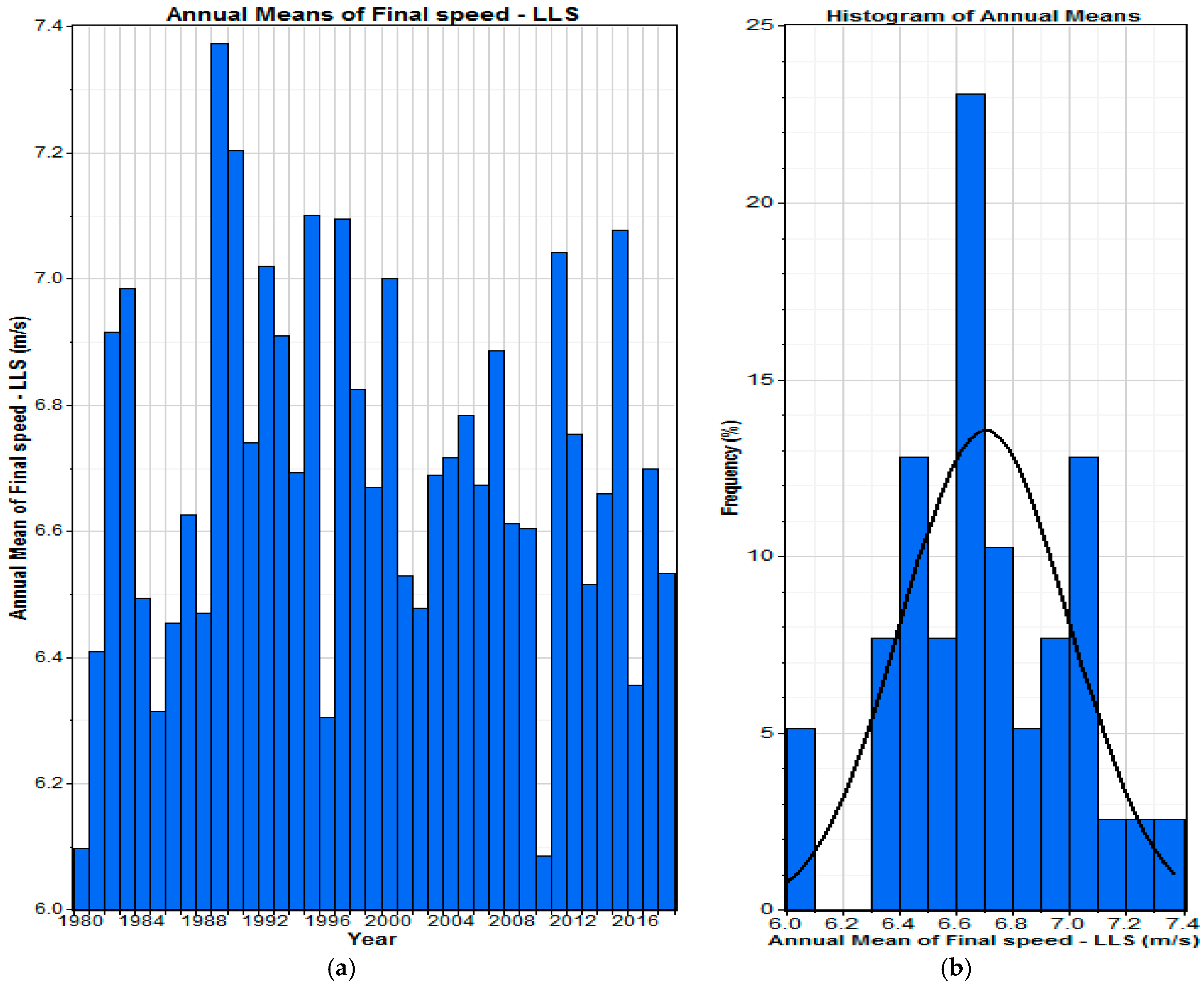
Table 5 compares the target and final predicted data, where final predicted data refers to the long-term predicted data of the wind farm. It can be observed that the long-term mean predicted wind speed of the wind farm is 6.705 m/s, which is about 1% greater than the original mean wind speed. The multi-annual variation of predicted mean wind speed at the wind farm is shown in Figure 13, where LLS shows the results after Least Squares Regression has been performed. The annual mean wind speed of the wind farm varies from 6 m/s to 7.4 m/s.
4. Power Performance
4.1. Theory
The power available in the wind is computed by the ‘method of bins’ based on the IEC61400-12-1 standard. The theoretical maximum efficiency of the wind turbine is 59% (Betz limit). However, efficiency of 30–45% is achieved even for the best-designed wind turbines, when the losses due to gearbox, generator, bearings and wake effects are considered. Power available in the wind can be calculated by [19]:
where, V is the velocity, A is the swept area, is the standard air density, is the power coefficient and is the power available in the wind. The power data is acquired by applying “method of bins” with the bin size of 0.5 m/s, and by calculating the power output and mean values of normalized wind speed in each bin:
where is the normalized/averaged wind speed in bin I, is the normalized wind speed of data set j in bin I, is the normalized/averaged power output in bin I, is the normalized power output of data set j in bin i. is the number of 10-min data sets in bin i. is the power coefficient in each bin.
4.2. Methodology
The wind data from the LIDAR was acquired for 12 months, and the power available in the wind was estimated by Windographer. The actual monthly power produced by the middle wind turbine was noticed for 12 months. Due to the unavailability of power data of other wind turbines, the focus was set on the middle wind turbine, and all the results and comparisons presented in this study are based on the middle wind turbine.
4.3. Results
4.3.1. Mean Power and Energy Output
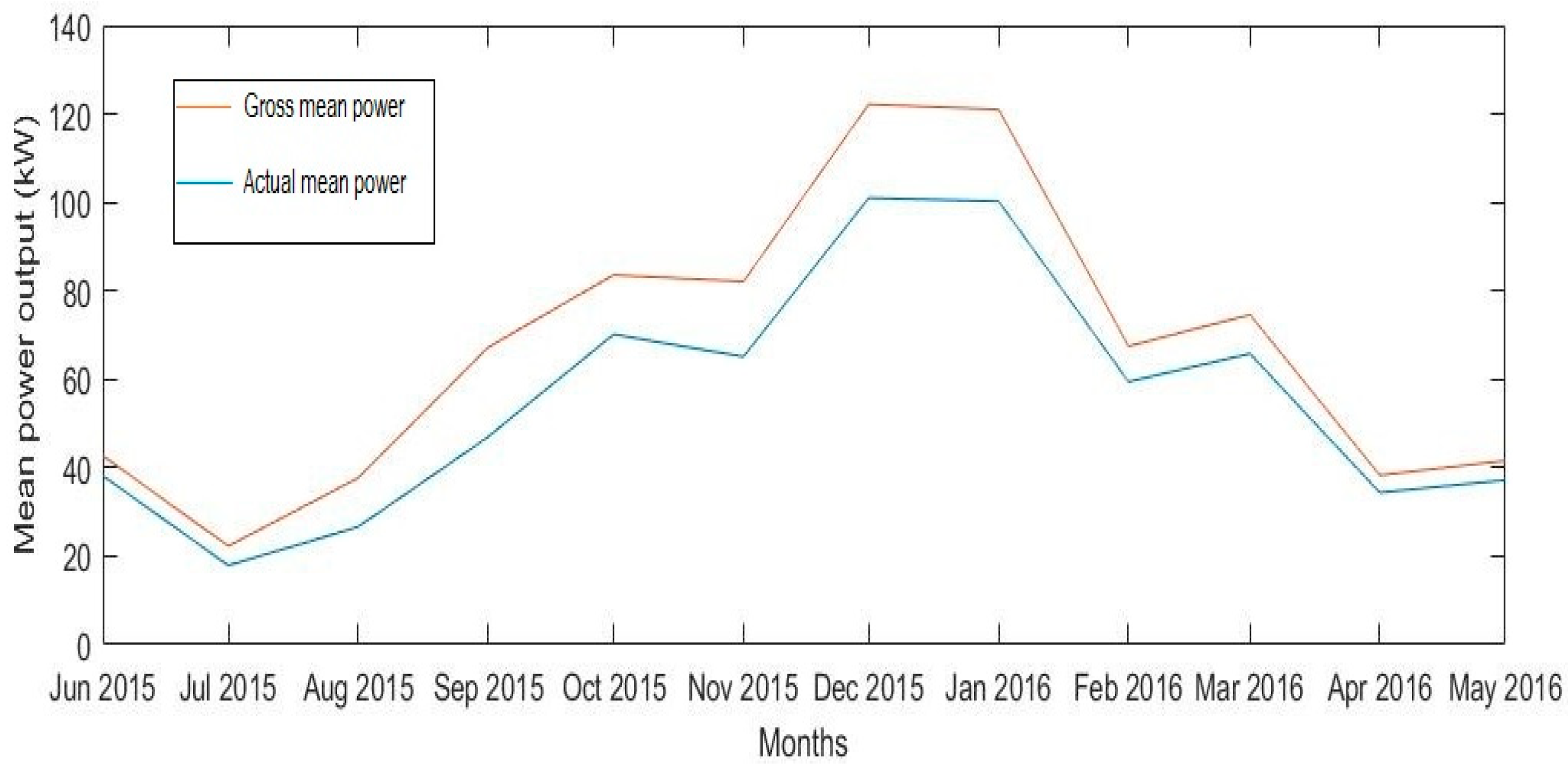
The mean energy and power output data for 12 months are given in Table 6. Gross mean power and energy data is based on the power available in the wind, that wind turbine V-27 should ideally produce based on the power curve data given by the manufacturer (Figure 4). However, the actual mean power and energy data indicates the real power and energy produced by the wind turbine at the site.
The monthly variation of the mean power output is shown in Figure 14. The monthly mean power output of the wind-farm. It can be observed that higher average wind speed results in higher power output during the winter, where maximum power of 101.01 kW and 100.24 kW is produced in December and January respectively. These two months contributes 30% of the annual power production. However, summer months are not ideal for the perspective of power production, and the lowest power produced is 17.92 kW (July).
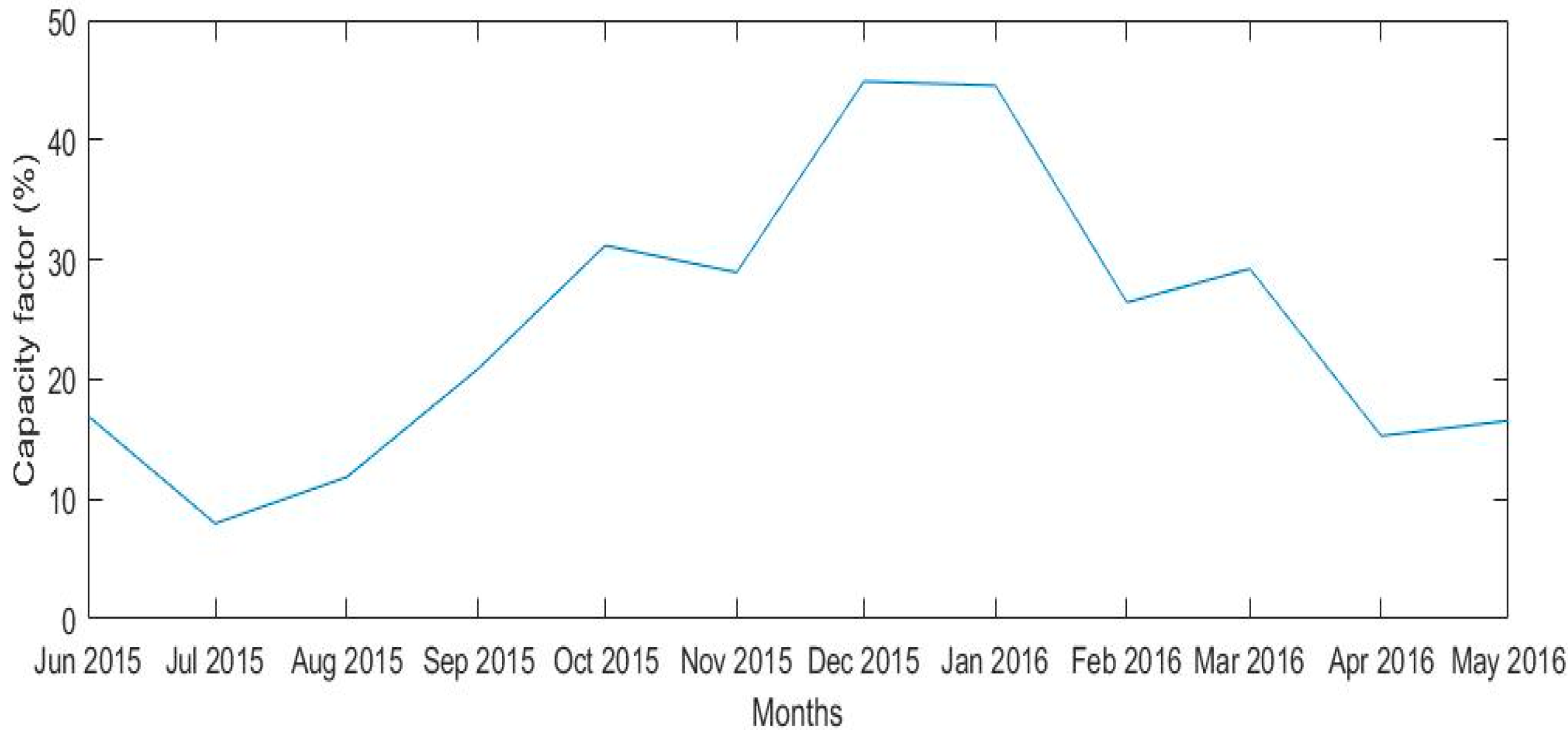
Figure 15 depicts the monthly variation of the capacity factor of the wind farm. The capacity factor of a wind turbine is defined as the actual power produced by a wind turbine compared to the maximum possible power output during that time. It can be observed that the capacity factor is higher in the winter months and reaches the maximum value of around 45% in December and January, while the value is much lower during the summer. The actual capacity factor of the wind turbine over the year is 24.55%, while the gross capacity factor estimated by Windographer based on the wind resource for V-27 is 29.95%. It can be concluded from this observation that the overall losses of the wind turbine are around 18%. These losses are the combination of wake effects, bearing losses, availability losses, and generator losses. The overall capacity factor of 24.55% for the wind turbine is a good number in the European context because the average capacity factors in Europe, Germany, UK, Netherlands, and France from 2003–2007 were 20.1%, 29.3%, 25.9%, 25.7% and 21.8%, respectively [31].
4.3.2. Histogram of Gross Power
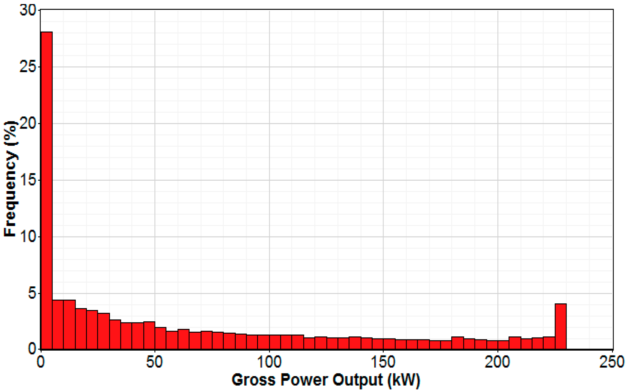
The histogram of gross power, shown in Figure 16, represents the frequency of distribution of gross power produced by V-27 and is based on the wind speed measurements of LIDAR. The wind turbine has produced its rated maximum power (i.e., 225 kW) only 4% of the times, whereas less than 5 kW power was produced 28% of the times.
4.3.3. Power Curve
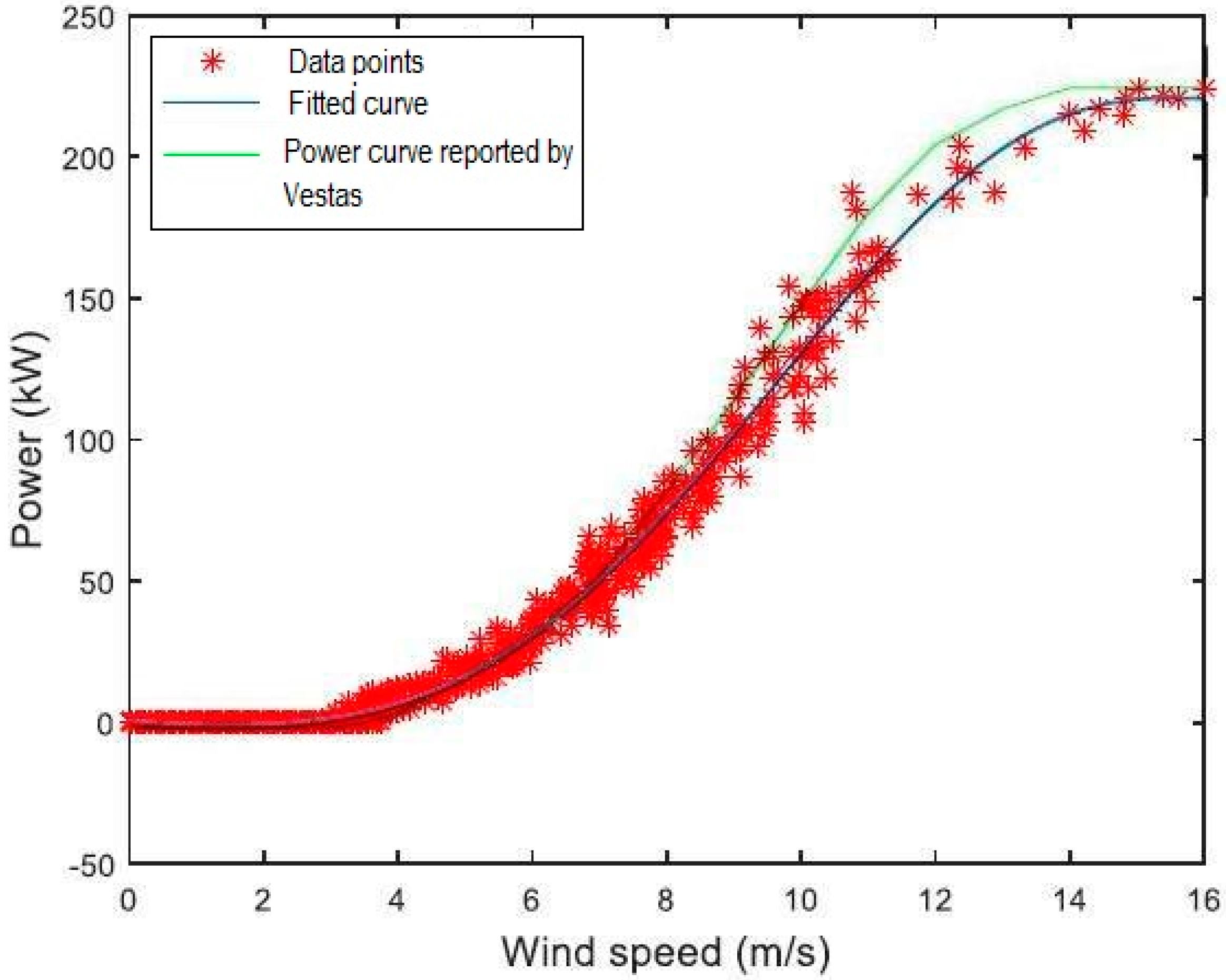
The performance of a wind turbine is generalized by its power curve. The power output of the middle wind turbine was observed for 2 months. The wind speed and power data of the wind turbine are used to obtain the scatter plot. The best fit curve on the data points was plotted using polynomial curve fitting in the MATLAB R2018b by MathWorks Inc. The polynomials of various orders were tested to fine tune the coefficients to the data points. The polynomial curve fit of 8th order is plotted in Figure 17. As can be seen, a good fit with the data was found.
Moreover, Figure 17 compares the power curve of the wind turbine V-27 at the wind farm obtained with a best fit curve, and the power curve reported by the manufacturer (Figure 4). It is observed that the power curve of V-27 matches almost precisely with the manufacturer’s power curve up to the wind speed of 7 m/s. However, the gap widens and reaches its maximum level (almost 16%) at 11.80 m/s. This deviation is not only caused by the losses but also due to the unavailability of enough data above the wind speed of 10 m/s.
5. Revenue Estimation
5.1. Electricity Market in Norway
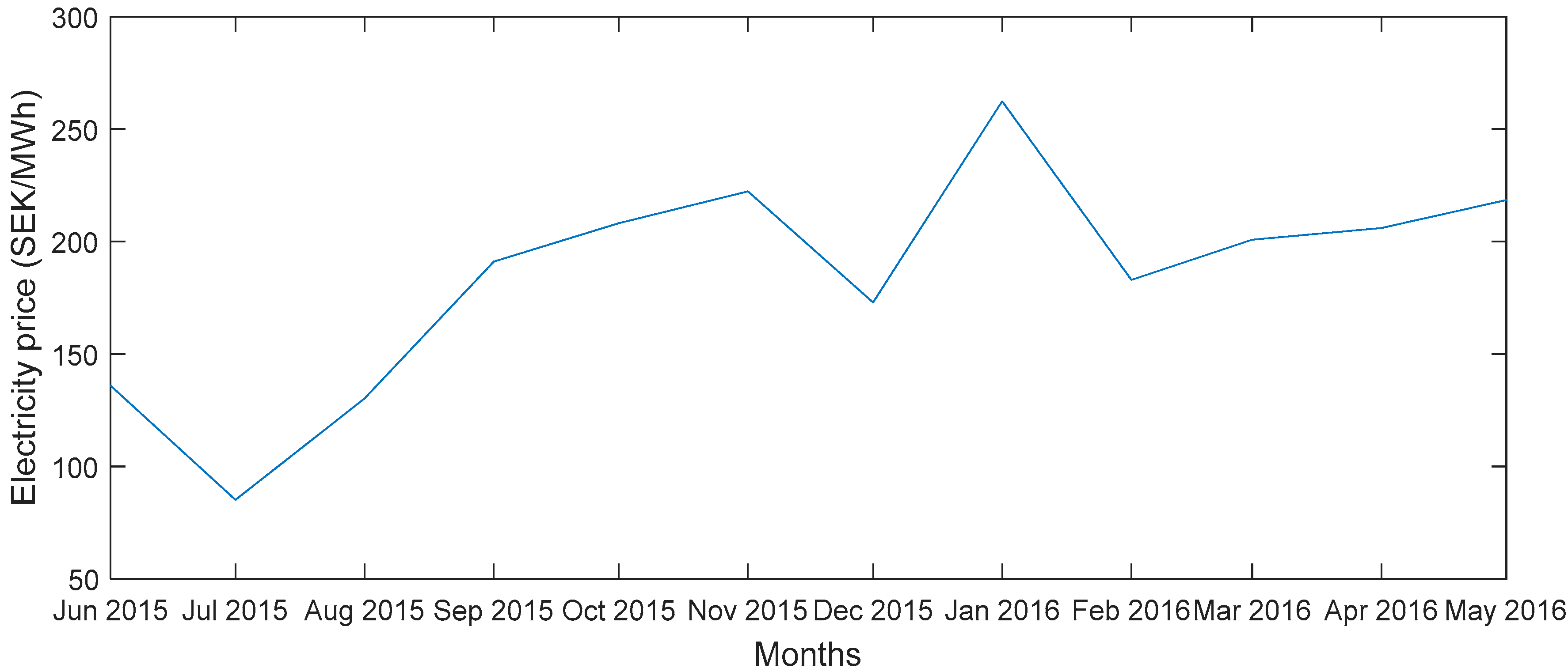
The Energy Act, which manages the production, conversion, transmission, trading, distribution, and use of energy in Norway, follows market-based power trading. Norway is embodied in the joint Nordic Power market along with Sweden, Finland and Baltic countries, where most of the generated power is traded on Nord Pool spot power exchange based on market demand [32]. In addition to the market demand, the price also depends on the variation of climatic conditions, economic growth and electricity exchange between the participating countries of the Nordic power market [33]. The variation of monthly average spot prices for the location is shown in Figure 18. It can be seen that the prices have sharply increased after 15 July and reached the highest level in 15 January.
In order to achieve the country’s goals under the EU’s Renewable Energy Directive, Norway and Sweden have established a joint Norwegian-Swedish tradable green certificate (TGC) since 2012 [35]. TGCs are financed by the consumers, and the producers of renewable energy have the right to sell each certificate. However, unlike feed-in-tariff, both TGC prices and electricity prices are high in winter and low in summer. That means TGC also varies in price according to the principle of supply and demand.
According to Norwegian Energy Certificate System (NECS) [36] and Cesar [37], approximately 58.7 million electricity certificates were sold during the period 1 April 2015 to 31 March 2016, which showed an increase of 62 percent compared to same period one year earlier. This includes spot trading during the year, forward contracts with the physical transfer of certificates during the period and transactions within the same group of companies [38].
Since TGC and electricity prices are tied up, unlike systems that support a certain amount such as feed-in tariff, the monthly revenues of new renewable energy producers will not always be proportional to wind speed or wind direction. Comparing the graph in Figure 19 with the graph shown in Figure 18, it is seen that the highest power was produced during December 2015 whereas the greatest income was produced during January 2016.
5.2. Monthly Income Stream
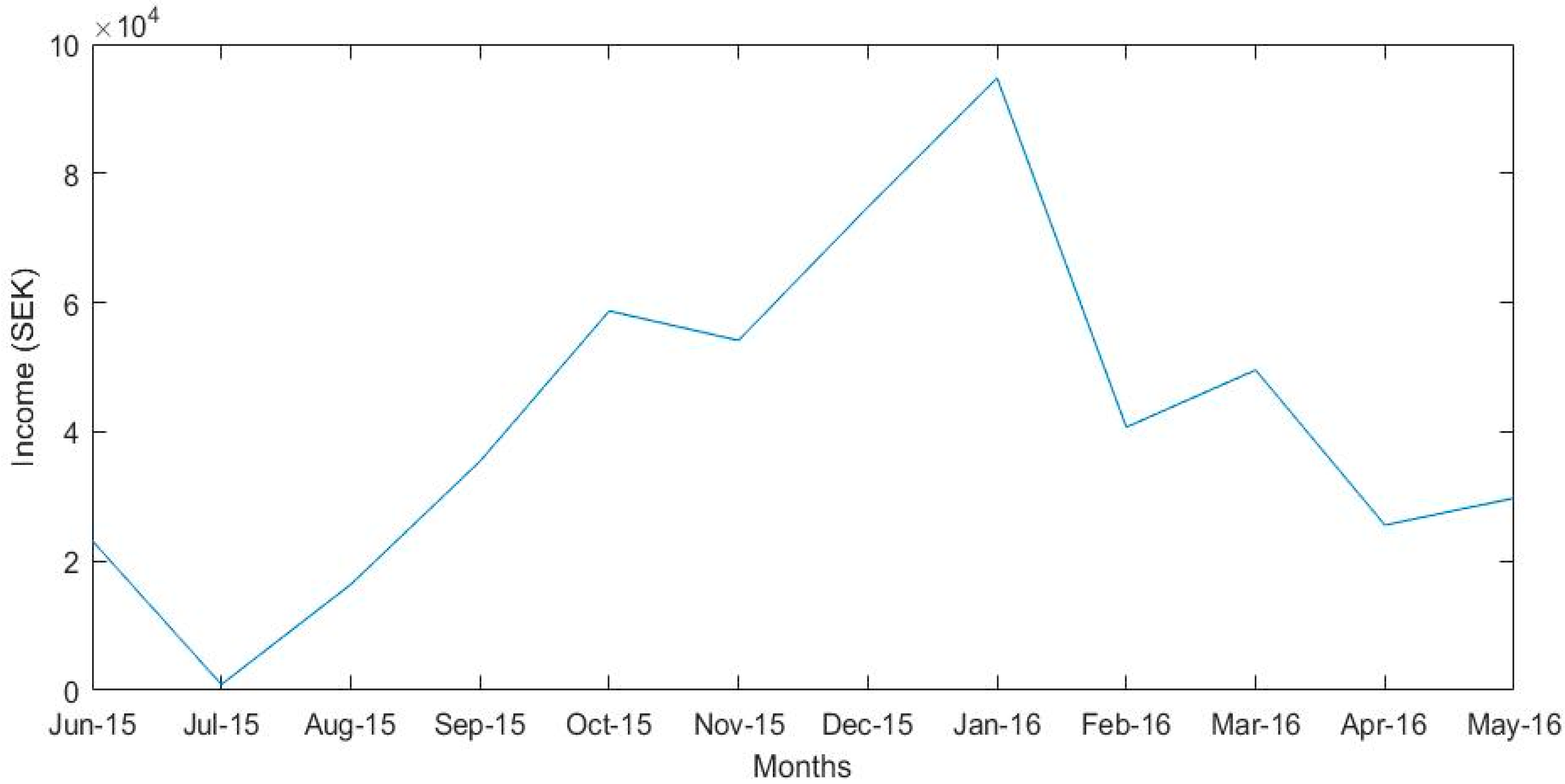
This study estimates the income stream of the wind farm based on average monthly spot prices of electricity on the Nord Pool power exchange as well as average monthly prices of TGCs. The figures are based on the actual monthly mean energy output of the middle wind turbine, and it is assumed that the output of the other two wind turbines is equal to the middle wind turbine. The monthly income stream from the wind farm is depicted in Figure 20.
The minimum income of the wind farm was estimated to be 9004.8 SEK which was generated in July because of the lowest mean wind speed (4.27 m/s) and the lowest electricity price (85.11 SEK/MWh). However, the maximum estimated income from the wind farm was 93,603.6 SEK which occurred in the month of January, when a total of 223.7 MWh electricity was generated from the wind farm. The income in December (74,773.5 SEK) was lower than the income in January, despite the fact that more energy was produced in December (225.4 MWh). This pattern shows the high dependence of income on the spot prices of electricity and the tradable green certificates, while the wind speed at a site certainly has an impact on the overall production of the wind farm.
The estimated annual energy production (AEP) of the wind farm is 1450.6 MWh/year. The annual estimated income of the wind farm under consideration is obtained by the summation of monthly incomes, which will equal 508,004 SEK.
5.3. Simulation Wind-Farm’s Income
The effect of market-based electricity prices and TGC prices on the income of wind farm was discussed in the above section, but the statistical nature of electricity prices and TGC prices were not considered. For this purpose, the MCS approach is used to estimate the wind farm’s income and to investigate the effect of price components on the mean income by conducting sensitivity analysis. Ten years historical data of the electricity prices and TGC prices was obtained to derive the monthly values of mean and standard deviation of both parameters (see Table 7). The @Risk software [40] was used for 10,000 iterations of MCS of each month, where both input parameters were assumed to follow a normal distribution. The MCS derived the PDFs of monthly incomes by generating random values of monthly electricity prices and TGC prices (based on the parameters as given in Table 7). These PDFs were further used to obtain the simulated monthly mean incomes, shown in Figure 21. It was eventually found that both the simulated and actual incomes of wind farm follow an identical pattern. The generated income is much higher in the winter months than summer months. However, an interesting observation was that the simulated income values were higher than the actual income (of 2015–2016), which shows the prices have been declining over the years (historical mean prices are higher than actual prices in 2015–2016).
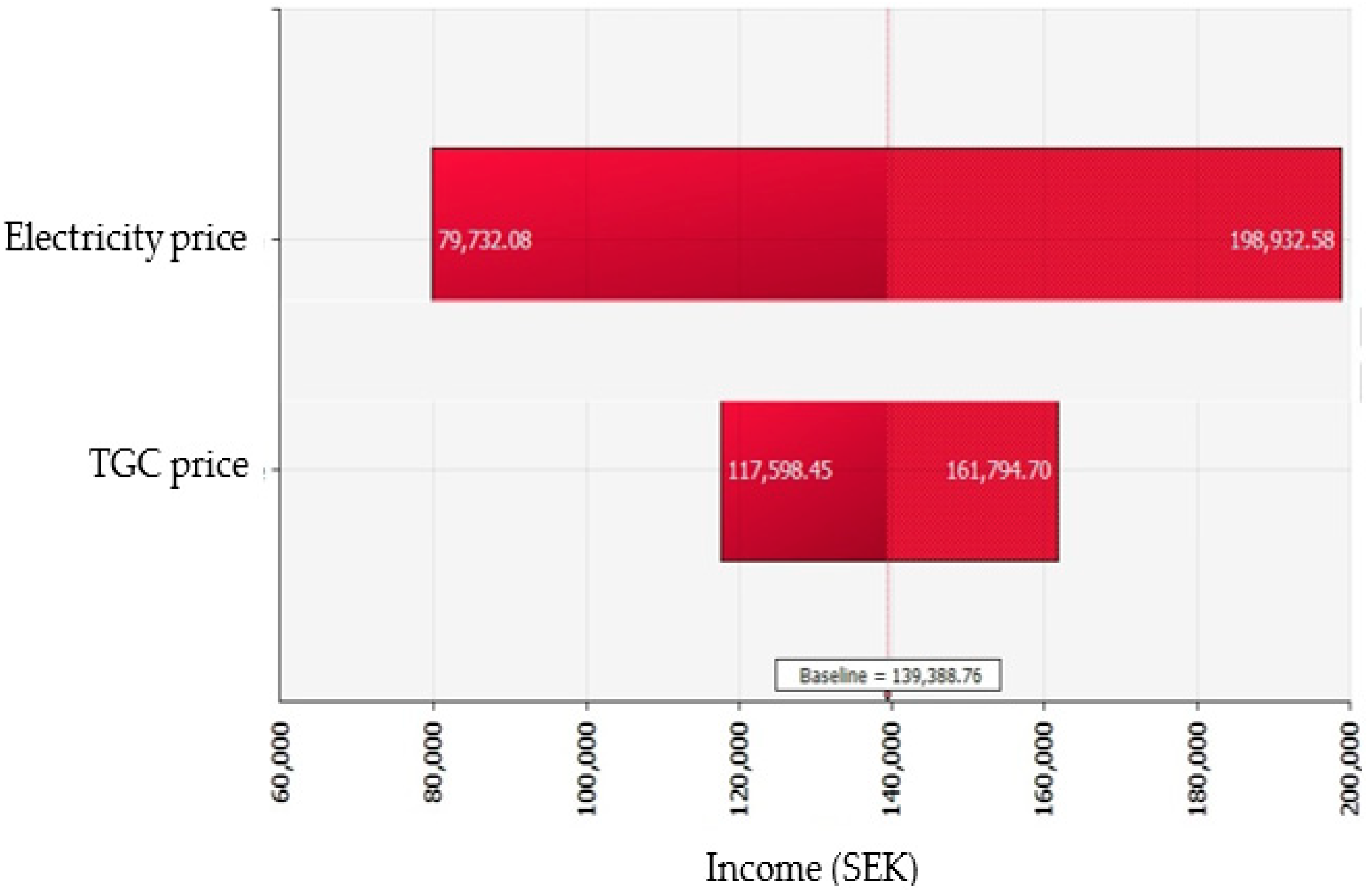
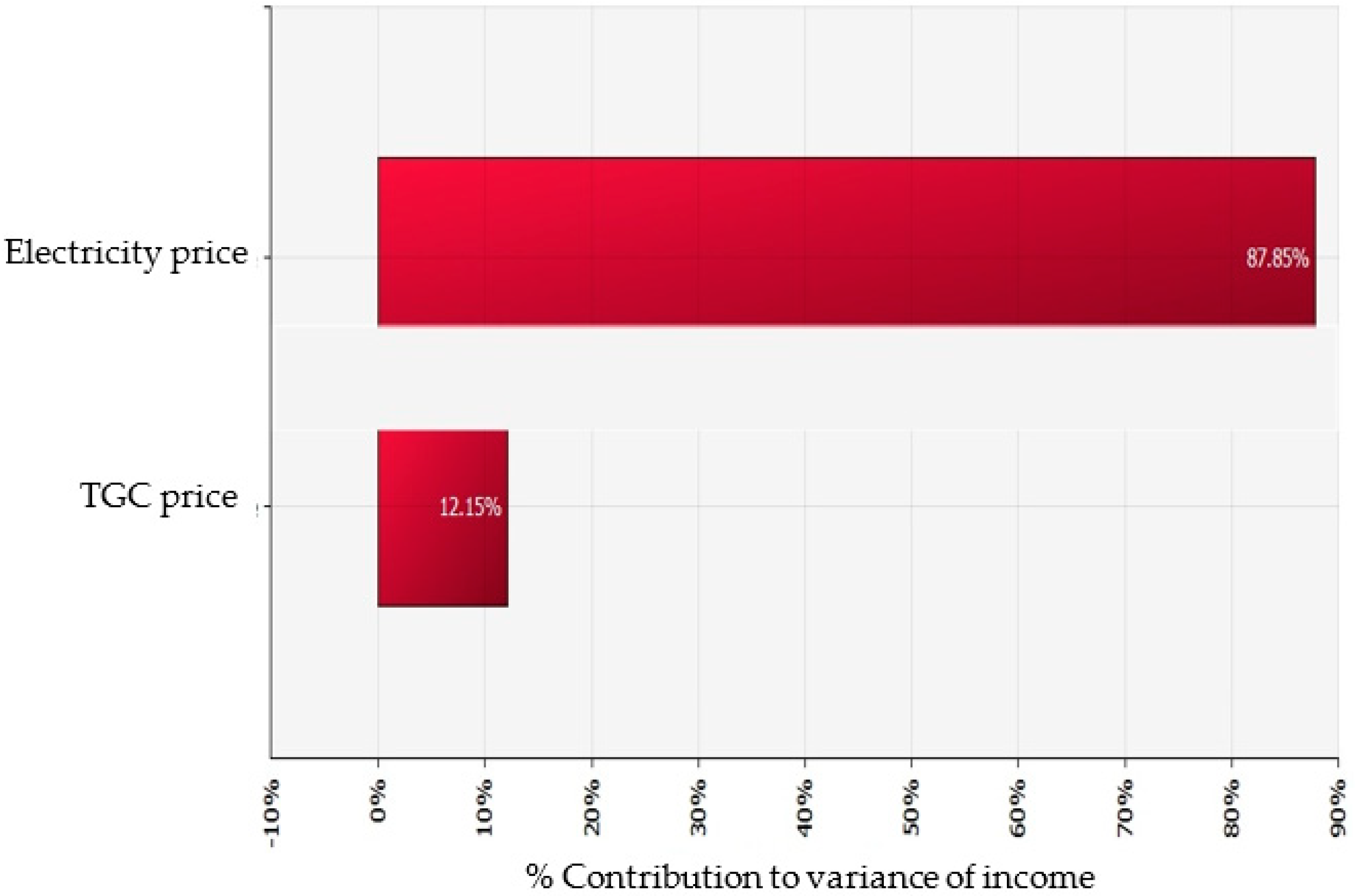
Moreover, the sensitivity analysis was performed using @Risk software to see how both the prices affect the overall monthly incomes. For the sake of demonstration, a ‘Tornado graph’ for the month of January 2016 is represented in Figure 22. Tornado graph shows how the simulated income of the wind farm varies as each uncertain price varies over its range. The input at the top has the highest impact on the income of wind farm. Also, Figure 23 shows the contribution of each input to the variance of mean monthly income for January. The contribution of electricity prices to the variance of monthly income for January 2016 is 87.85%. While the contribution of TGC prices to the variance of income for January 2016 is 12.15%. This implies that electricity prices have a much higher impact on the monthly income of wind-farm compared to the TGC prices.
6. Conclusions and Future Work
In this study, a wind resource analysis on a wind farm comprising of three wind turbines was performed using the wind turbine IEC61400-12-1 power measurement standard and the 12 months data collected from the LIDAR located at the wind farm. For the long-term analysis, MCP method was used to predict wind behavior by comparing it with the 38 years’ wind data collected from a metrological station located at 63.5 N, 9.375 E. It was observed that winter season contributed considerably towards the AEP, where only the months of December and January contributed to 30% of the AEP. Moreover, it was found out that wind mostly comes from south-east and south-west directions at the wind farm. Wind power class of the wind farm was also rated between 4 and 5, which represents good to excellent category.
Mean monthly power and energy output of a Vestas V-27 wind turbine was obtained and was further compared with actual power production of the wind turbine. It was observed that the power production calculated based on the power curve provided by the manufacturer was greater than the actual power produced, due to wake effects losses, bearing losses, availability losses and generator losses. The power curve acquired by the best fit curve of the measured data in the wind farm showed a similar trend as the actual power curve.
The effect of spot prices of electricity and the TGC on the income generated by the wind farm was also investigated. The income generated by the wind farms in Norway depends heavily on the principle of demand and supply. The TGC market gives incentives to the producers of renewable energy by issuing a certificate for each MWh of energy produced. However, the income may significantly be affected once the TGC market seizes to operate after 2035. It was observed that the impact of electricity prices on the income of wind farm is much higher than the effect of TGC prices. The percentage contribution of electricity price and TGC price to the variance of monthly income for January is 87.85% and 12.15% respectively. Moreover, a similar pattern was observed for other months. It can be concluded that the variation in TGC prices over the years has been outnumbered by the variation in electricity prices. Although, TGC prices have a significant contribution to the overall income, their contribution to the income has remained fairly consistent over the years.
Further work should be performed by mounting a data logger to get accurate time-series of the wind turbine, which will further enhance the accuracy of the power curve. The power output data of other two wind turbines could also be observed to study the effect of wake on the wind farm’s performance. The initial investment cost, Operation and Maintenance (O&M) costs, and other costs data should be obtained to calculate the Levelized Cost of Energy (LCoE), Net Present Value (NPV) and Internal Rate of Return (IRR) to measure the financial performance of the wind farm [41,42].
Author Contributions
A.M. performed the analysis and wrote the manuscript text. M.S. reviewed the manuscript and made contributions to its structure.
Funding
This work was supported by the UK Engineering and Physical Sciences Research Council (EPSRC) grant EP/L016303/1 for Doctoral Training in Renewable Energy Marine Structures (REMS).
Acknowledgments
The author would like to acknowledge the Norwegian University of Science and Technology (NTNU) and Lars Roar Sætran for providing support in carrying out the work and installing LIDAR on the wind farm.
Conflicts of Interest
The authors declare no conflict of interest.
Nomenclature
| MCS | Monte-Carlo Simulation |
| EU | European Union |
| LIDAR | Laser Imaging Detection and Ranging |
| SODAR | Sonic Detection and Ranging |
| MCP | Measure-Correlate-Predict |
| TGC | Tradable Energy Certificate |
| Probability Density Function | |
| ML | Maximum Likelihood |
| WPC | Wind Power Class |
| WPD | Wind Power Density |
| k | Weibull shape factor |
| c | Weibull scale factor |
| LLS | Linear Least Squares |
| MoMM | Mean of Monthly Means |
| CP | Power coefficient |
| Pavail | Power available in the wind |
| SEK | Swedish Krona |
| AEP | Annual Energy Production |
References
- Presencia, C.E.; Shafiee, M. Risk Analysis of Maintenance Ship Collisions with Offshore Wind Turbines. Int. J. Sustain. Energy 2018, 231. [Google Scholar] [CrossRef]
- WindEurope. Wind Energy in Europe: Outlook to 2020. Available online: https://windeurope.org/about-wind/reports/wind-energy-in-europe-outlook-to-2020/ (accessed on 30 September 2018).
- WindEurope. Wind in Power 2017. Available online: https://windeurope.org/wp-content/uploads/files/about-wind/statistics/WindEurope-Annual-Statistics-2017.pdf (accessed on 30 September 2018).
- Zheng, C.; Xiao, Z.; Peng, Y.; Li, C.; Du, Z. Rezoning Global Offshore Wind Energy Resources. Renew. Energy 2018, 129, 1–11. [Google Scholar] [CrossRef]
- Onea, F.; Rusu, E. Efficiency Assessments for Some State of the Art Wind Turbines in the Coastal Environments of the Black and the Caspian Seas. Energy Explor. Exploit. 2016, 34, 217–234. [Google Scholar] [CrossRef]
- Manwell, J.F.; McGowan, J.G.; Rogers, A.L. Wind Energy Explained: Theory, Design and Application; Wiley: New York, NY, USA, 2009; ISBN 0471499722. [Google Scholar]
- Morten, L.; Saetran, L.R.; Wangsness, E. ScienceDirect Performance Test of a 3 MW Wind Turbine-Effects of Shear and Turbulence. Energy Procedia 2015, 80, 83–91. [Google Scholar]
- Ahmed, A.S. Wind Resource Assessment and Economics of Electric Generation at Four Locations in Sinai Peninsula, Egypt. J. Clean. Prod. 2018, 183, 1170–1183. [Google Scholar] [CrossRef]
- Khan, K.S.; Tariq, M. Wind Resource Assessment Using SODAR and Meteorological Mast – A Case Study of Pakistan. Renew. Sustain. Energy Rev. 2018, 81, 2443–2449. [Google Scholar] [CrossRef]
- Smith, D.A.; Harris, M.; Coffey, A.S.; Mikkelsen, T.; Jørgensen, H.E.; Mann, J.; Danielian, R. Wind Lidar Evaluation at the Danish Wind Test Site in Høvsøre. Wind Energy 2006, 9, 87–93. [Google Scholar] [CrossRef]
- Mifsud, M.D.; Sant, T.; Farrugia, R.N. Comparison of Measure-Correlate-Predict Methodologies Using LiDAR as a Candidate Site Measurement Device for the Mediterranean Island of Malta. Renew. Energy 2018, 127, 947–959. [Google Scholar] [CrossRef]
- Fazelpour, F.; Markarian, E.; Soltani, N. Wind Energy Potential and Economic Assessment of Four Locations in Sistan and Balouchestan Province in Iran. Renew. Energy 2017, 109, 646–667. [Google Scholar] [CrossRef]
- Windographer, Version 4, UL, Albany, NY, USA. Available online: https://www.windographer.com/ (accessed on 30 September 2018).
- Gleim, A.; Keck, R.-E.; Lund, J.A. Monte Carlo Methods to Include the Effect of Asymmetrical Uncertainty Sources in Wind Farm Yield Assessment. Wind Eng. 2018. [Google Scholar] [CrossRef]
- Hrafnkelsson, B.; Oddsson, G.; Unnthorsson, R. A Method for Estimating Annual Energy Production Using Monte Carlo Wind Speed Simulation. Energies 2016, 9, 286. [Google Scholar] [CrossRef]
- Hustveit, M.; Frogner, J.S.; Fleten, S.-E. Tradable Green Certificates for Renewable Support: The Role of Expectations and Uncertainty. Energy 2017, 141, 1717–1727. [Google Scholar] [CrossRef]
- Bai, W.; Lee, D.; Lee, K.; Bai, W.; Lee, D.; Lee, K.Y. Stochastic Dynamic AC Optimal Power Flow Based on a Multivariate Short-Term Wind Power Scenario Forecasting Model. Energies 2017, 10, 2138. [Google Scholar] [CrossRef]
- Aune, F.R.; Dalen, H.M.; Hagem, C. Implementing the EU Renewable Target through Green Certificate Markets. Energy Econ. 2012, 34, 992–1000. [Google Scholar] [CrossRef]
- IEC. IEC 61400-12-1 Wind Turbines—Part 12-1: Power Performance Measurements of Electricity Producing Wind Turbines; IEC: Geneva, Switzerland, 2017. [Google Scholar]
- Marjan, A. Wind Farm Performance; Norwegian University of Science and Technology: Trondheim, Norway, 2016. [Google Scholar]
- Green Energy Wind. Available online: http://www.greenenergywind.co.uk/ (accessed on 30 September 2018).
- Petersen, M. Wind Turbine Test Vestas V27-225 KW; Technical University of Denmark: Lyngby, Denmark, 1990. [Google Scholar]
- Manwell, J.F.; McGowan, J.G.; Rogers, A.L. Wind Energy Explained; John Wiley & Sons, Ltd.: Chichester, UK, 2002; ISBN 9780470015001. [Google Scholar]
- Finkelstein, M.; Shafiee, M. Preventive Maintenance for Systems with Repairable Minor Failures. J. Risk Reliab. 2017, 231, 101–108. [Google Scholar] [CrossRef]
- Canadillas, B. Testing the Performance of a Ground-Based Wind LiDAR System One Year Intercomparison at the Offshore Platform FINO1. Wilhelmshaven. Available online: www.dewi.de/dewi_res/fileadmin/pdf/publications/Magazin_38/08.pdf (accessed on 30 September 2018).
- Şen, Z.; Altunkaynak, A.; Erdik, T. Wind Velocity Vertical Extrapolation by Extended Power Law. Adv. Meteorol. 2012, 2012, 178623. [Google Scholar] [CrossRef]
- NRC. Wind Power Class. Available online: https://www.nrc.gov/docs/ML0720/ML072040340.pdf (accessed on 30 September 2018).
- Øistad, I.S. Site Analysis of the Titran Met-Masts; Norwegian University of Science and Technology: Trondheim, Norway, 2014. [Google Scholar]
- NIST. e-Handbook of Statistical Methods. Available online: http://www.itl.nist.gov/div898/handbook/ (accessed on 30 September 2018).
- Mukaka, M.M. Statistics Corner: A Guide to Appropriate Use of Correlation Coefficient in Medical Research. Malawi Med. J. 2012, 24, 69–71. [Google Scholar] [PubMed]
- Boccard, N. Capacity Factor of Wind Power Realized Values vs. Estimates. Energy Policy 2009, 37, 2679–2688. [Google Scholar] [CrossRef]
- Breitschopf, B. Electricity Costs of Energy-Intensive Industries in Norway—A Comparison with Energy-Intensive Industries in Selected Countries. Available online: https://www.energinorge.no/contentassets/525e77b1feff4203a94ef6d1f94cfd03/electricity-costs-ofenergy-intensive-industries-in-norway.pdf (accessed on 30 September 2018).
- Halleraker, E.E.; Skjefrås, B.H. Investment in Wind Power Development—A Comparative Study between Norway, Denmark, and Sweden; University of Stavanger: Stavanger, Norway, 2017. [Google Scholar]
- Nord Pool. Historical Market Data. Available online: https://www.nordpoolgroup.com/Market-data1/Dayahead/Area-Prices/NO/Monthly/?view=table (accessed on 30 September 2018).
- International Energy Agency (IEA). Wind Technolog, Cost, and Performance Trends in Denmark, Germany; IEA: Paris, France, 2015. [Google Scholar]
- Norwegian Energy Certificate System (NECS), Statnett, Oslo, Norway. Available online: https://necs.statnett.no/ (accessed on 30 September 2018).
- CESAR, Energimyndigheten, Eskilstuna, Sweden. Available online: https://cesar.energimyndigheten.se (accessed on 30 September 2018).
- Energimyndigheten. The Norwegian-Swedish Electricity Certificate Market. Available online: http://www.energimyndigheten.se (accessed on 30 September 2018).
- Svensk Kraftmäkling. Available online: http://www.skm.se/priceinfo/history/2015/ (accessed on 30 September 2018).
- @Risk, Version 7.6, Palisade, New York, NY, USA. Available online: http://www.palisade.com/ (accessed on 30 September 2018).
- Shafiee, M.; Sørensen, J.D. Maintenance optimization and inspection planning of wind energy assets: Models, methods and strategies. Reliab. Eng. Syst. Saf. 2018. [Google Scholar] [CrossRef]
- Shafiee, M.; Brennan, F.; Armada Espinosa, I. A parametric whole life cost model for offshore wind farms. Int. J. Life Cycle Assess. 2016, 21, 961–975. [Google Scholar] [CrossRef]
Figure 1.
The area around the wind farm (Source: Google Earth).

Figure 2.
Top view of the wind farm (Source: Google Earth).

Figure 3.
Wind farm under consideration.

Figure 4.
Power curve of the V-27.

Figure 5.
Hub-height wind speed frequency for 12 months.

Figure 6.
Frequency wind rose of 12 months.

Figure 7.
Mean diurnal profile of 12 months.

Figure 8.
Mean monthly wind speed.

Figure 9.
Mean of Monthly Means of WPD vs. height.

Figure 10.
Correlation between the target and reference wind speeds.

Figure 11.
Comparison of the wind farm’s monthly mean wind speeds and the long-term predicted wind speeds.
Figure 11.
Comparison of the wind farm’s monthly mean wind speeds and the long-term predicted wind speeds.

Figure 12.
Long-term predicted wind direction.

Figure 13.
Multi-annual predicted wind speed of the wind farm: (a) Annual mean wind speed of 38 years; (b) Histogram of annual means.
Figure 13.
Multi-annual predicted wind speed of the wind farm: (a) Annual mean wind speed of 38 years; (b) Histogram of annual means.

Figure 14.
The monthly mean power output of the wind-farm.

Figure 15.
The monthly capacity factor of the wind-farm.

Figure 16.
Histogram of gross power.

Figure 17.
Power curve with scatter plot.

Figure 18.
Monthly average electricity price [34].
Figure 18.
Monthly average electricity price [34].

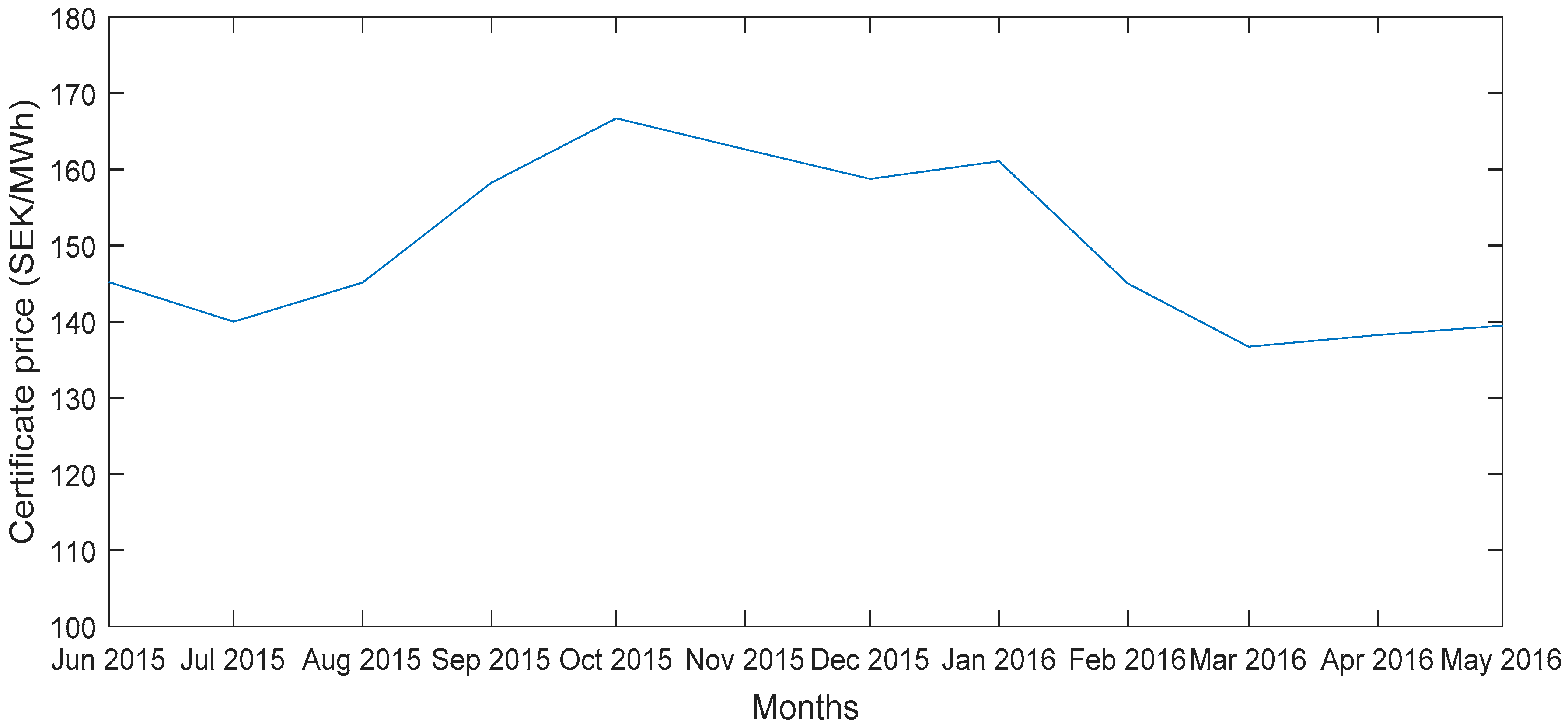
Figure 19.
Monthly average TGC spot prices [39].
Figure 19.
Monthly average TGC spot prices [39].

Figure 20.
Monthly income stream of the wind farm.

Figure 21.
Actual and simulated income of the wind farm.

Figure 22.
Changes in mean output with respect to electricity price and TGC price for January.

Figure 23.
Contribution of electricity price and TGC price to variance of income for January.


Table 1.
Vestas V-27 specifications.
| Rotor | Airfoil | ||
| Diameter | 27 m | Airfoil | NACA 63.214–63.235 |
| Generator-1, rotational speed | 43 RPM | Length | 13 m |
| Generator-2, rotational speed | 33 RPM | Width | 1.3–0.5 m |
| Swept area | 573 m2 | Twist | 13° |
| Diameter | 27 m | Tower | |
| Number of blades | 3 | Height | 30 m |
| Generator–1 | Diameter top | 1.4 m | |
| Rated power | 225 kW | Diameter bottom | 2.4 m |
| Rotational speed | 1008 RPM | Hub height | 31.5 m |
| Rated current | 396 A | Operational Data | |
| Generator–2 | Cut-in speed | 3.5 m/s | |
| Rated power | 50 kW | Rated wind speed | 14 m/s |
| Rotational speed | 760 RPM | Cut-out wind speed | 25 |
| Rated current | 101 A | Rated power | 225 kW |
Table 2.
Wind power class [27].
Table 2.
Wind power class [27].
| Wind Power Class | Description | Power Density at 50 m (W/m2) |
|---|---|---|
| 1 | Poor | 0–200 |
| 2 | Marginal | 200–300 |
| 3 | Fair | 300–400 |
| 4 | Good | 400–500 |
| 5 | Excellent | 500–600 |
| 6 | Outstanding | 600–800 |
| 7 | Superb | 800–2000 |
Table 3.
Monthly wind power class.
| Month | Mean Wind Speed (m/s) | Power Density at 50 m (W/m2) | Wind Power Class |
|---|---|---|---|
| 15 June | 5.36 | 257.5 | 2 |
| 15 July | 4.27 | 126.2 | 1 |
| 15 August | 4.99 | 225 | 2 |
| 15 September | 6.63 | 442 | 4 |
| 15 October | 7.69 | 622.3 | 6 |
| 15 November | 7.42 | 577.4 | 5 |
| 15 December | 9.7 | 1147.6 | 7 |
| 16 January | 9.35 | 1004.6 | 7 |
| 16 February | 6.7 | 429.5 | 4 |
| 16 March | 7.14 | 453.5 | 4 |
| 16 April | 5.24 | 269.6 | 2 |
Table 4.
Properties of (a) target data and (b) reference data.
| (a) | ||
| Property | Original | Processed |
| Start time | 8 May 2015 | 8 May 2015 00:00 |
| End time | 9 May 2016 | 9 May 2016 01:00 |
| Duration | 12 months | 12 months |
| Time step size | 10 min | 60 min |
| No. of Time steps–speed | 51,027 | 8576 |
| No. of Time steps–direction | 50,354 | 8487 |
| (b) | ||
| Property | Original | Processed |
| Start time | 1 January 1980 | 1 January 1980 |
| End time | 1 July 2018 | 1 July 2018 |
| Duration | 12 months | 12 months |
| Time step size | 60 min | 60 min |
| No. of Time steps—speed | 337,464 | 337,464 |
| No. of Time steps—direction | 337,464 | 337,464 |
Table 5.
Comparison of the target and long-term predicted data.
| Property | Target Original | Target Processed | Long-Term Predicted |
|---|---|---|---|
| Start time | 8 May 2015 | 8 May 2015 | 1 January 1980 |
| End time | 9 May 2016 | 9 May 2016 | 1 July 2018 |
| Duration | 12 months | 12 months | 38 years |
| Time-step size | 10 min | 60 min | 60 min |
| No. of time-steps—speed | 51,027 | 8576 | 337,463 |
| No. of time-steps—direction | 50,354 | 8487 | 337,463 |
| Mean speed at hub height | 6.641 m/s | 6.633 m/s | 6.71 m/s |
| MoMM speed at hub height | 6.642 m/s | 6.635 m/s | 6.702 m/s |
| Min. speed at hub height | 0.12 m/s | 0.36 m/s | 0.36 m/s |
| Max. speed at hub height | 27.19 m/s | 25.09 m/s | 30.80 m/s |
| Weibull k at hub height | 1.85 | 1.91 | 2.43 |
Table 6.
Monthly mean power and energy output data.
| Month | Mean Wind Speed (m/s) | Gross Mean Power (kW) | Actual Mean Power (kW) | Gross Mean Energy (kWh) | Actual Mean Energy (kWh) |
|---|---|---|---|---|---|
| 15 June | 5.36 | 42.7 | 38.15 | 30,816 | 27,468 |
| 15 July | 4.27 | 22.3 | 17.92 | 16,591.2 | 1332.5 |
| 15 August | 4.99 | 37.7 | 26.625 | 28,048.8 | 19,809 |
| 15 September | 6.63 | 67.2 | 46.96 | 48,456 | 33,811.2 |
| 15 October | 7.69 | 83.6 | 70.16 | 62,347.2 | 52,199 |
| 15 November | 7.42 | 82.1 | 65.12 | 59,184 | 46,886.4 |
| 15 December | 9.7 | 122.2 | 101.01 | 90,991.2 | 75,151.4 |
| 16 January | 9.35 | 121.0 | 100.24 | 90,098.4 | 74,578.56 |
| 16 February | 6.7 | 67.5 | 59.46 | 47,397.6 | 41,384.2 |
| 16 March | 7.14 | 74.6 | 65.79 | 55,576.8 | 48,947.7 |
| 16 April | 5.24 | 38.3 | 34.38 | 27,648 | 24,753.6 |
| 16 May | 5.35 | 41.6 | 37.21 | 30,950.4 | 27,684.24 |
Table 7.
Parameters for Monte-Carlo simulation.
| Month | Monthly Mean Electricity Prices (SEK/MWh) | Standard Deviation of Electricity Prices (SEK) | Monthly Mean Certificate Prices (SEK/MWh) | Standard Deviation of Certificate Prices (SEK) |
|---|---|---|---|---|
| January | 398 | 151.31 | 225 | 56.357 |
| February | 426 | 209.23 | 226 | 55.8 |
| March | 374 | 142.3 | 222 | 53.34 |
| April | 361 | 99.14 | 219 | 59.236 |
| May | 336 | 80.53 | 216 | 71.89 |
| June | 348 | 103.8 | 210 | 66.49 |
| July | 330 | 125.17 | 212 | 67 |
| August | 365 | 142.24 | 218.919 | 66.12 |
| September | 379 | 162.38 | 222.7 | 68.91 |
| October | 378 | 110.69 | 225 | 68.81 |
| November | 387 | 92.262 | 223 | 60.32 |
| December | 414 | 166.37 | 217 | 53.94100 |
© 2018 by the authors. Licensee MDPI, Basel, Switzerland. This article is an open access article distributed under the terms and conditions of the Creative Commons Attribution (CC BY) license (http://creativecommons.org/licenses/by/4.0/).
Share and Cite
MDPI and ACS Style
Marjan, A.; Shafiee, M. Evaluation of Wind Resources and the Effect of Market Price Components on Wind-Farm Income: A Case Study of Ørland in Norway. Energies 2018, 11, 2955. https://doi.org/10.3390/en11112955
AMA Style
Marjan A, Shafiee M. Evaluation of Wind Resources and the Effect of Market Price Components on Wind-Farm Income: A Case Study of Ørland in Norway. Energies. 2018; 11(11):2955. https://doi.org/10.3390/en11112955
Chicago/Turabian StyleMarjan, Ali, and Mahmood Shafiee. 2018. "Evaluation of Wind Resources and the Effect of Market Price Components on Wind-Farm Income: A Case Study of Ørland in Norway" Energies 11, no. 11: 2955. https://doi.org/10.3390/en11112955
Note that from the first issue of 2016, this journal uses article numbers instead of page numbers. See further details here.