POD Analysis of Entropy Generation in a Laminar Separation Boundary Layer

School of Energy and Power Engineering, Beihang University, Beijing 100191, China
*
Author to whom correspondence should be addressed.
Energies 2018, 11(11), 3003; https://doi.org/10.3390/en11113003
Submission received: 22 September 2018
/
Revised: 20 October 2018
/
Accepted: 26 October 2018
/
Published: 1 November 2018
(This article belongs to the Special Issue Fluid Flow and Heat Transfer)
Abstract
:Separation of laminar boundary layer is a great source of loss in energy and power machinery. This paper investigates the entropy generation of the boundary layer on the flat plate with pressure gradient. The velocity of the flow field is measured by a high resolution and time related particle image velocimetry (PIV) system. A method to estimate the entropy generation of each mode extracted by proper orthogonal decomposition (POD) is introduced. The entropy generation of each POD mode caused by mean viscous, Reynolds normal stress, Reynolds sheer stress, and energy flux is analyzed. The first order mode of the mean viscous term contributes almost 100% of the total entropy generation. The first three order modes of the Reynolds sheer stress term contribute less than 10% of the total entropy generation in the fore part of the separation bubble, while it reaches to more than 95% in the rear part of the separation bubble. It indicates that the more unsteady that the flow is, the higher contribution rate of the Reynolds sheer stress term makes. The energy flux term plays an important role in the turbulent kinetic energy balance in the transition region.
1. Introduction
For the energy and power machinery, such as gas turbine and other turbomachinery, the efficiency must be the most important performance parameters [1]. An effective way to improve efficiency is to reduce the loss, namely to avoid the generation of entropy [2,3,4]. In thermodynamics, any irreversible physical process will inevitably lead to the increase of entropy [5]. In this paper, it mainly focuses on the entropy generation in the boundary layer.
The entropy generation has been the subject of many past studies. Bejan [6], Rotta [7], and McEligot [8] studied the entropy generation in the viscous layer and analyzed the generation rates in diffident Y-plus layer. Moore [9] attempted to develop a numerical model for turbulent flow entropy generation, but Kramer-Bevan [10] verified it is not consistent near the wall due to a small temperature gradient. Adeyinka et al. [11] investigated the error of entropy generation model affected by the mesh grids in the fully-developed laminar flow.
The entropy generation is difficult to be accurately calculated [12]. Since it is difficult to predict the small fluctuating velocity and temperature in the turbulent flow through numerical and experimental [13] few experiments have had sufficient measurements to calculate the entropy generation. Thus, most studies try to estimate the entropy generation with a simplified formulation, which will be introduced in Section 3.2.
To describe and extract coherent structures in boundary layer, researchers attempt to develop new data analysis methods, such as proper orthogonal decomposition (POD), dynamic mode decomposition (DMD), and spectral POD (SPOD). POD is a method that identifies coherent structures by decomposing the flow field into orthogonal modes in space. Moreover, the dominant features in the flow is identified based on the energy rank [14]. Dynamic mode decomposition is a method that is orthogonal in time in the sense that the dynamic mode information from a given flow field is based on the Koopman analysis [15]. In contrast to POD, it is a method that gives the energy of the fluctuations at distinct frequencies meaning the modes are arranged in descending order of energy content. Spectral POD is a method that combines proper orthogonal decomposition with a spectral method to analyze and extract reduced order models of flows from time data series of velocity fields [16].
Since this paper mainly focuses on the entropy generation in the boundary layer. It is more convenient to identify the flow field based on the energy rank and care little about the time series and frequencies. Thus, the POD method is applied to the measurement to estimate the entropy generation. The POD has been widely applied for the experimental and numerical data to identify the coherent structure [17,18], such as the plate boundary layer [19], cylinder engine flow [20], and turbine rotor-stator interaction [21]. Particularly, in the case of laminar separation bubbles, POD can extract the different scale coherent structures [22,23].
While few works have been done to quantify the entropy generation of different coherent structures in the boundary layer. Calculating the entropy generation of those coherent structure helps to explore the mechanisms of entropy generation in the boundary layer. It can also identify the loss resource of the flow flied. In this paper, the entropy generation rate is analyzed by proper orthogonal decomposition (POD) applied to the PIV measurements.
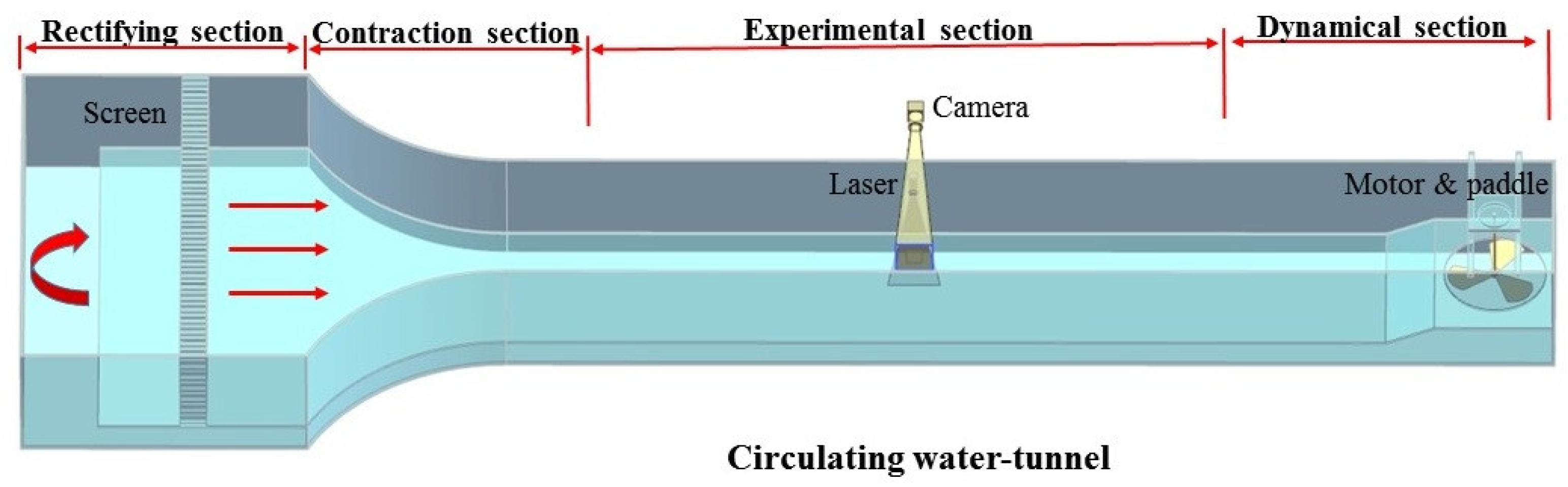
2. Experimental Facility
The measurement is taken in a transparent circulating water tunnel with a 700 mm (width) × 500 mm (depth) experimental section, and the whole length of the water tunnel is 6.8 m, just as Figure 1 shows. The inlet velocity in this experiment is 0.065 m/s. The mean velocity profile in the empty experimental section was uniform except for the thin boundary layers on the walls. The turbulence of the water tunnel is less than 1%, and the Reynolds number is based on the total length of the flat plate and the inlet velocity is about 3 × 10⁴. The flat plate is mounted horizontally in the middle of the water tunnel to ensure zero flow incidence. Total length of the flat plate is 390 mm and the geometrical structure of the leading edge is an ellipse with a ratio of 3:1 to the semi-minor axis length, just as Figure 2 shows.
The instantaneous velocity field of eight streamwise planes (W1–8) is measured by a PIV system. The distance from the first window to the leading edge of the flat plate is 30 mm, and the distance between each windows is 40 mm. The streamwise plane is illuminated by a light sheet provided by a double cavity Nd: YAG laser, which has the maximum illumination energy of 200 mJ/pulse and a maximum repetition rate of 15 Hz. To ensure the PIV system operates in stably, the sampling rate is set as 12 Hz. One thousand pairs of signal-exposure images are continuously captured by a CCD camera with a resolution of 2072 pixels × 2072 pixels, and the reality view window is about 38.5 mm × 38.5 mm. The PIV measurement uncertainty can refer to the paper [24], in which the same PIV system is used. A more detailed investigation of the uncertainty in the turbulent boundary layer can be found in [25].
3. Dara Processing Method
3.1. POD Method
Since any turbulent flow can be viewed as a superposition of a small number of coherent structures, the equations describing these structures can be considered in a low-dimensional description of turbulence. The POD is an effective method to extract these coherent structures. The time related flow field snapshots can be decomposed into a linear basis set consisting of N basis function (POD mode) and the corresponding coefficients (POD coefficients or time coefficients). The POD mode provides the spatial information on coherent structures, and the POD coefficients retain the temporal information. In addition to those two parameters, the eigenvalues represents the total kinetic energy that each POD mode captured. The original flow field can be reconstructed by POD mode and POD coefficients.
The instantaneous velocity of kth POD mode is:
The mean velocity of kth POD mode is:
The velocity fluctuation of kth POD mode is:
Thus, the Reynolds stresses of kth POD mode can be computed as:
3.2. Estimation of Entropy Generation
Basic thermodynamics tells us that entropy generates when the process is irreversible such as viscous friction [1]. The viscous dissipation is a main frictional irreversibility in boundary layers, which includes mean viscous dissipation and turbulent dissipation. So the entropy generation can be expressed as:
where the mean viscous dissipation is [2]:
The turbulent dissipation is:
Rotta [7] gives a simple estimation function of entropy generation:
Since, the energy flux term plays an important role in the turbulent energy balance in the transition, so it should also take the energy flux term into account in entropy generation. Thus, the entropy generation can be calculated as following form [7,26,27]:
where the first term on the right side of Equation (10) is the viscous term, the second term is the Reynolds shear stress term, the third term is the Reynolds normal stress term; the fourth term is the energy flux term, the fifth term is the turbulent diffusion term, and the last term is the pressure diffusion term. As the last two terms are small, comparing to the magnitudes of other terms, so it can be neglected [26]. All above equations are widely used to estimate the entropy generation especial in experimental work. Since it does not involve the pressure and temperature, only the instant velocity should be measured. It is easy to measure the instant velocity through PIV, hotline probe, and LDV.
3.3. Effect of Decomposition Region Size on POD
In order to explore the effect of decomposition region size on POD results, different decomposition region size has been investigated. The results of four different height cases are shown in Figure 3. It shows that, when the height of the decomposition region is less than 30 mm, the spatial structure of different windows is consecutive, but the symbols of the velocity in W5 and W6 are reverse at different cases. When the height reaches to 35 mm, the POD can even not extract the structure of boundary layer in window 5. This is mainly because the POD extracts a coherent structure according to the total kinetic energy of the flow field. The first-order mode captures more than 99% of the energy at W5 and W6, as shown in Figure 4; the higher-order modes naturally capture a very low energy. Therefore, the higher order modes are easily to be effect by the disturbance in main flow. In W7 and W8, the energy distribution is more uniform because of a more unsteady boundary layer, so it shows more stabilization with different decomposition region sizes. For the same reasons, the size of streamwise decomposition region has the same effect on the POD results, which is not shown in this paper. Thus, in order to extract more flow field structure and avoid the effect of main flow disturbance on the POD mode, the decomposition region size in following work is all 30 mm × 38.5 mm (only shows 20 mm × 38.5 mm).
4. Results and Discussion
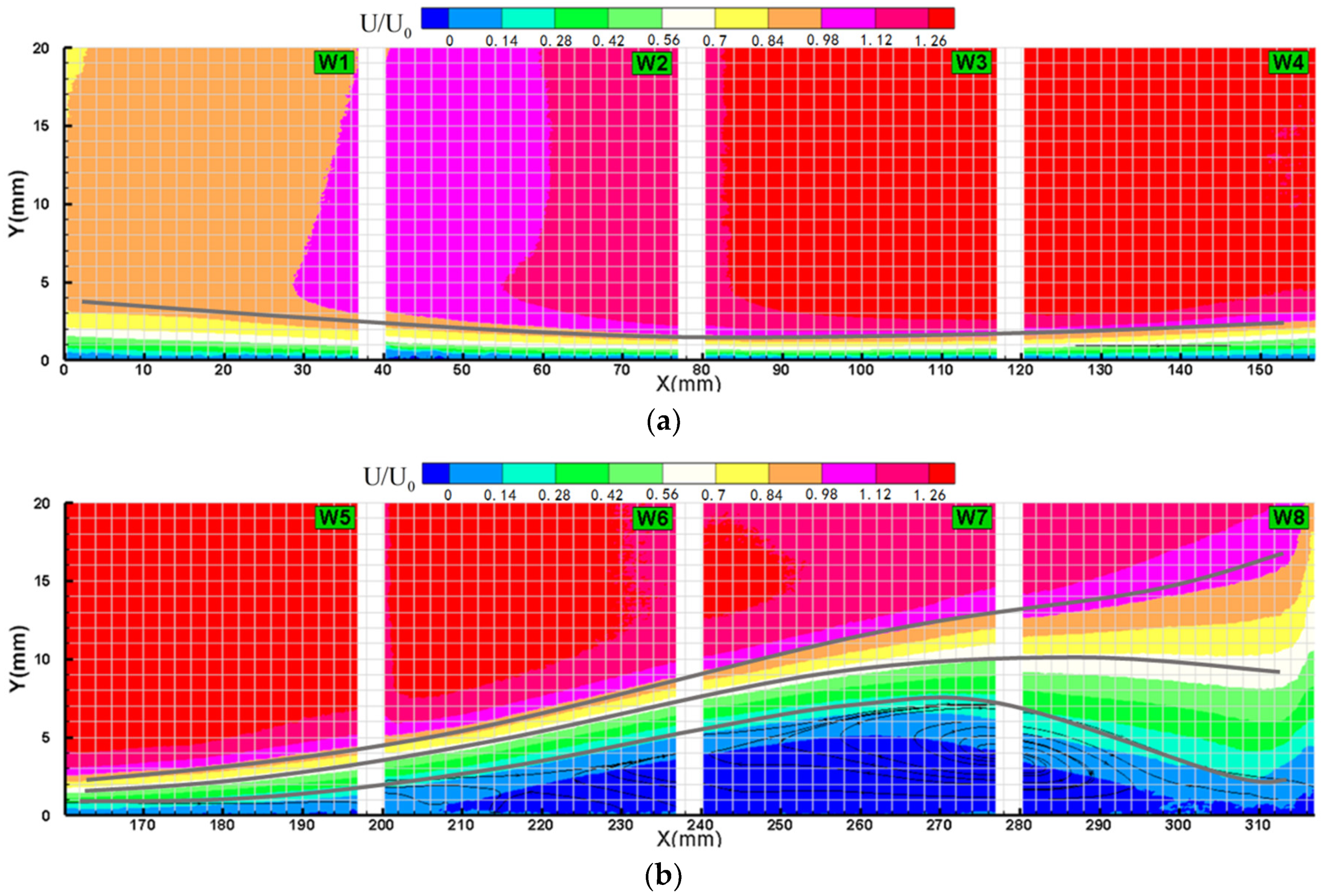
4.1. Time-Mean Flow Field
Figure 5 shows the time-mean flow field on the flat plate. The thickness of boundary layer decreases gradually with the velocity increase under the favorable pressure gradient, and then increases rapidly under the adverse gradient. The boundary layer separates at about X = 200 mm, and it reattaches again at the end of the outlet, where the adverse gradient is disappearance. It forms a time-mean separation bubble in the separated boundary layer, while for the temporary flow field, it consists of a series of vortex. In [28], some criteria can be used to assess if flow history (upstream evolution of the streamwise pressure gradient) have an impact on the development of the boundary layer. The following analyses concentrates on the aft portion of the flat plate boundary layer downstream of the transition.
Figure 6 shows the normalized velocity pattern of the boundary layer along the streamwise. It is easy to judge the state of the boundary layer through the velocity pattern. The boundary layer at = 41–46 is a typical attached boundary layer. There is no inflexion point in the velocity pattern, which indicates that the flow at those positions has not yet separated. From the position of = 47.5, the velocity pattern has obvious inflection point. It indicates that the boundary layer has separated. The height of the inflection point also represents the boundary of the separation bubble shown as the dotted line in Figure 6.
Figure 7 shows the variation of boundary layer thickness, displacement boundary layer thickness, momentum boundary layer thickness and the shape factor along the streamwise. What should be noted that strong pressure gradient may lead to an inconsistent boundary layer edge by the common techniques to define the boundary layer edge [29]. The shape factor maintains about 2 to 3 in W1–3, where the boundary layer keeps laminar. The boundary layer separates at the position of X = 200 mm, the value of the shape factor just consistent with the typical value of the separation laminar boundary. Between the laminar region and the separation region, there is a transition region. Downstream of the transition region, the shape factor increase rapidly due to the increase of the displacement boundary layer thickness. The shape factor start to decrease from the location of X = 260 mm, the position corresponds the maximum thickness of the separation bubble.
4.2. POD Analysis of Flow Field
Figure 8 shows the different POD modes of the streamwise velocity. The flow structure of the first order mode is consistent with the time-mean flow field. Since the flow field is almost steady in W5 and W6, the flow structure of different modes is a little similar to each other, while in W7 and W8, the flow structure of different modes is much different from each other because of strong unsteady. The second order mode is still the large-scale coherent structures that affected by the mean flow. The third–fourth-order modes represent the small coherent structures that induced by the large-scale vortex, and the coherent structure paired increases with the increase of the order number [30].
Figure 9 shows the power spectrum density of the POD coefficient, which represents the turbulent kinetic energy of the POD mode. There is a basic frequency (0.024 Hz) in the power spectrum of the POD coefficient, which corresponds with the frequency of the main flow turbulence. The energy mainly concentrates in a low frequency band for those four windows. The amplitude of the energy spectrum increases gradually from W5 to W8 with the increasing unsteady of the flow. The energy at high frequency decreases faster and faster from W5 to W8. The slope of the forth order mode at W8 tends to be −3/5, which indicates that the flow field of the forth order mode tends to be fully developed turbulent flow.
According to the Equations (2)–(5), the Reynolds stress of different POD modes are calculated and shown in Figure 10. The distribution of the first order mode Reynolds stress is basically consistent with the original flow field (not given in this paper), which also verifies the correctness of the above equations. The extracted Reynolds normal stress of mode 2 and mode 3 mainly distributes above the separation bubble, while the Reynolds shear stress distributes in the whole boundary layer.
4.3. Entropy Generation Analysis
4.3.1. Entropy Generation of Original Flow Field
According to the Equation (10), the different entropy generation terms are calculated and shown in Figure 11. It shows that the magnitude of the mean viscous dissipation term is much smaller than other terms. The entropy of the mean viscous dissipation only generates in laminar boundary layer and the edge of the separation bubble. Since the velocity in the separation bubble is very small, the entropy generation tends to be very small in the separation bubble. Nevertheless, it does not mean that the separation bubble will not cause any loss. The separation bubble will induce a rapidly increase of the boundary layer thickness and the Reynolds stress dissipation loss in the separated boundary layer is much higher than that of the attached boundary layer, just as Figure 11 shows. The energy flux term distributes in the whole main flow and there is not a clear boundary between the positive area with the negative area.
Figure 12 shows the variation of the integrated entropy generation in the boundary along the streamwise. In the laminar region (W1–3), the entropy generation of the laminar boundary layer keeps at a very low level. In the transition region (W4), the amplitude of the energy flux term increases significantly. It indicates that the energy flux term plays an important role in the turbulent kinetic energy balance. The integrated energy flux shows discontinuity between windows and data sparsity, which results from the discrete distribution of energy flux term in the counter map just as the Figure 11 shows. Figure 13 shows the total integrated entropy generation in the boundary layer. It shows that the total entropy generation increases significantly when the boundary layer separated. The Reynolds shear stress term tends to be positive growth and the energy flux term is negative growth, which is consistent with the trend described in [27].
4.3.2. Entropy Generation of POD Mode
As described above, the POD is an effective method to extract the coherent structures. The entropy generation of the coherent structures extracted by POD can be calculated through Equations (2)–(5) and (10). It significant to quantize the entropy generation of the coherent structures. Once you can identify the source of the coherent structures, then the source of the loss production can be confirmed [31].
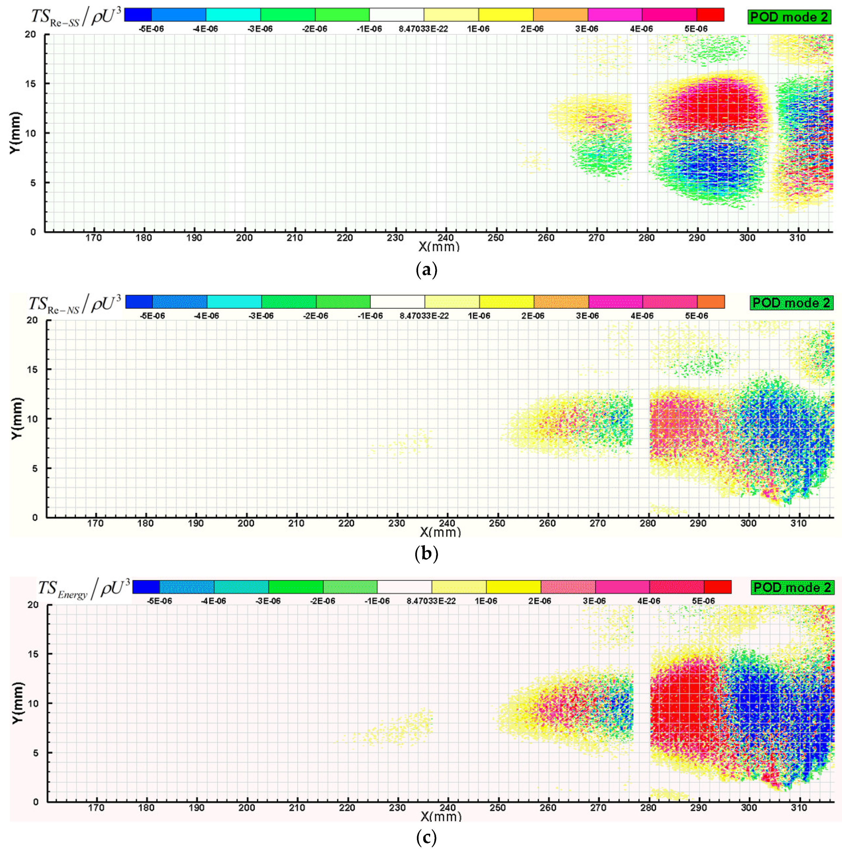
Figure 14, Figure 15 and Figure 16 show the entropy generation of different POD modes. The first-order mode of the mean viscous dissipation term is almost equal to that of the original flow field and the value of higher order mode tends to be zero. It also demonstrates that the first order mode represents the mean flow. The entropy generation distribution of the second and third-order mode of the Reynolds stress term and the energy flux term is similar to the distribution of the related POD mode.
Figure 17 shows the cumulative contribution to the total integral entropy generation of each POD mode in the boundary layer. The contribution rate of the first order mode of the mean viscous term reaches 100% in all of those windows. In W5, the contribution rate of the first two modes of the Reynolds stress (normal and sheer) is about 10%, the magnitude of the higher modes is almost at the same level. Thus, the contribution of each mode seems to be the same and the cumulative contribution line increases with a constant slope. The Reynolds sheer stress term in W6 has the same situation with that in W5, while the first third-order mode of the Reynolds normal stress in W6 contributes about 80% of the total entropy generation. The contribution rate of the energy flux term reaches to 90% until the cumulative order number of the POD mode is about 400 in both W5 and W6.
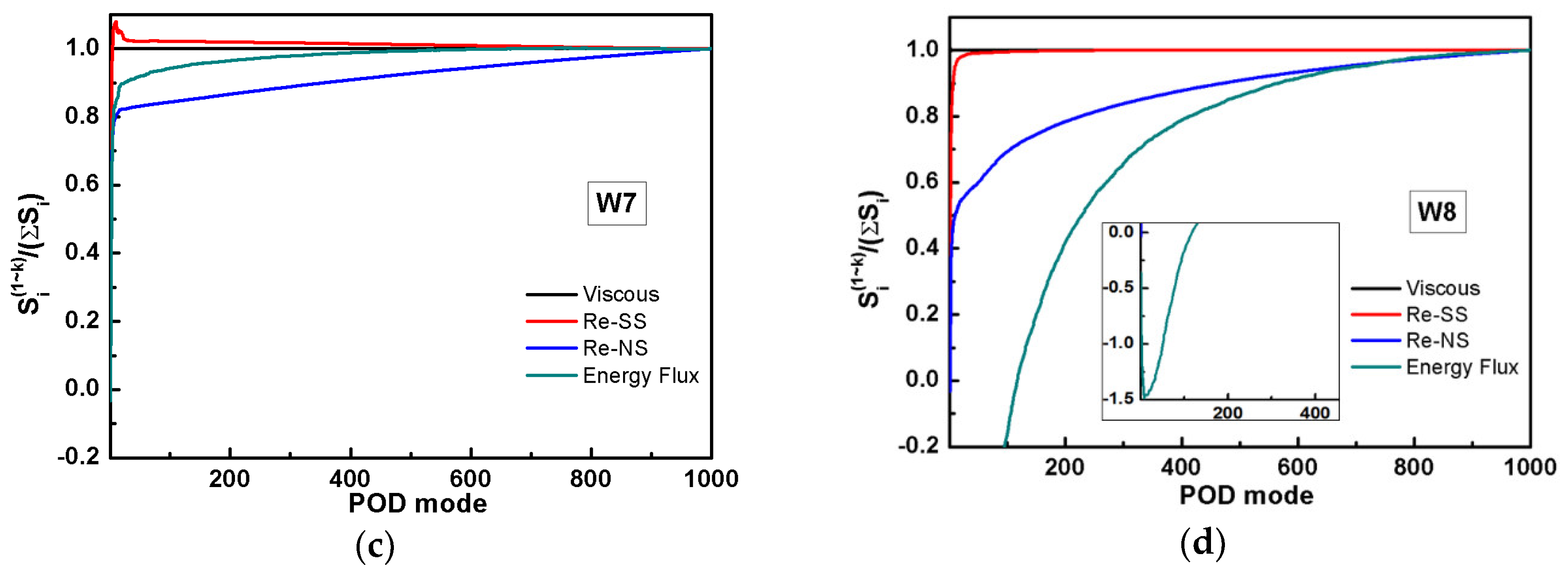
In W7, the first third-order modes of Reynolds stress (normal and sheer) term contributes more than 80% of the total entropy generation, the higher order contributes less than 20%. In W8, the contribution of the first 30th-order modes of the Reynolds stress (normal and sheer) is about 60%. It indicates that the contribution of the Reynolds stress term of the low-order mode in the rear part of the separation bubble (W7 and W8) is much higher than that in the fore part of the separation bubble (W5). The low order mode of the energy flux term in W8 contributes the negative value, which results from the negative energy captured by the first-order mode just as shown in Figure 16.
5. Conclusions
In this paper, the boundary layer of the flat plate with a pressure gradient in the water tunnel has been studied using high-resolution particle image velocimetry (PIV). The entropy generation rate is analyzed by proper orthogonal decomposition (POD) applied to the measurements. Several conclusions can be made.
The separation bubble will dramatically increase the thickness of the boundary layer and result in a sharp increase of the loss. The loss due to the Reynolds normal stress mainly distributes above the separation bubble, and the loss due to the Reynolds shear stress distributes in the whole boundary layer. The decomposition region size has a significantly effects on the POD result of the laminar boundary layer. It should reduce the proportion of the main flow area as much as possible when carrying out the POD analysis. In the transition region, the energy flux terms plays an important role in transiting the energy from the mean flow to the turbulent flow and contributes a large ratio to the entropy generation. Estimation of the entropy generation of the POD mode helps to explore the mechanism of entropy generation and identify the source of the loss production. Additionally, it is easy to promote this method to some other complex flows, such as wake-induced separation on the suction side of blade, or the leakage flow on the blade tip from either numerical or experimental data, which is only based on the instantaneous velocity field.
Author Contributions
Conceptualization: C.J.; data curation: C.J.; investigation: C.J.; methodology: C.J.; software: C.J.; supervision: H.M.; validation: C.J.; writing—original draft: C.J.; writing—review and editing: H.M.
Funding
This study was supported by the National Natural Science Foundation of China (Grant No. 51776011).
Conflicts of Interest
The authors declare no conflict of interest.
Nomenclature
| Shape factor | |
| Reynolds number | |
| Entropy generation | |
| Temperature | |
| Instantaneous streamwise velocity | |
| Streamwise velocity fluctuation () | |
| Averaged streamwise velocity | |
| Streamwise velocity of main flow | |
| Instantaneous spanwise velocity | |
| Spanmwise velocity fluctuation () | |
| Averaged spanwise velocity | |
| POD coefficients | |
| Eigenvalue of POD | |
| Basis function of POD | |
| Density | |
| Kinetic viscosity | |
| Kinematic viscosity | |
| Boundary layer thickness | |
| Displacement boundary layer thickness | |
| Momentum boundary layer thickness |
References
- Denton, J.D. The 1993 IGTI Scholar Lecture: Loss Mechanisms in Turbomachines. J. Turbomach. 1993, 115, 621–656. [Google Scholar] [CrossRef]
- Bejan, A.; Kestin, J. Entropy Generation through Heat and Fluid Flow. J. Appl. Mech. 1983, 50, 475. [Google Scholar] [CrossRef]
- Naterer, G.F.; Camberos, J.A. Entropy Based Design and Analysis of Fluids Engineering Systems; CRC Press: Boca Raton, FL, USA, 2008. [Google Scholar]
- Bejan, A. Entropy Generation Minimization; Advanced Engineering Thermodynamics; John Wiley & Sons, Inc.: Hoboken, NJ, USA, 1995. [Google Scholar]
- Enrico, S. Calculating entropy with CFD. Mech. Eng. 1997, 119, 86–88. [Google Scholar]
- Suder, K.L.; Obrien, J.E.; Reshotko, E. Experimental Study of Bypass Transition in a Boundary Layer; National Aeronautics & Space Administration Report; NASA: Washington, DC, USA, 1988.
- Rotta, J.C. Turbulent boundary layers in incompressible flow. Prog. Aerosp. Sci. 1962, 2, 1–95. [Google Scholar] [CrossRef]
- Mceligot, D.M.; Walsh, E.J.; Laurien, E.; Spalart, P.R. Entropy Generation in the Viscous Parts of Turbulent Boundary Layers. J. Fluids Eng. 2008, 130, 61205. [Google Scholar] [CrossRef]
- Moore, J.; Moore, J.G. Entropy Production Rates from Viscous Flow Calculations: Part I—A Turbulent Boundary Layer Flow. In Proceedings of the ASME 1983 International Gas Turbine Conference and Exhibit, Phoenix, AZ, USA, 27–31 March 1983. [Google Scholar]
- Kramer-Bevan, J.S. A Tool for Analyzing Fluid Flow Losses. Master’s Thesis, University of Waterloo, Waterloo, ON, Canada, 1992. [Google Scholar]
- Adeyinka, O.B.; Naterer, G.F. Apparent Eentropy Production Difference with Heat and Fluid Flow Irrevesibilities. Numer. Heat Transf. Part B Fundam. 2002, 42, 411–436. [Google Scholar] [CrossRef]
- Adeyinka, O.B.; Naterer, G.F. Modeling of Entropy Production in Turbulent Flows. J. Fluids Eng. 2005, 126, 893–899. [Google Scholar] [CrossRef]
- Hanjalić, K.; Launder, B. Modelling Turbulence in Engineering and the Environment; Cambridge University Press: Cambridge, UK, 2000. [Google Scholar]
- Lumley, J.L. Stochastic Tools in Turbulence; Dover Publications: Mineola, NY, USA, 2007. [Google Scholar]
- Schmid, P.; Sesterhenn, J. Dynamic mode decomposition of experimental data. In Proceedings of the 8th International Symposium on Particle Image Velocimetry, Melbourne, Australia, 25–28 August 2009. [Google Scholar]
- Cammilleri, A.; Gueniat, F.; Carlier, J.; Pastur, L.; Mémin, E.; Lusseyran, F.; Artana, G. POD-spectral decomposition for fluid flow analysis and model reduction. Theor. Comput. Fluid Dyn. 2013, 27, 787–815. [Google Scholar] [CrossRef] [Green Version]
- Zhu, J.; Huang, G.; Fu, X.; Fu, Y.; Yu, H. Use of POD Method to Elucidate the Physics of Unsteady Micro-Pulsed-Jet Flow for Boundary Layer Flow Separation Control. In Proceedings of the ASME Turbo Expo 2013: Turbine Technical Conference and Exposition, San Antonio, TX, USA, 3–7 June 2013. [Google Scholar]
- Hammad, K.J. Coherent Structures in Turbulent Boundary Layer Flows over a Shallow Cavity. In Proceedings of the ASME 2017 International Mechanical Engineering Congress and Exposition, Tampa, FL, USA, 3–9 November 2017. [Google Scholar]
- Anbry, N. The dynamics of coherent structures in the wall region of a turbulent boundary layer. J. Fluid Mech. 1988, 192, 115–173. [Google Scholar]
- Chen, H.; Reuss, D.L.; Sick, V. On the use and interpretation of proper orthogonal decomposition of in-cylinder engine flows. Meas. Sci. Technol. 2012, 23, 085302. [Google Scholar] [CrossRef]
- Cizmas, A.; Paul, G.; Palacios, A. Proper Orthogonal Decomposition of Turbine Rotor-Stator Interaction. J. Propuls. Power 2003, 19, 268–281. [Google Scholar] [CrossRef]
- Lengani, D.; Simoni, D. Recognition of coherent structures in the boundary layer of a low-pressure-turbine blade for different free-stream turbulence intensity levels. Int. J. Heat Fluid Flow 2015, 54, 1–13. [Google Scholar] [CrossRef]
- Lengani, D.; Simoni, D.; Ubaldi, M.; Zunino, P.; Bertini, F. Experimental Investigation on the Time–Space Evolution of a Laminar Separation Bubble by Proper Orthogonal Decomposition and Dynamic Mode Decomposition. J. Turbomach. 2016, 139, 31006. [Google Scholar] [CrossRef]
- Tian, Y.; Ma, H.; Wang, L. An Experimental Investigation of the Effects of Grooved Tip Geometry on the Flow Field in a Turbine Cascade Passage Using Stereoscopic PIV. In Proceedings of the ASME Turbo Expo 2017: Turbomachinery Technical Conference and Exposition, Charlotte, NC, USA, 26–30 June 2017. [Google Scholar]
- Vinuesa, R.; Schlatter, P.; Nagib, H.M. Role of data uncertainties in identifying the logarithmic region of turbulent boundary layers. Exp. Fluids 2014, 55, 1751. [Google Scholar] [CrossRef]
- Walsh, E.J.; Mc Eligot, D.M.; Brandt, L.; Schlatter, P. Entropy Generation in a Boundary Layer Transitioning under the Influence of Freestream Turbulence. J. Fluids Eng. 2011, 133, 61203. [Google Scholar] [CrossRef]
- Skifton, R.S.; Budwig, R.S.; Crepeau, J.C.; Xing, T. Entropy Generation for Bypass Transitional Boundary Layers. J. Fluids Eng. 2017, 139, 041203. [Google Scholar] [CrossRef]
- Vinuesa, R.; Orlu, R.; Vila, C.S.; Ianiro, A.; Discetti, S.; Schlatter, P. Revisiting History Effects in Adverse-Pressure-Gradient Turbulent Boundary Layers. Flow Turbul. Combust. 2017, 99, 565–587. [Google Scholar] [CrossRef] [PubMed] [Green Version]
- Vinuesa, R.; Bobke, A.; Örlü, R.; Schlatter, P. On determining characteristic length scales in pressure-gradient turbulent boundary layers. Phys. Fluids 2016, 28, 55101. [Google Scholar] [CrossRef]
- Vila, C.S.; Orlu, R.; Vinuesa, R.; Schlatter, P.; Ianiro, A.; Discetti, S. Adverse-Pressure-Gradient Effects on Turbulent Boundary Layers: Statistics and Flow-Field Organization. Flow Turbul. Combust. 2017, 99, 589–612. [Google Scholar] [CrossRef] [PubMed] [Green Version]
- Lengani, D.; Simoni, D.; Ubaldi, M.; Zunino, P.; Bertini, F.; Michelassi, V. Accurate Estimation of Profile Losses and Analysis of Loss Generation Mechanisms in a Turbine Cascade. J. Turbomach. 2017, 139, 121001–121007. [Google Scholar] [CrossRef]
Figure 1.
Water tunnel and experimental layout.

Figure 2.
Placement of the PIV camera windows.
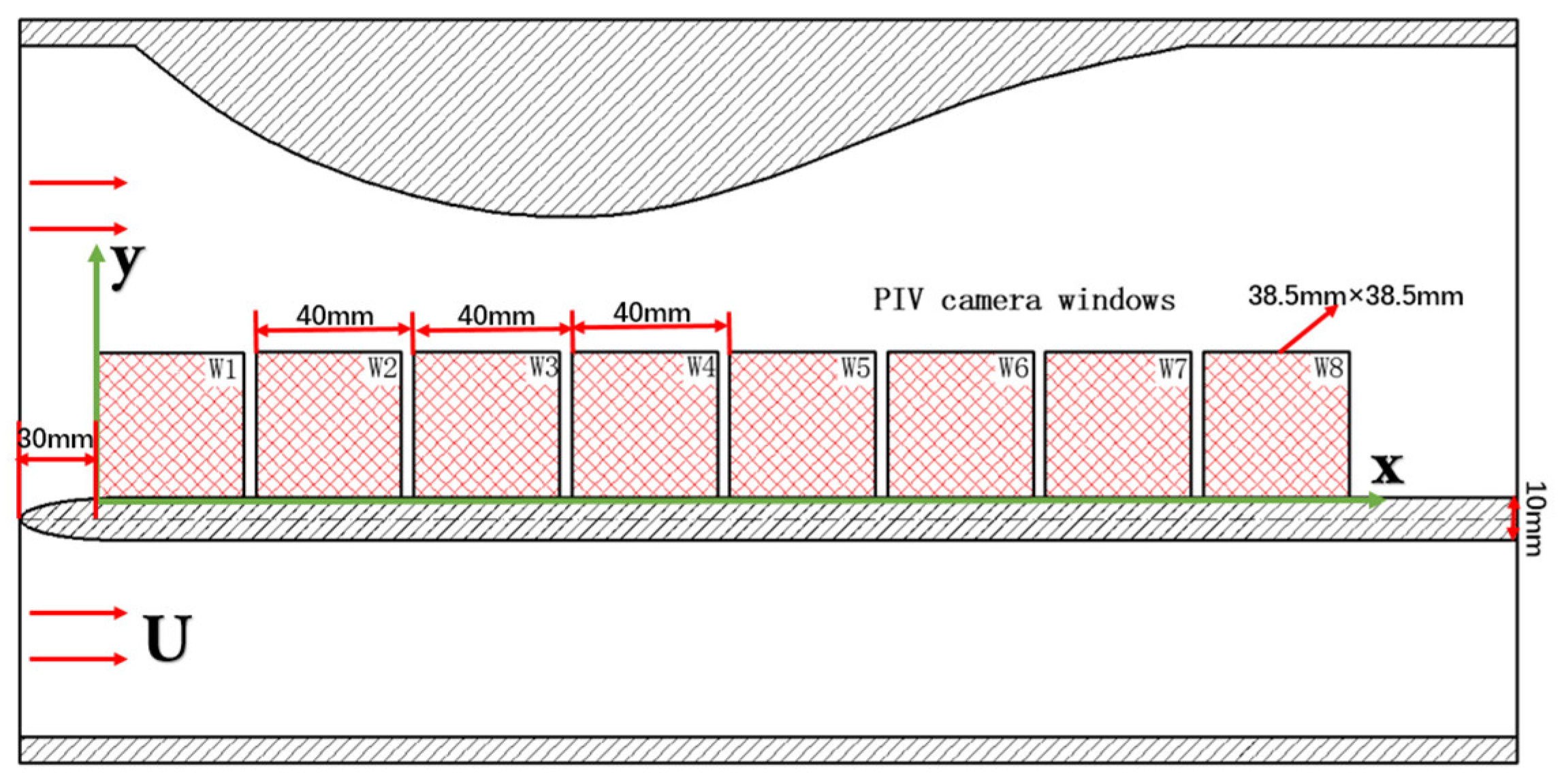
Figure 3.
The third-order mode of the streamwsie velocity with different spanwise decomposition region size: (a) H = 20 mm; (b) H = 25 mm; (c) H = 30 mm; and (d) H = 35 mm.
Figure 3.
The third-order mode of the streamwsie velocity with different spanwise decomposition region size: (a) H = 20 mm; (b) H = 25 mm; (c) H = 30 mm; and (d) H = 35 mm.
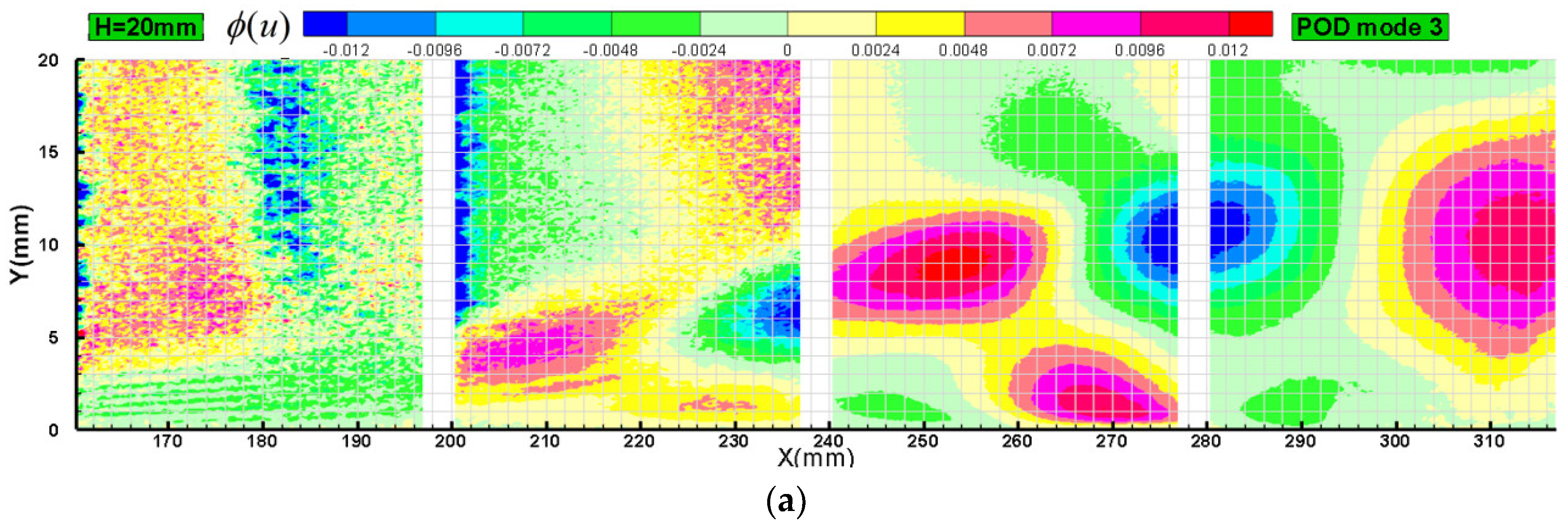
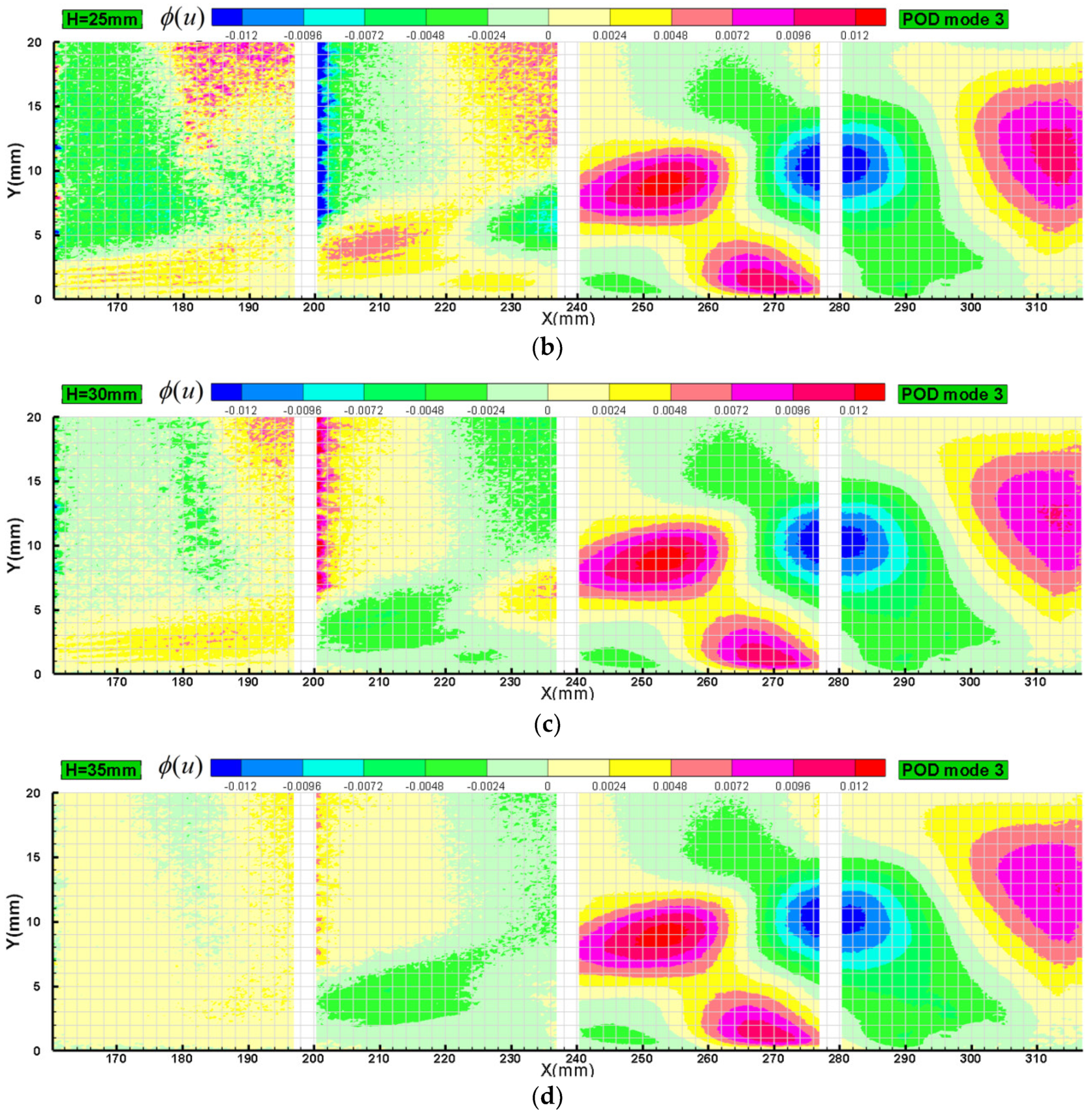
Figure 4.
Contribution to total energy of the first order POD mode.
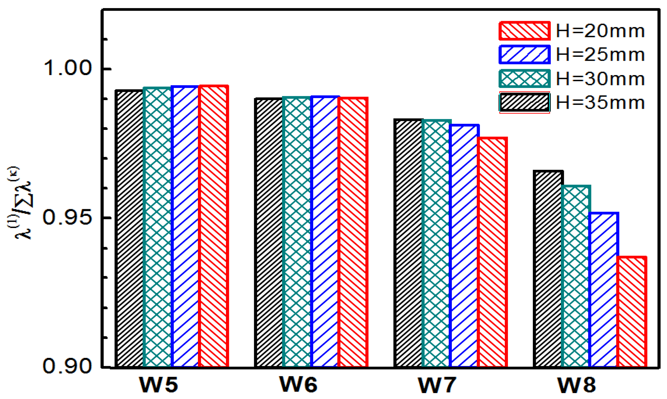
Figure 5.
Time mean streamwise velocity: (a) the fore part of the flow field; and (b) the rear part of the flow field.
Figure 5.
Time mean streamwise velocity: (a) the fore part of the flow field; and (b) the rear part of the flow field.

Figure 6.
Normalized velocity of the boundary layer.
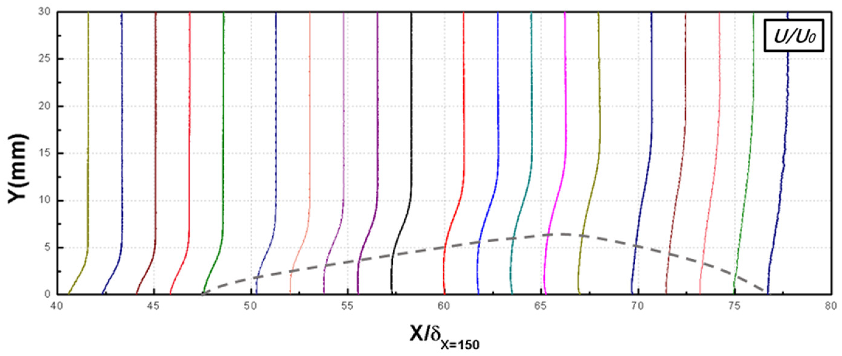
Figure 7.
Streamwise variation of the boundary layer parameters.
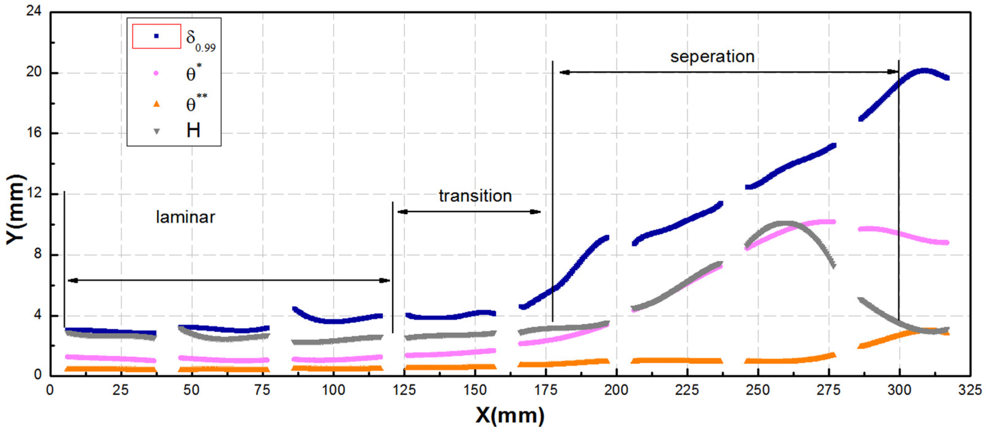
Figure 8.
POD modes of streamwise velocity: (a) the first order mode; (b) the second order mode; (c) the third order mode; and (d) the forth order mode.
Figure 8.
POD modes of streamwise velocity: (a) the first order mode; (b) the second order mode; (c) the third order mode; and (d) the forth order mode.

Figure 9.
Power spectrum density of the POD coefficient: (a) W5; (b) W6; (c) W7; and (d) W8.
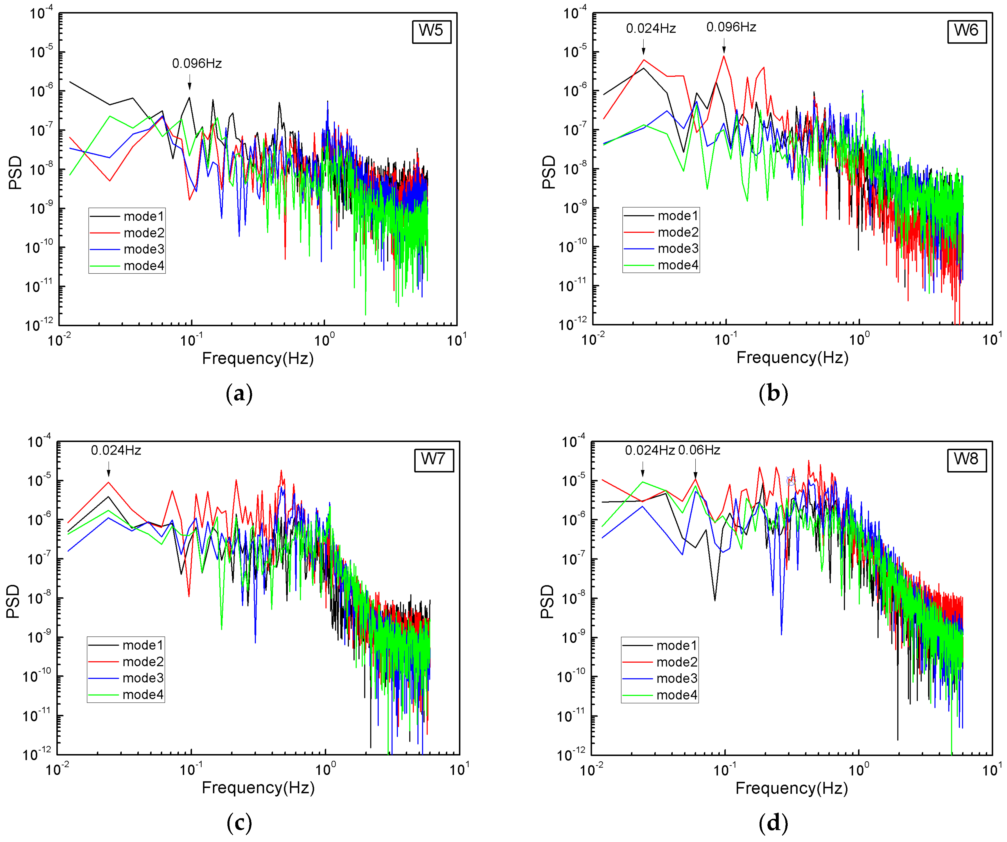
Figure 10.
(a) The second-order mode of the Reynolds normal stress; (b) the third-order mode of the Reynolds normal stress; (c) the second-order mode of the Reynolds sheer stress; and (d) the third-order mode of the Reynolds sheer stress.
Figure 10.
(a) The second-order mode of the Reynolds normal stress; (b) the third-order mode of the Reynolds normal stress; (c) the second-order mode of the Reynolds sheer stress; and (d) the third-order mode of the Reynolds sheer stress.
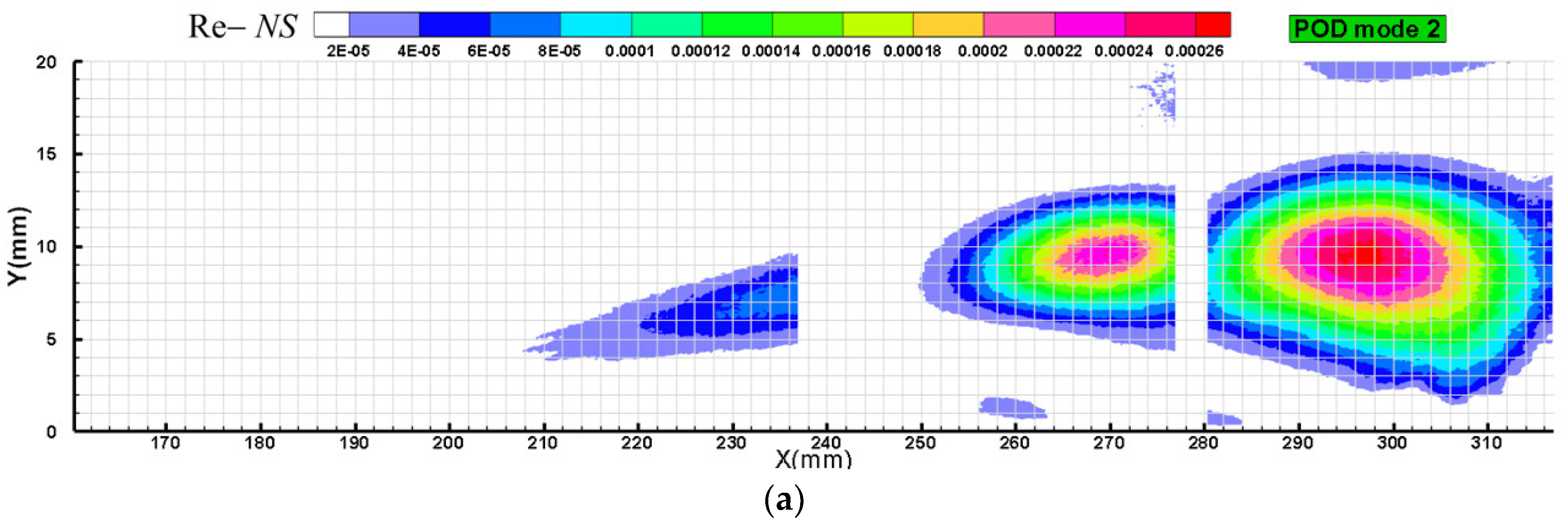
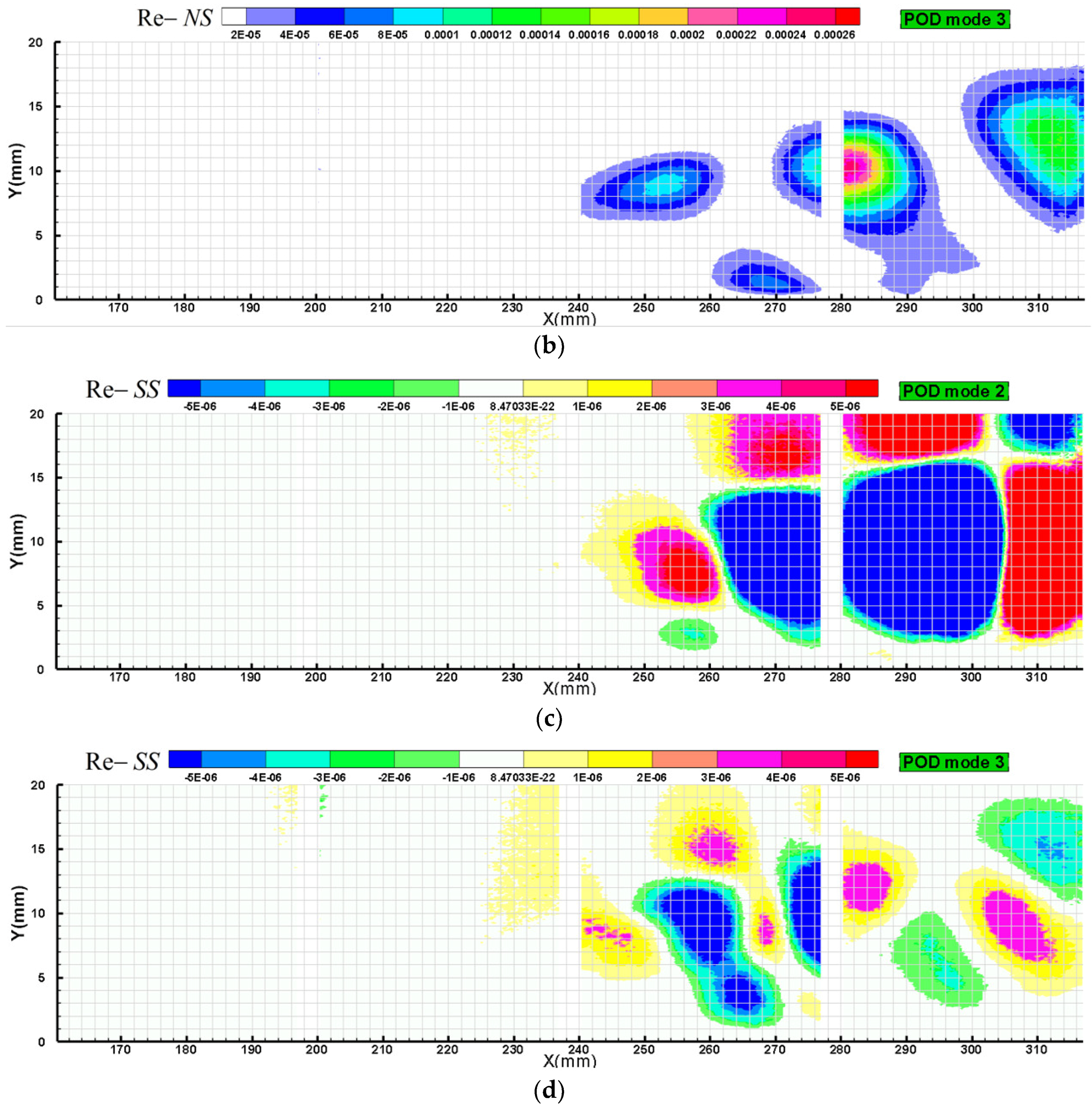
Figure 11.
Distribution of different terms of entropy generation: (a) the mean viscous dissipation term; (b) the Reynolds sheer stress term; (c) the Reynolds normal stress term; and (d) the energy flux term.
Figure 11.
Distribution of different terms of entropy generation: (a) the mean viscous dissipation term; (b) the Reynolds sheer stress term; (c) the Reynolds normal stress term; and (d) the energy flux term.
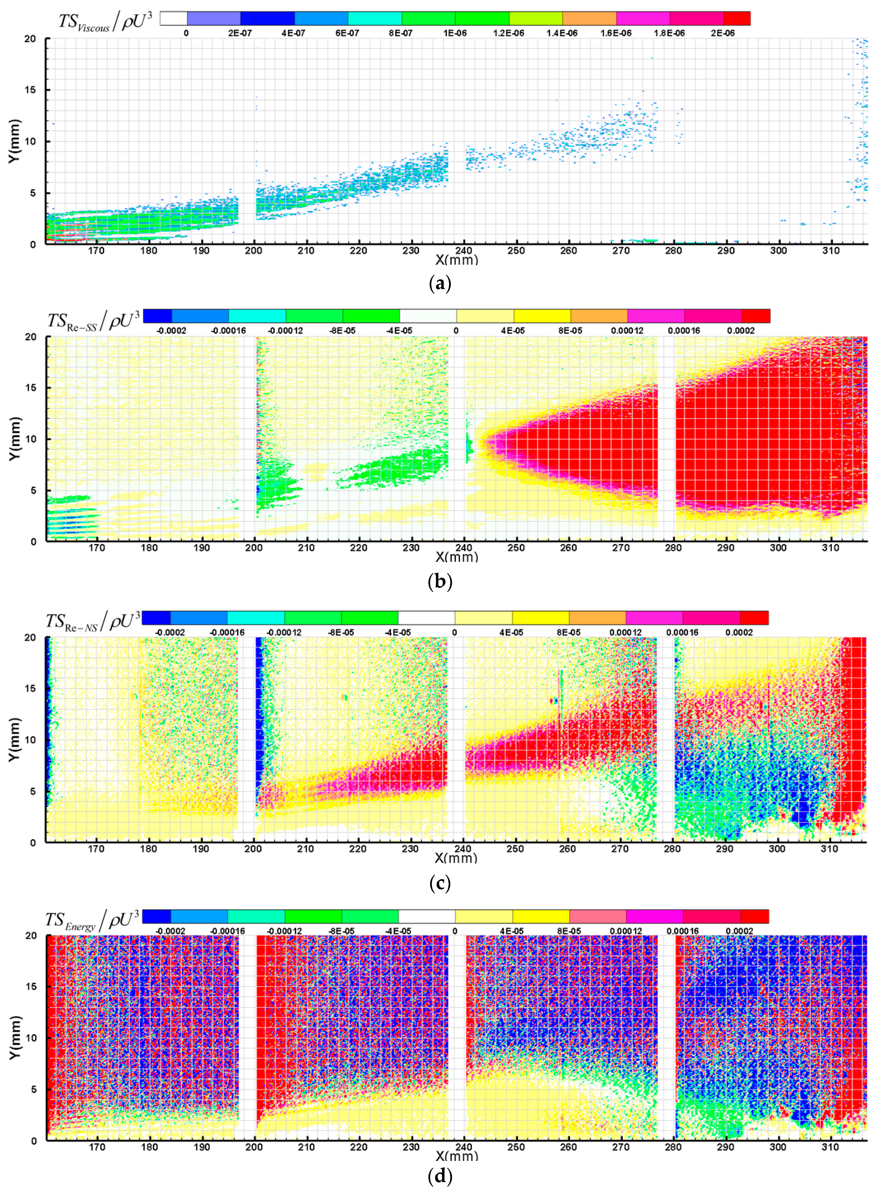
Figure 12.
Streamwise variation of integral entropy generation.
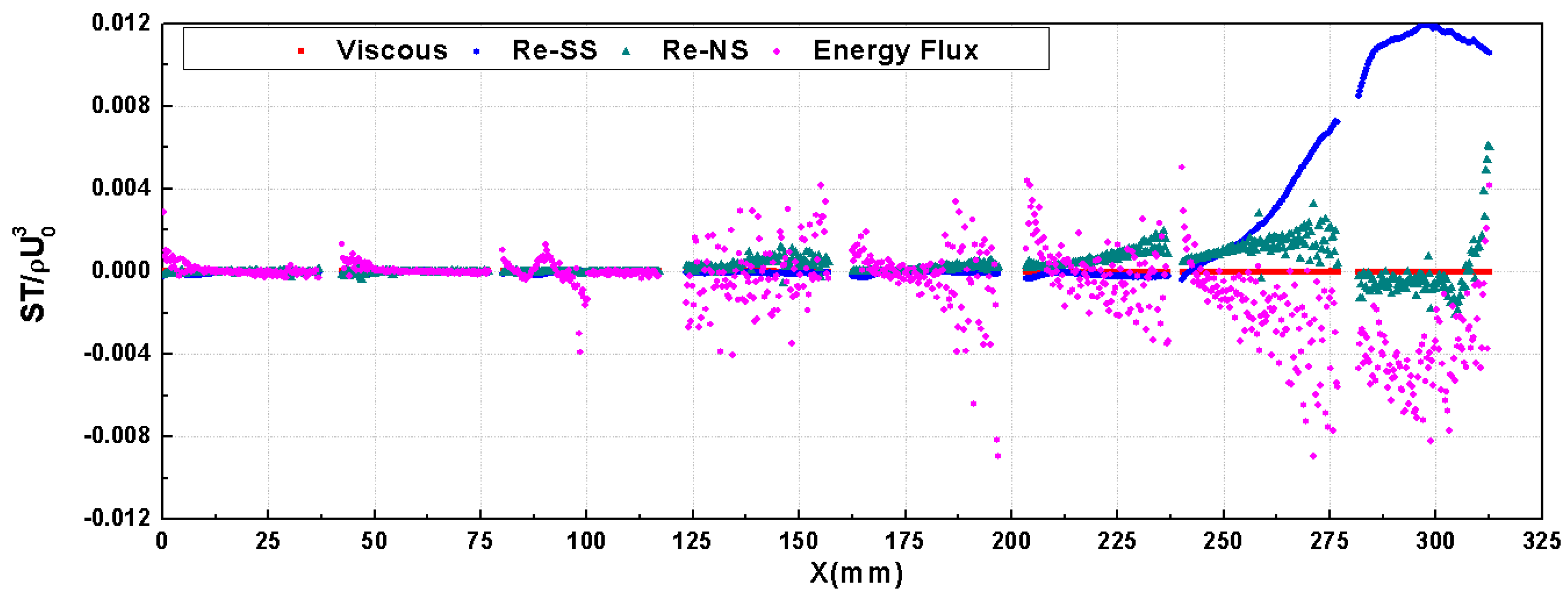
Figure 13.
Total integral entropy generation of different terms.
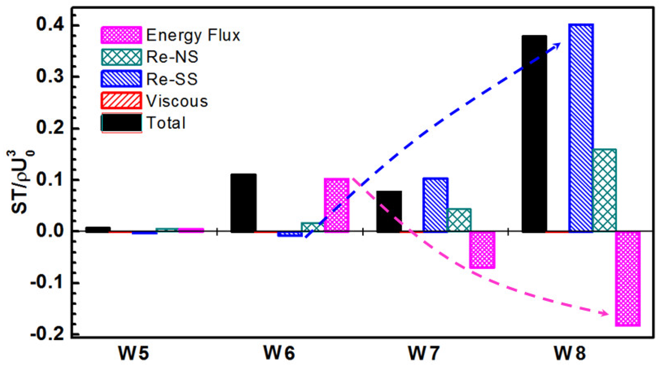
Figure 14.
Entropy generation of first order mode: (a) the mean viscous dissipation term; (b) the Reynolds sheer stress term; (c) the Reynolds normal stress term; and (d) the energy flux term.
Figure 14.
Entropy generation of first order mode: (a) the mean viscous dissipation term; (b) the Reynolds sheer stress term; (c) the Reynolds normal stress term; and (d) the energy flux term.
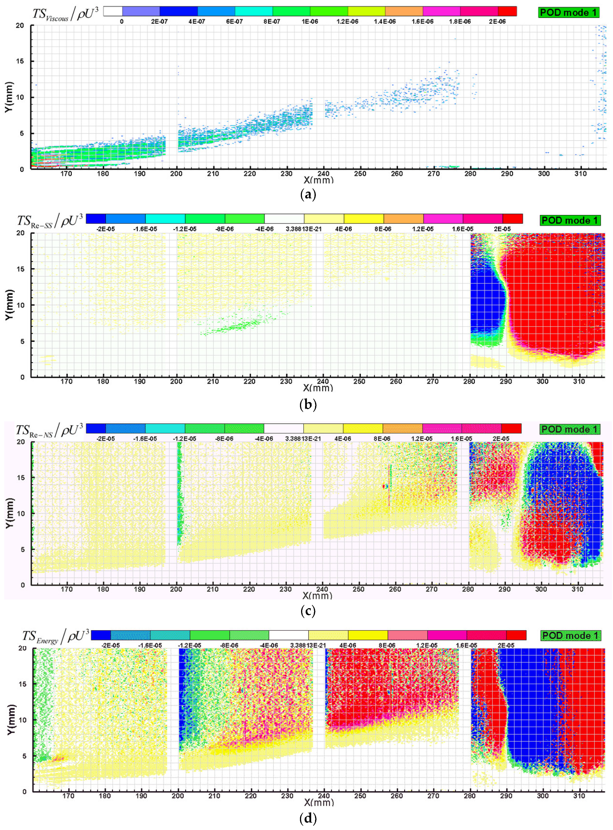
Figure 15.
Entropy generation of second order mode: (a) the Reynolds sheer stress term; (b) the Reynolds normal stress term; and (c) the energy flux term.
Figure 15.
Entropy generation of second order mode: (a) the Reynolds sheer stress term; (b) the Reynolds normal stress term; and (c) the energy flux term.

Figure 16.
Entropy generation of third order mode: (a) the Reynolds sheer stress term; (b) the Reynolds normal stress term; and (c) the energy flux term.
Figure 16.
Entropy generation of third order mode: (a) the Reynolds sheer stress term; (b) the Reynolds normal stress term; and (c) the energy flux term.


Figure 17.
Cumulative contribution to the total integral entropy generation of each POD mode: (a) W5; (b) W6; (c) W7; and (d) W8.
Figure 17.
Cumulative contribution to the total integral entropy generation of each POD mode: (a) W5; (b) W6; (c) W7; and (d) W8.

© 2018 by the authors. Licensee MDPI, Basel, Switzerland. This article is an open access article distributed under the terms and conditions of the Creative Commons Attribution (CC BY) license (http://creativecommons.org/licenses/by/4.0/).
Share and Cite
MDPI and ACS Style
Jin, C.; Ma, H. POD Analysis of Entropy Generation in a Laminar Separation Boundary Layer. Energies 2018, 11, 3003. https://doi.org/10.3390/en11113003
AMA Style
Jin C, Ma H. POD Analysis of Entropy Generation in a Laminar Separation Boundary Layer. Energies. 2018; 11(11):3003. https://doi.org/10.3390/en11113003
Chicago/Turabian StyleJin, Chao, and Hongwei Ma. 2018. "POD Analysis of Entropy Generation in a Laminar Separation Boundary Layer" Energies 11, no. 11: 3003. https://doi.org/10.3390/en11113003
Note that from the first issue of 2016, this journal uses article numbers instead of page numbers. See further details here.