Investigation on the Handling Ability of Centrifugal Pumps under Air–Water Two-Phase Inflow: Model and Experimental Validation

Abstract

The paper presents experimental and numerical investigations performed on a single stage, single-suction, horizontal-orientated centrifugal pump in air–water two-phase non-condensable flow conditions. Experimental measurements are performed in a centrifugal pump using pressure sensor devices in order to measure the wall static pressures at the inlet and outlet pump sections for different flow rates and rotational speeds combined with several air void fraction (a) values. Two different approaches are used in order to predict the pump performance degradations and perform comparisons with experiments for two-phase flow conditions: a one-dimensional two-phase bubbly flow model, and a full “Three-Dimensional Unsteady Reynolds Average Navier–Stokes” (3D-URANS) simulation using a modified k-epsilon turbulence model combined with the Euler–Euler inhomogeneous two-phase flow description. The overall and local flow features are presented and analyzed. Limitations concerning both approaches are pointed out according to some flow physical assumptions and measurement accuracies. Some additional suggestions are proposed in order to improve two-phase flow pump suction capabilities.

1. Introduction

Pumps play an important role in many energy engineering applications. Their main advantages are their high operational efficiency and reliability. In case of inlet two-phase flow conditions such as irrigation, refrigeration, petroleum, nuclear power industries, sewage treatment, etc., pump performance always fails under air–water two-phase inflow compared to single-phase operations. Especially, the need for the safe operation and design of a nuclear power reactor is of paramount importance to assure the safety evaluation of hypothetical loss-of-coolant accidents (LOCA) in light water reactors. Therefore, the investigation of pump behavior during blowdown is very important.

The degree of head degradation depends on the geometrical, physical, and thermal conditions. Compared with an axial flow pump that is able to suck high inlet gas volume fraction values, centrifugal pumps are less powerful when handling two-phase flow conditions (Gülich [1]). When the inlet gas void fraction increases, the pump head can be totally lost, and this often results in huge system instabilities and pump failure. Such a situation should be controlled using adequate prediction methods. Some improvements on pump ability to suck two-phase flow can also be achieved by a better understanding of local flow features. Several models have been developed in order to predict the two-phase flow performance of both the axial and centrifugal types of pumps. A first correlation was proposed in 1978 by Mikielewicz et al. [2], based on the concept of apparent loss coefficient. Among several theoretical approaches, the one-dimensional two-phase flow models proposed by Murakami et al. [3] and Minemura et al. [4] are still considered sufficiently accurate for engineering purposes for the prediction of pump surge or shut-off conditions.

A non-exhaustive list of important published works is proposed in the paper of Si et al. [5]. Related proposed models can be considered to be valid for low values of inlet void fraction (maximum 6–7% in volume). They cannot accurately predict the surge operating conditions that correspond to a rapid decrease in the pump performance, just because they only give mean flow characteristics along one mean streamline with no local information inside the impeller whole passage. Just before such severe conditions, several investigations have also detected the presence of stationary bubbles at impeller entrance channels for high gas fractions, being responsible for the starting point of the strong performance degradation of the pump (Sekoguchi et al. [6], Estevam et al. [7] and Barrios [8]). Numerical simulations, using the so-called “Three-Dimensional Unsteady Reynolds Average Navier–Stokes” (3D-URANS) approach, have also been applied to describe local phenomena more precisely in such flow conditions. They generally show significant deviations between predicted and experimental overall results when inlet void fraction values are higher than 6%. Recently, Müller et al. [9] have performed numerical calculations using a monodispersed phase distribution model, the results of which are compared with the experimental results obtained by Suryawijaya and Kosyna [10]. The comparison of impeller blade static pressure distributions showed that some improvements should be done for a high inlet gas flow rate in order to get a better fit between the numerical and experimental results. This means that there is still a need for experimental results on low specific speed pump geometries in order to obtain more data for numerical assessments.

The present paper presents a compilation of new experimental and numerical analysis performed by the same research team, starting from three years ago by Si et al. [5,11]. In the first part, the measured overall performances of the pump (head and global efficiency versus flow coefficients) are presented for three different rotational speeds and different inlet void fraction values up to pump breakdown. The results are then compared with the one-dimensional two-phase flow model developed by Minemura et al. [4]. In the second part, a comparison is proposed between the experimental results and 3D-URANS simulations using inhomogeneous flow model assumption. Based on the local flow feature analysis obtained from 3D-URANS simulations, radial impeller design modification is proposed to improve pump ability with respect to multiphase flows.

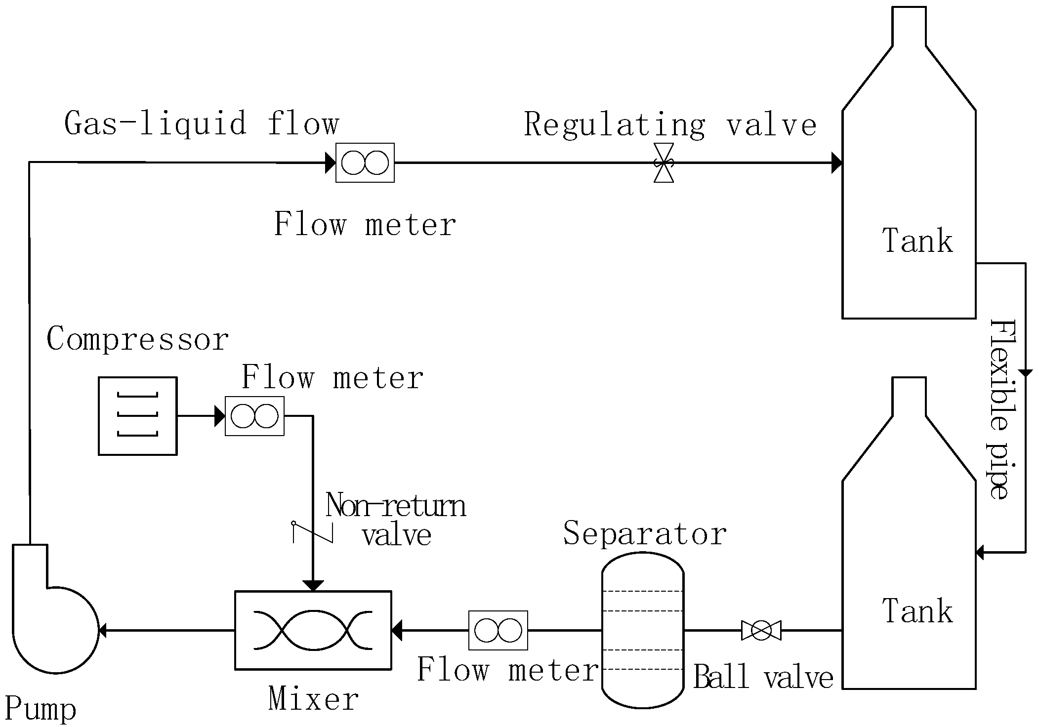
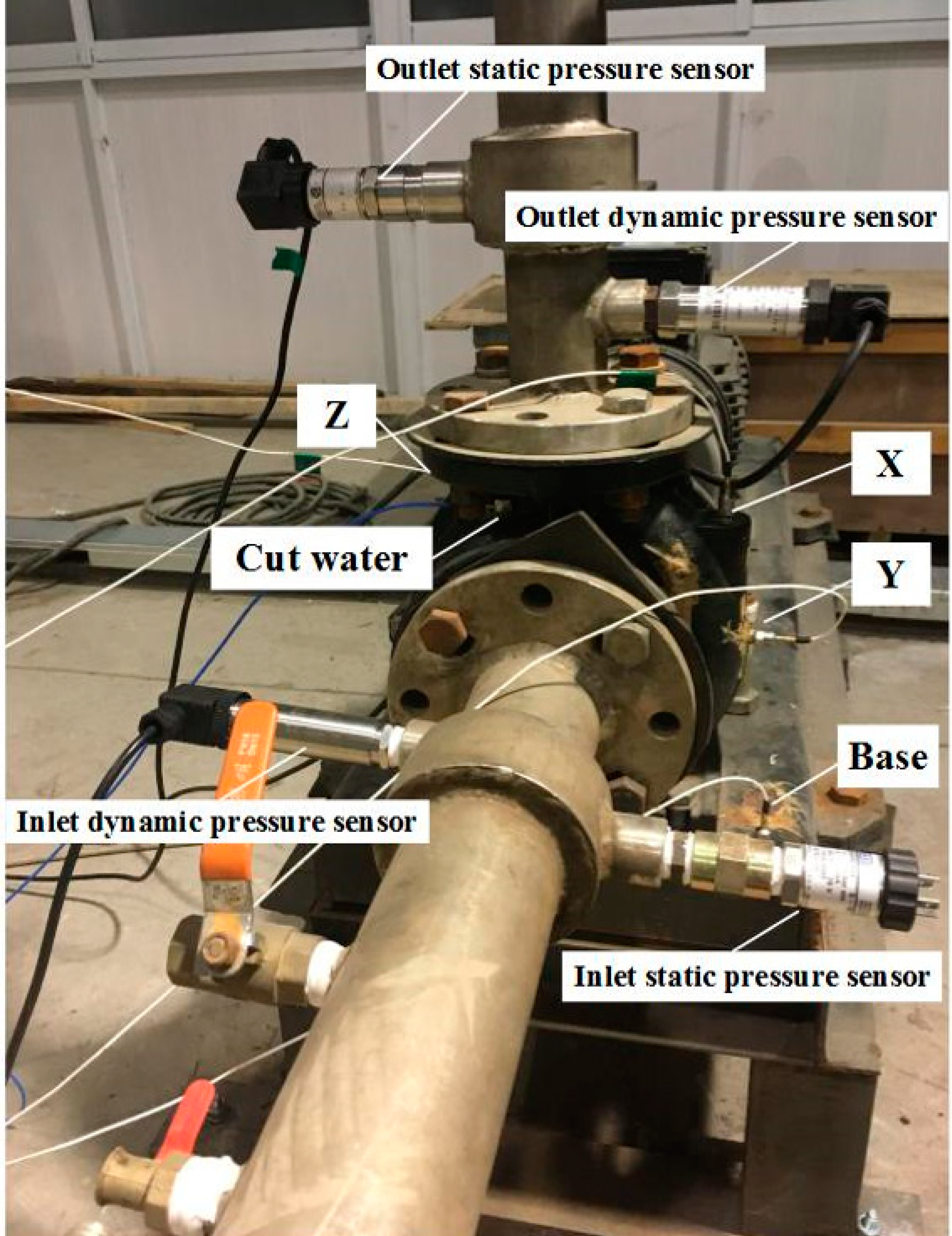
2. Pump Geometry and Experimental Test Rig

A single stage, low specific speed (Ωs = 0.65) centrifugal commercial pump is chosen for two-phase flow investigations. The impeller casing is combined with a vaneless spiral volute. The design parameters of the pump, given by the manufacturer, are as follows: design volume flow rate: Q_d = 50.6 m³/h, design head: H_d = 20.2 m, design speed N_d = 2910 r/min, pump horizontal inlet tube diameter: D = 65 mm. The impeller inlet and outlet diameters are equal to 79 mm and 140 mm, respectively, and the impeller outlet width is equal to 15.5 mm. The six blades’ inlet geometry corresponds to a three-dimensional twisted shape. The volute’s law evolution obeys the Archimedes’ spiral shape. The test rig is shown in Figure 1. As shown in this open loop, the air injection system is able to provide 0.2 mm diameter bubbles using a specific compressor device (more details can be found in Si et al. [5,11]). The air flow rate is measured by a microelectromechanical flow sensors system that could supply the volume air flow rate value on standard conditions (25 °C, 101.326 kPa). A gas–liquid flow mixture is sucked by the pump, goes through the regulating valve, and finally goes into the downstream tank. This open tank allows air bubbles to be separated from the water up to a second tank (upstream tank). The water flow rate was measured by an electromagnetic flowmeter set between the upstream tank and the air supply device. Measurements were performed using the followed procedure: a constant inlet void fraction was set by changing the throttle vane position and the corresponding water flow rate was consequently obtained. Measurement uncertainties are evaluated as a 1.2% error on the pump head and a 2.4% error regarding pump global efficiency. Figure 2 shows a general view of the sensor locations close to the pumping environment. Pump head and global efficiency values were obtained following ISO 9906:2012. It has to be noticed that only the air volume flow rate was measured at this step, as the bubble diameter distribution, including bubble number per unit volume at pump inlet, was not available.

3. Numerical Model and Setups

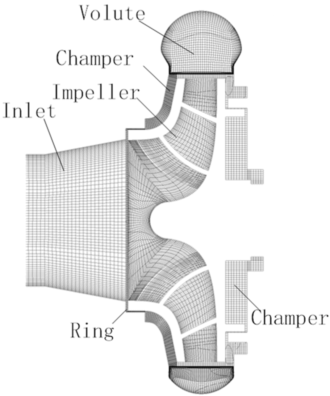
3.1. Model and Mesh

Software Pro/E 5.0 was used for three-dimensional modeling and assembly. The computational domain included five separated domains: inlet pipe, ring, impeller, volute, and disc chambers, as illustrated in Figure 3. The hexahedron structured mesh was used to easily control the density of each node and properly adjust all of the nodes. In order to improve the accuracy of the simulation, the boundary layer grid was added on the volute shell wall after the local encryption of the volute tongue. The resulting pump model that consisted of 2,775,915 elements was chosen for rotating and stationary domains in total after grid independence analysis (see the paper of Si et al. [11]), the result of which is shown in Figure 4.

3.2. The Eulerian–Eulerian Inhomogeneous Two-Phase Flow Model

There are two kinds of multiphase flow models: homogeneous and inhomogeneous ones. The former assumes that the two-phase velocities are the same, not considering any velocity slip between the two phases. The latter considers not only the velocity slip, but also the interphase mass and momentum transfer terms. In the inhomogeneous model, each phase has its own fluid field and passes through the phase transfer unit. That is to say, each phase has its own velocity and temperature field, if any. This paper adopts the inhomogeneous model regardless of the temperature field, for which the liquid phase is continuous and the gas phase is discrete. The particle model assumes that the gas–liquid two-phase flow pattern corresponds to a bubbly flow, meeting the principle of the mass and momentum conservation:

$$\frac{\partial }{\partial t}({\alpha }_k{\rho }_k)+\nabla \cdot ({\alpha }_k{\rho }_k{\mathit{w}}_k)=0$$

(1)

$$\frac{\partial }{\partial t}({\alpha }_k{\rho }_k{\mathit{w}}_k)+\nabla \cdot ({\alpha }_k{\rho }_k{\mathit{w}}_k\otimes {\mathit{w}}_k)=-{\alpha }_k\nabla p_k+\nabla \cdot ({\alpha }_k{\mu }_k(\nabla {\mathit{w}}_k+{(\nabla {\mathit{w}}_k)}^{\mathrm{T}}))+{\mathit{M}}_k+{\mathit{f}}_k$$

(2)

where k—phase (l-liquid, g-gas); ρ_k—density of the k phase, kg/m³; p_k—pressure of k phase, Pa; α_k—void fraction of k phase; μ_k—dynamic viscosity of k phase, Pa·s; w_k—relative velocity of the k phase fluid, m/s; M_k—due to interphase drag force; and f_k—added mass force related to the contribution of the impeller rotation.

This also satisfied:

$${\alpha }_{\mathrm{g}}=1-{\alpha }_{\mathrm{l}}=\frac{Q_{\mathrm{g}}}{Q_{\mathrm{g}}+Q_{\mathrm{l}}}$$

(3)

where α_g—gas void fraction; α_l—liquid void fraction; Q_g—volume flow rate of the gas, m³/h; and Q_l—volume flow rate of the liquid, m³/h.

For this two-phase flow approach, the liquid phase is considered the continuous phase using a modified turbulence model that is based on the renormalization group (RNG) k-ε model [12]. Meanwhile, the gas phase is considered as the discrete phase using the zero-equation theoretical model, which means the action between the two phases only considers the so-called interfacial drag coefficient through the following relations [13]:

$$M_l=-M_g=\frac{3}{4}{c}_D\frac{{\rho }_l}{d_B}{\alpha }_g\left(w_g-w_l\right)\left|w_g-w_l\right|$$

(4)

with:

$$c_D=\{\begin{array}{ll}\frac{24}{R_e}(1+0.15R{e}^{0.687})& (R_e\le 1000)\\ 0.44& (R_e>1000)\end{array}$$

(5)

$$\mathrm{And}Re={\rho }_l\frac{\left|w_g-w_l\right|}{{\mu }_l}{d}_B$$

(6)

where d_B—diameter of the bubble, c_D—resistance coefficient.

3.3. The Modified Turbulence Model

As known, the turbulence model plays a significant role in the prediction of pumping two-phase flow. Since two-phase flow in centrifugal pumps is also an unsteady multiphase compressible flow concerning a liquid phase and a bubble phase, a corrected method was applied to solve that physical phenomenon. This method was proved effective on the prediction of cavitation flow in centrifugal pumps by Wang et al. [14]. The liquid density is defined as:

$${\rho }_{\mathrm{l}}={\rho }_{ref}\sqrt[n]{\frac{p+C}{p_{ref}+C}}$$

(7)

where P_ref stands for the reference pressure at different void fraction, and ρ_ref is set as 998.2 kg/m³. As for constant values of C and n, they are set to 300 MPa and seven for water, respectively, according to Dular and Coutier-Delgosha [15].

Moreover, the standard k–e model is deemed to overestimate the eddy viscosity in the mixture region. It cannot effectively resolve the detachment of the flow separation from the solid surface, and excessively attenuates the two-phase flow instability. Therefore, a modified RNG k–e model, as proposed by Coutier-Delgosha et al. [16], was employed in this work. It can successfully reduce the eddy viscosity by defining the turbulent viscosity, and based on RNG k-$\epsilon$ turbulence model, Johansen’s filter-based model is used to correct the turbulent viscosity ${\mu }_t$:

$${\mu }_t=f\left({\rho }_m\right)C_{\mu }\frac{k^2}{\epsilon }$$

(8)

where f(ρ_m) is the expression of the density correction which can be determined as:

$$f\left({\rho }_m\right)=\{\begin{array}{ll}998.2\mathrm{kg}/{\mathrm{m}}^3& (n=1)\\ {\rho }_g+\frac{{\left({\rho }_m-{\rho }_g\right)}^n}{{\left({\rho }_l-{\rho }_g\right)}^{n-1}}& (n>1)\end{array}$$

(9)

where f(ρ_m) changed with the density of the mixed flow following the rules, as shown in Figure 5. Coutier-Delgosha et al. [16] validated that n should be equal to 10 after comparing the experimental and numerical results.

Finally, the modified RNG k-ε turbulence model becomes as follows:

$$\frac{\partial \left({\rho }_{m}k\right)}{\partial t}+\frac{\partial \left({\rho }_{m}k\overline{u_j}\right)}{\partial x_j}=\frac{\partial }{\partial x_j}\left[\left({\mu }_m+\frac{{\mu }_t^{\prime }}{{\sigma }_k}\right)\frac{\partial k}{\partial x_j}\right]+P_t-{\rho }_m\epsilon$$

(10)

$$\frac{\partial \left({\rho }_m\epsilon \right)}{\partial t}+\frac{\partial \left({\rho }_m\epsilon u_i\right)}{\partial x_i}=\frac{\partial }{\partial x_j}\left[\left({\mu }_m+\frac{{\mu }_t^{\prime }}{{\sigma }_{\epsilon }}\right)\frac{\partial \epsilon }{\partial x_j}\right]+C_{\epsilon 1}\frac{\epsilon }{k}-C_{\epsilon 2}{\rho }_m\frac{{\epsilon }^2}{k}-R$$

(11)

Solutions of the simulations were processed in Ansys CFX 14.1 by adding the modified coefficients programs using CFX Expression Language (CEL).

3.4. Boundary Conditions

Considering the requirements of the test, the inlet boundary conditions are set according to the pressure measured in the experiment. A certain amount of gas is imported into the inlet, and the outlet boundary conditions are set as the mass flow rate. The liquid boundary adopts the non-slip solid wall condition, and the gas boundary adopts the free-slip solid wall condition. The smooth wall condition is used for the near-wall function. The initial inlet bubble diameter is set as 0.2 mm, according to the experimental setup device. The time step was set as 1.718 × 10⁻⁴ s, corresponding to a 3° impeller rotation for each step. A total time set was 0.206 s for simulated results storage in order to further process a data reduction of the unsteady flow field, corresponding to 10 impeller revolutions for which stable results were obtained.

4. Overall Pump Performances

In previous experimental work [5], as well as for pure water, pump head and global efficiency curves were found to be independent of rotational speed inside the range of 1800–2910 r/min. This result agrees with the similarity laws that have been applied for incompressible flow for impeller Reynolds number values (based on impeller diameter and angular speed) that are higher than the critical one that is usually adopted for turbomachinery applications. The rotational speed of 2910 r/min corresponds to the rated one. This result was achieved by considering that the maximum experimental error is 6% for the head at partial flow rates, and 2% around the maximum efficiency point (experimental error combines both measurement device accuracy and local unsteadiness due to two-phase flow stability problems).

Figure 6 shows the experimental pump performance head coefficient ψ_tp (defined in Equation (12)) versus flow coefficient φ for different inlet void fraction values for the rated rotational speed. The corresponding theoretical head curve coefficient obtained with different rotational speeds is shown in Figure 7.

$${\psi }_{tp}=\frac{gH}{u_2^2}(\frac{{\rho }_l}{{\rho }_g\times \alpha +{\rho }_l\times (1-\alpha )})$$

(12)

$${\psi }_{tp,th}={\psi }_{tp}/\eta$$

(13)

As already pointed out by several previous researchers, pump performance starts to be significantly lower when the void fraction reaches 3% or more. The value of the head performance degradation also depends on the flow coefficient. For a given loop characteristic curve, both the head and volume flow rate decrease when a increases. A decrease in 20% in the head coefficient compared with single phase shut-off conditions is achieved for all of the water flow rates that are below nominal conditions when a reach 7%. A maximum a value, which is close to 10%, can be achieved without pump surge for a water flow coefficient around 0.065–0.077. These values correspond to flow rate values between 34–40 m³/h, which are close to the pump-measured best efficiency (reached at φ = 0.084) for single-flow operations. Pump performance sharply drops when a is more than 8% for all of the flow rates.

The concept of apparent losses is confirmed by the theoretical head coefficient curve always being the same whatever the inlet void fraction is (up to 8%), as shown in Figure 7. This is the reason why all of the following performance modifications due to two-phase flow conditions are defined by a head ratio ψ* between the actual head coefficient ψ divided by the head coefficient ψ₀, which is related to the measurement results that are obtained only with water.

The starting point of the severe pump degradation rate is related to a specific flow coefficient corresponding to the change of the negative constant slope of the theoretical head coefficient, as shown in Figure 7. Below a flow coefficient approximately equal to 0.04, the theoretical head curve does not follow a straight line anymore, which corresponds to the hypothesis of a no swirl flow condition at the inlet and a constant outlet relative flow angle at the impeller exit plane. According to this point, an analysis on the influence of rotational speed is proposed in the following section for three different flow coefficients higher than φ = 0.038 in order to avoid strong swirling recirculation at the pump inlet.

5. Influence of Rotational Speed

Two additional rotational speeds have been selected (respectively: 2300 r/min and 1800 r/min) in order to get pump performance modifications under two-phase flow conditions. Pump experimental degradation performance ratios (ψ/ψ₀) are shown on Figure 8a–c for three decreasing flow coefficient values (solid black lines represent results from one-dimensional models, which are discussed later). The more the rotational speed decreases, the more important the degradation ratio. This is more pronounced when the flow coefficient also decreases. Below φ = 0.058 and for the lowest rotational speed, the degradation ratio is close to 50% when a = 8% and more. The combination of low flow rates and high inlet void fraction is probably one of the possible causes for the high level of pump degradation, as already observed by Schäfer et al. [17] in another pump’s geometry. One also has to consider two additional important parameters: the increase of local losses due to the bubble drag coefficient, and the Froude number effects. When the flow coefficient decreases (by reducing the flow rate for a given rotational speed and/or reducing the rotational speed and flow rate), the inlet pipe mean velocity decreases accordingly. In the present test of the pump inlet pipe, the limiting value of the inlet velocity, for which a transition from bubbly flow to plug or slug flow occurs, is equal to 2 m/s according to Baker’s chart for horizontal pipes [18]. This means that such a transitional flow pattern may happen not only inside the impeller blade and at its blade passages, but also inside the incoming pump pipe, with non-uniform and non-homogeneous inlet flow conditions. According to this analysis, it is not the rotational speed that is the effective parameter, but rather the mean velocity level at the pump inlet. In this respect, the experimental results obtained from the nominal rotational speed are considered to be in fair agreement with the bubbly flow regime assumption (up to a certain value of a around 7–8%), except for below a flow coefficient value φ = 0.045, which is evaluated as a limiting value. For 2300 r/min, the limiting value of φ is 0.06, and for 1800 r/min’s set of results, only the ones corresponding to φ = 0.07 can be considered to fulfill the hypothesis of the bubbly flow regime. These experimental results will be compared with the one-dimensional approach proposed by Minemura and URANS calculations in a specific section of the present paper.

6. Numerical Results

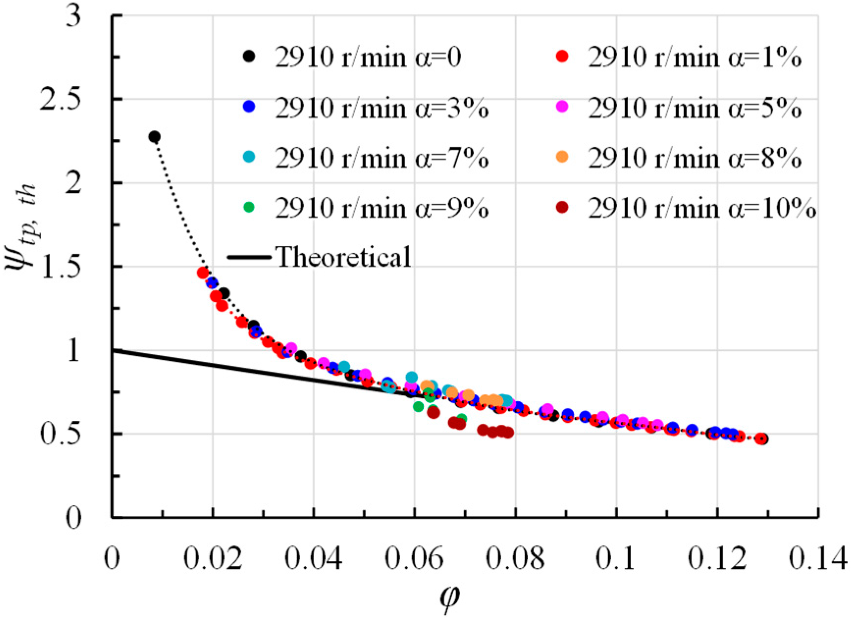
6.1. Pump Head Deterioration Ratio ψ*: Comparisons between Experiments and One-Dimensional Two-Phase Flow Model

Results deduced from Minemura’s model [4] are first compared with experimental ones. They correspond to the solid lines plotted in Figure 8a–c. Up to a = 6%, they all give the same performance deterioration ratio as the model used by Tomiyama et al. [19] (see upper solid black curve) and Hench [20] (see lower solid black curve) for all of the flow coefficients at nominal speed (2910 r/min), and the two highest ones for 2300 r/min. The drag coefficient in Equation (2) is also used in the 3D-URANS numerical simulation. Finally, for the smallest rotational speed and flow coefficient values (φ = 0.038), the evolution of ψ* looks quite similar to the lower solid black curve (Figure 8c) corresponding to the churn flow regime used for the drag coefficient proposed by Zuber and Hench [21], the value of which depends on the bubble diameter and local void fraction. Since all of the experimental results regarding the pump deterioration ratio are located between these two curves, thus, it is believed that the complete flow structure should be considered not only inside the impeller, but also at the pump inlet section. Possible combinations of bubble and churn flow may arise due to the internal three-dimensional flow structure and void fraction inside the impeller [22]. In addition, it may arise when the flow rate and/or rotational speed are too low, including inlet recirculation. This was obviously not taken into consideration in previous studies when using a one-dimensional model. This is the reason why the URANS approach results are presented in the next section.

6.2. 3D-URANS Overall Performance Results

6.2.1. Comparison between the Initial and Modified Turbulence Model (See Section 3.3)

For pure water (Figure 9) and different inlet void fraction conditions (Figure 10a–d), comparisons of overall pump performance between experiments and 3D-URANS results are presented. For numerical and experimental comparisons on pump overall performance, the final mesh of 2,775,915 elements can be considered quite good (Figure 9) for a wide range of flow coefficients. A small shift in the flow coefficient can be seen probably due to some flow leakage during the experiments.

When using the modified turbulence model, the numerical results show a better overall performance of the pump than the initial model, especially for low flow coefficients, as shown in Figure 10a,b with quite lower scattering between the experiments and the 3D-URANS calculation. Consequently, the efficiency curves are quite similar to the experimental curves (Figure 10c,d).

6.2.2. 3D-URANS Results Comparison for Different Inlet Void Fraction and Flow Coefficients

These results are also plotted in Figure 8a–c, using green symbols for comparisons with experimental ones. Compared with the one-dimensional models already presented in the previous section, the calculation results give slightly better results when the values of a increase up to 7% at the rated rotational speed. The effects of rotational speed are not well predicted, which are probably for the same reasons that have been highlighted previously.

Some additional effects must be taken into consideration when the flow coefficient is more reduced, such as for example pressure level effects on bubble diameter, which is not discussed in the present work. Concerning this particular point, one has shown that the main loss coming from the two-phase flow character appears in the first 20% of the blade passage, where the pressure increase is generally low. There is probably an effect when the rotational speed is decreasing, but it has not been evaluated in the present analysis.

6.3. Local Impeller Passage Flow Structures

6.3.1. Flow at Inlet Impeller Section

A particular focus on inlet flow conditions is shown in Figure 11 for low flow rates in order to illustrate the effects of a. Strong reverse inlet pre-rotation flow with high tangential absolute velocities can be seen for pure water. When a = 7%, the flow pattern strongly changed at the pump inlet tube section; recirculation does not exist anymore, or is quite small. This is because air is going toward the pipe external radius due to the lower air velocities and the axial adverse pressure gradient along the streamline paths. Consequently, the reverse flow mainly takes place inside the first part of the impeller channel. This may explain what has been experimentally observed when a rapid breakdown of the pump occurs.

The following pictures in Figure 12 describe for a constant value of a = 7%, the evolution of the surfaces of the constant local void fraction α = 15% for two different water flow rates. Although interpretation difficulties arise in such complicated flow patterns, one can detect the air–water mixture locations at the upstream inlet bend of the impeller hub, and the shroud sections inside the regions indicated by red color areas. The more the flow rate decreases, the more it spreads and tends to block the inlet shroud region. This is the reason why the local void fraction appears partly on the suction side of the blade’s leading edge, and not close to the shroud, but rather in the second part of the suction side toward the mid-height and the hub. When the flow rate decreases, because of a higher inlet incidence angle, the void fraction extends to the entire suction-side blade height. At the impeller inlet section, more flow blockage can be seen; this may explain why no water inlet recirculation occurs when the inlet void fraction is important, as already discussed earlier. Further downstream, this void fraction value extends toward the mid-impeller channel (green color circles). For Q = 30 m³/h, a separation zone can be seen starting from the pressure side of the hub region, which migrates toward the mid-impeller passage as well. As pointed by Gülich [1], such a complicated flow pattern results from the dominant body forces and inertia for the liquid behavior (due to the density ratio between water and gas), while gas distribution is mainly determined by the pressure field and secondary flows. In the next section, the void fraction on the pressure and suction sides of the impeller is going to be analyzed more specifically.

6.3.2. Flow inside the Impeller Section

Void fraction distributions for decreasing flow rate values on the impeller blade and at the outlet radius of the impeller are shown in Figure 13a–d. Looking at the leading-edge regions of the impeller, a high local void fraction (between 20–30%) appears on the suction side mainly close to the shroud. High α values (up to 100%, corresponding to full air) appear on the pressure side of the shroud corner for Q = 30 m³/h, just after the inlet throat section of the impeller passage. The corresponding drag force, acting on a bubble, combined with the adverse pressure gradient inside the impeller passage, forces the gas bubble to move toward the pressure side where the local liquid relative velocity tends to be lower.

For a flow rate of 40 m³/h, the local void fraction values remain relatively small at both sides of the impeller leading edge. This is perhaps the reason why the experimental results show that the pump is still working at a high inlet a (up to 10%; see Figure 2) without gas locking. Finally, for 20 m³/h, a quite high local void fraction can be seen on the suction side of the leading edge due to incidence angle effects (see again Figure 11b for the meridional plane).

Further downstream, and for all of the flow rates, high void fractions are located near the pressure side, close to the second throat. This has been already mentioned by Mirakami and Minemura [3]. This is attributed to the increase in the velocity difference between the water and the gas when the void fraction increases. The corresponding drag force, acting on a bubble, combined with the adverse pressure gradient inside the impeller passage, forces the gas bubble to move toward the pressure side where the local liquid relative velocity tends to be lower. As an example, this is clearly obtained by the CFD results given in Figure 14 for the mid-section between the hub and the shroud, for Q = 30 m³/h.

By looking at the additional maps for the specific local void distribution (Figure 15), we can have a better insight on the pressure and suction sides of the blade. For instance, at a given flow rate (Q = 30 m³/h), it can be observed that on the pressure sides, the pattern of air bubbles differs between a = 5–7%. For a = 5%, high values of local void fraction are reached and spread along the blade height just after the leading edge. Then, due to the Coriolis force, the liquid is mainly present on this pressure side, and finally, due to the radial pressure gradient and slip velocity, air accumulates again close to the trailing edge. When a increases to 7%, air locations are shifted downstream in the hub region, and the liquid (and low local void fractions) area takes a larger surface and pushes air closer to the outlet blade section. As already mentioned, this last case exhibits strong 3D effects with flow separations and reverse flow regions.

One can observe that the more the flow rate decreases, the more of high void fractions are shifted toward the pressure side due to the decrease of the mean relative velocities. For Q = 20 m³/h, all of the passages are filled with air. All of the blade passages do not have the same pattern due to the presence of the volute tongue.

At the impeller outlet plane, the void fraction does not exceed 30%, instead of reaching the lowest flow rate, for which the values may reach up to 60%. Just downstream of the impeller, due to strong mixing, the void fraction strongly decreases (not shown here). Close to nominal conditions, the void fraction values obtained from CFD are quite similar to the values predicted by the model developed by Minemura et al. [3]. On the pressure side, there is always a thin layer that develops with high void fraction values.

The next set of figures gives the pattern of the local void fraction in the mid-section plane between the hub and the shroud, for decreasing flow rates and a given a value of 7%. This corresponds to the maps given in Figure 16.

All of the flow patterns that have been found and described inside the impeller channels are the consequences of what happens at the impeller inlet section just before and after the blade leading-edge area. This means that one has to find the local design modifications forcing high two-phase flow values to be mixed with the main flow using additional local body forces. For this reason, it is expected that the blade clearance between the hub and the shroud can be an efficient way to create a local vortex for a better mixing, avoiding a local accumulation of the high void fraction values on the meridional plane inlet sections and in the blade-to-blade plane further downstream of the inlet passage throat. This will be carried out in a future work.

7. Conclusions

Experimental and numerical analysis has been performed in a centrifugal pump for different flow coefficients and inlet void fractions up to 10%. The effect of rotational speed has also been investigated. The main conclusions are the following:

• Pump performance degradation is more pronounced for low flow rates compared to high flow rates when the inlet void fraction increases. The starting point of a severe pump degradation rate is related to a specific flow coefficient, whose value corresponds to the change of the slope of the theoretical head curve. When increasing the inlet void fraction, the degradation slope curves increase (with a negative sign) with the decreasing flow coefficient. The more the rotational speed decreases, the more the experimental pump performance is affected at a given inlet void fraction value.
• Existing one-dimensional models can be considered quite good tools for the first step of a two-phase flow analysis. They give good global indications based on the mean values along one streamline, but attention should be taken when using non-dimensional flow coefficients. The chosen particle fluid model with interface transfer terms looks quite suitable for evaluating pump performance degradation up to an a value of 7%.
• For a higher a value, CFD can’t always correctly predict the sudden breakdown of the pump performance as obtained by measurements. This is probably due to the flow regime inside the impeller, which does not correspond to a bubbly one anymore. However, for the lowest flow rate, the performance breakdown is well predicted with the modified turbulence model.
• The difference between experimental and numerical results exist not because of rotational speed, but because of its consequence on the local velocity values that decrease according to the flow coefficient, and more specifically at the pump inlet tube and at the pump inlet section. Numerical simulations must take churn flow characteristics into account in order to get better results. Both bubbly and churn flow conditions may be present for inlet flow conditions depending on the experimental setup, rotational speed, and the pump flow coefficient, even at nominal conditions.
• The numerical simulation gives interesting local flow information that would be taken into consideration for new design approaches at the pump inlet section for an improved two-phase flow suction capability of centrifugal pumps.

References

1. Gülich, J.F. Centrifugal Pumps; Springer: Berlin/Heidelberg, Germany; New York, NY, USA, 2010; ISBN 978-3-642-12823-3. [Google Scholar]
2. Mikielewicz, J.; Wilson, D.G.; Chan, T.C.; Goldfinch, A.L. A method for correlating the characteristics of centrifugal pumps in two-phase flow. J. Fluids Eng. 1978, 100, 395–409. [Google Scholar] [CrossRef]
3. Murakami, M.; Minemura, K. Effects of entrained air on the performance of a centrifugal pump First report- Performance and Flow Conditions. Bull. JSME 1974, 17, 1047–1055. [Google Scholar] [CrossRef]
4. Minemura, K.; Uchiyama, T.; Shoda, S.; Egashira, K. Prediction of air-water two-phase flow performance of a centrifugal pump based on one-dimensional two-fluid model. J. Fluids Eng. 1998, 120, 237–334. [Google Scholar] [CrossRef]
5. Si, Q.R.; Cui, Q.L.; Zhang, K.Y.; Yuan, J.P.; Bois, G. Investigation on centrifugal pump performance degradation under air-water inlet two-phase flow conditions. La Houille Blanche 2018, 3, 41–48. [Google Scholar] [CrossRef]
6. Secoguchi, N.; Takada, S.; Kanemori, Y. Study of air-water two-phase centrifugal pump by means of electric resistivity probe technique for void fraction measurement-First report-measurement of void fraction distribution in a radial flow impeller. Bull. JSME 1984, 27, 931–939. [Google Scholar] [CrossRef]
7. Estevam, V.; França, F.A.; Alhanati, F.J. Mapping the performance of centrifugal pumps under two-phase conditions. In Proceedings of the 17th International Congress of Mechanical Engineering, Sao Paulo, Brazil, 10–14 November 2003. [Google Scholar]
8. Barrios, L.; Prado, M.G. Experimental visualization of two-phase flow inside an electrical submersible pump stage. J. Energy Resour. Technol. 2011, 133. [Google Scholar] [CrossRef]
9. Müller, T.; Limbach, P.; Skoda, R. Numerical 3D RANS simulation of gas-liquid flow in a centrifugal pump with an Euler-Euler two-phase model and a dispersed phase distribution. In Proceedings of the 11th European Conference on Turbomachinery, Fuild Dynamics and Thermodynamics, Madrid, Spain, 23–25 March 2015. [Google Scholar]
10. Suryawijaya, P.; Kosyna, G. Unsteady measurement of static pressure on the impeller blade surfaces and optical observation on centrifugal pumps under varying liquid/gas two-phase flow condition. J. Comput. Appl. Mech. 2001, 6759, D9–D18. [Google Scholar]
11. Si, Q.R.; Bois, G.; Zhang, K.Y.; Yuan, J.P. Air-water two-phase flow experimental and numerical analysis in a centrifugal pump. In Proceedings of the 12th European Conference on Turbomachinery, Fluid Dynamics and Thermodynamics, Stockholm, Sweden, 3–7 April 2017. [Google Scholar]
12. Yakhot, V.; Orszag, S.; Thangam, S.; Gatski, T.; Speziale, C. Development of turbulence models for shear flows by a double expansion technique. Phys. Fluids A Fluid Dyn. 1992, 4, 1510–1520. [Google Scholar] [CrossRef] [Green Version]
13. Clift, R.; Grace, J.; Weber, M. Bubbles, Drops and Particles; Academic Press: New York, NY, USA, 1978. [Google Scholar]
14. Wang, J.; Wang, Y.; Liu, H.; Huang, H.; Jiang, L. An improved turbulence model for predicting unsteady cavitating flows in centrifugal pump. Int. J. Numer. Methods Heat Fluid Flow 2015, 25, 1198–1213. [Google Scholar] [CrossRef]
15. Dular, M.; Coutier-Delgosha, O. Numerical modelling of cavitation erosion. Int. J. Numer. Methods Fluids 2009, 61, 1388–1410. [Google Scholar] [CrossRef]
16. Coutier-Delgosha, O.; Fortes-Patella, R.; Reboud, J.L. Evaluation of the turbulence model influence on the numerical simulations of unsteady cavitation. ASME J. Fluids Eng. 2003, 125, 38–45. [Google Scholar] [CrossRef]
17. Schäfer, T.; Bieberle, A.; Neumann, M.; Hampel, U. Application of gamma-ray computed tomography for the analysis of gas holdup distributions in centrifugal pumps. Flow Meas. Instrum. 2015, 46, 262–267. [Google Scholar] [CrossRef]
18. Baker, O. Simultaneous Flow of Oil and Gas. Oil Gas J. 1954, 53, 185–190. [Google Scholar]
19. Tomiyama, A.; Kataoka, I.; Sakaguchi, T. Drag coefficients of bubbles. 1st report. drag coefficients of a single bubble in a stagnant liquid. Nihon Kikai Gakkai Ronbunshu B Hen/Trans. Japan Soc. Mech. Eng. Part B 1995, 61, 2357–2364. [Google Scholar]
20. Hench, J.E.; Johnston, J.P. Two-dimensional diffuser performance with subsonic, two-phase, air-water flow. ASME J. Basic Eng. 1972, 107, 105–121. [Google Scholar] [CrossRef]
21. Zuber, N.; Hench, J.E. Steady State and Transient Void Fraction of Bubbling Systems and Their Operating Limits; General Electric: Schenectady, NY, USA, 1962. [Google Scholar]
22. Zhu, J.J.; Zhang, H.Q. A review of experiments and modeling of gas-liquid flow in electrical submersible pumps. Energies 2018, 11, 180. [Google Scholar] [CrossRef]
Figure 1. Test rig.
Energies 11 03048 g001
Figure 2. Sensor locations.
Energies 11 03048 g002
Figure 3. Three-dimensional (3D) numerical domain (partial) with local meshing.
Energies 11 03048 g003
Figure 4. Grid independence results.
Energies 11 03048 g004
Figure 5. The law of the f(ρm) with the density in the mixed phase.
Energies 11 03048 g005
Figure 6. Head coefficient at n = 2910 r/min.
Energies 11 03048 g006
Figure 7. Theoretical head coefficient.
Energies 11 03048 g007
Figure 8. Pump degradation level for three flow coefficients. Comparison between experiments, one-dimensional (1D) model and “Three-Dimensional Unsteady Reynolds Average Navier–Stokes” (3D-URANS) calculations. Solid black lines represent the theoretical evolution from Minemura’s approach using two different bubble drag coefficients (upper line for bubbly flow, lower line for churn flow): (a) φ = 0.077; (b) φ = 0.058; (c) φ = 0.038.
Energies 11 03048 g008
Figure 9. Comparison between experiment and numerical head and efficiency (a = 0).
Energies 11 03048 g009
Figure 10. Comparison between experiment and numerical head coefficient and efficiency for four different a values: (a) Head coefficients when a = 3%; (b) Head coefficients when a = 5%; (c) Efficiency when a = 3%; (d) Efficiency when a = 5%.
Energies 11 03048 g010
Figure 11. Local two-phase flow pattern inside the impeller passage (not including impeller wall regions), nominal rotational speed, φ = 0.038: (a) a = 0% (b) a = 7%; (c) a = 0%; (d) a = 7%.
Energies 11 03048 g011
Figure 12. Constant void fraction iso-lines inside the impeller passage when a = 7%: (a) φ = 0.077; (b) φ = 0.058.
Energies 11 03048 g012
Figure 13. Void fraction pattern at the impeller outlet section, a = 7%: (a) φ = 0.077; (b) φ = 0.058; (c) φ = 0.038.
Energies 11 03048 g013
Figure 14. Void fraction pattern in the blade-to-blade mid-section plane, Q = 30 m3/h, φ = 0.058: (a) a = 3%; (b) a = 5%; (c) a = 7%.
Energies 11 03048 g014
Figure 15. Void fraction pattern on the blade surface, φ = 0.058: (a) a = 3%; (b) a = 5%; (c) a = 7%.
Energies 11 03048 g015
Figure 16. Void fraction pattern in the blade-to-blade mid-section plane for different flow rates, a = 7%: (a) φ = 0.077; (b) φ = 0.058; (c) φ = 0.038.
Energies 11 03048 g016