Numerical Investigation on the Influence of Areal Flow on EGS Thermal Exploitation Based on the 3-D T-H Single Fracture Model

1
School of Civil Engineering and Architecture, Nanchang University, Nanchang 330033, China
2
State Key Laboratory of Geomechanics and Geotechnical Engineering, Institute of Rock and Soil Mechanics, Chinese Academy of Sciences, Wuhan 430071, Hubei, China
*
Author to whom correspondence should be addressed.
Energies 2018, 11(11), 3026; https://doi.org/10.3390/en11113026
Submission received: 17 September 2018
/
Revised: 22 October 2018
/
Accepted: 24 October 2018
/
Published: 4 November 2018
(This article belongs to the Special Issue New Stimulation Methods for Recovery of Energy and Minerals from Ultra-low-permeability Rock Formations)
Abstract
:The research on the factors of heat recovery performance of Enhanced Geothermal Systems (EGS) is an important issue, especially in the well position optimization in EGS, because it can maximize the economic benefits of EGS. Based on the three-dimensional thermo and hydro (TH) single-fracture model, a flow field in the EGS is added to the model, the thermal energy mining of the EGS thermal reservoir is realized through the double well and better study of the impact of regional flow on EGS well placement. To verify the reliability of the three-dimensional numerical model, the comparison between the two-dimensional single fracture model and the single fracture analytical model is performed under the same conditions, and it is found that there is a good agreement between the numerical and the analytical solutions. The influence of the direction of regional flow on the thermal recovery performance of EGS is studied, and the operating lifetime, power generation and heat production rate of the system are used as the evaluation indicators. It is found that there are two stagnation points in the flow field under regional flow conditions, and the stagnation point position changes regularly with regional flow direction. The direction of regional flow has a great influence on the heat extraction ratio and service lifetime of the geothermal system, the layout of the double well must take into account the regional flow. When only considered the influence of regional flow on EGS, after 50 years of EGS operation, the production well temperature and system operating lifetime increase with the increase of β (the angle between the direction of the regional flow and the line connecting the centers of the two wells). When it has regional flow, the greater the well spacing, the greater the temperature of the production well, but when the well spacing increases to a certain value, the well spacing will not affect the temperature of the production well.
1. Introduction
Geothermal energy is an alternative, clean and renewable energy. Geothermal energy is stable and does not depend on weather conditions, making it therefore superior to wind, solar and tidal power. As a result, geothermal energy has been widely used in electricity generation in many countries. The Enhanced Geothermal Systems (EGS) is a well-known method of geothermal mining based on the development of dry hot rock [1].
The concept of EGS, which includes the earlier concept of Hot Dry Rock (HDR), originated at the Los Alamos National Laboratory (LANL) in the USA [2]. The principle is that direct wells or directional wells are drilled in target areas of dry hot rock as injection wells and production wells, and by hydraulic fracturing, the natural cracks are opened and expanded, and the main artificial fractures are produced between the upper injection and the low-yielding well. During production, water is pumped from the injection well to a certain flow rate and temperature, the water flows along the fracture while absorbing the heat from the surrounding rock. Finally, a high-temperature and high-pressure water or a water vapor mixture is extracted from the production well, which is then used comprehensively for applications such as power generation and heating. Low temperature water passes through the energy conversion station, and is then pumped back into the underground from the injection well. This pattern of development and utilization is the enhanced geothermal system (Figure 1).
At present, numerical simulation is the main tool used to study the EGS system [3]. In recent years, in order to simulate the geothermal mining process, a large number of open source and commercial software packages have emerged. To list a few here, TOUGH2 (from the Lawrence Berkeley National Laboratory) [4] uses the finite difference method (FDM), while the Multi-physical Field Numerical Computing Platform by COMSOL [5] and FEHM (Los Alamos National Laboratory) [6] are based on the finite element method (FEM), ECLIPSE (Schlumberger) [7] and Fluent (ANSYS) [8] use the finite volume method (FVM). Table 1 gives a brief introduction to the above software. They have all been successfully used to simulate the thermal extraction of EGS reservoirs using complex geometries [6,8,9,10,11,12,13,14,15,16]. Other than that, Ghassemi et al. [17], and the Kumar and Gutierrez [18] predictive three-dimensional effect used the Bem method (BEM). Safari and Ghassemi [19] using the displacement discontinuous element method (DDM) to study the influence of permeability on the permeability of the produced EGS, McClure and Horne [20] applied the DDM method to simulate the heat transfer and mass transfer problem of discrete fracture networks.
There are many factors affecting the thermal recovery of EGS, such as injection flow, reservoir permeability, well spacing and regional flow, etc. [21,22,23,24,25,26]. In order to maximize the benefits of EGS thermal mining, Biagi et al. [11] used a multi-objective genetic algorithm, and Juliusson et al. [22] used the fmincon function in MATLAB to study the effect of injection flow and get the optimal solution. Ghazal et al. [23] found that the higher the reservoir permeability, the smaller the flow resistance of the fluid in the reservoir, resulting in higher flow rates and higher heat recovery rates. Jing et al. [24,25] found that the greater the distance between the injection well and the production well, the longer the thermal breakthrough time, which is beneficial to long-term thermal exploitation. However, the larger well spacing requires a larger pressure difference, not fully utilizing the heat of the reservoir. Ekneligoda et al. [26] found that the optimal well spacing under specific conditions was 600 m by comparing the temperature distribution in the reservoir. The total amount of groundwater (water below the surface) is about 8 × 10⁶ km3, of which about 50% is distributed in the depth range of about 800 m below the ground [27]. This shows that the underground regional flow is widespread. Gringarten and Sauty [28] used theoretical research methods to study the thermal energy extraction of geothermal systems with uniform regional flow, but Schulz [21] found that this calculation method is too cumbersome and inefficient. Rodemann [29], Heuer [30], and Wu et al. [31] studied dual wells and multi-well systems, but they did not consider the effects of regional flows. Wu et al. [32] used a theoretical research method to establish a two-dimensional semi-analytical model, they studied the influence of regional flow on geothermal system thermal mining, and studied well location optimization in the presence of regional flow in EGS reservoirs, but its application model is simple, it can’t better reflect the real complex reservoir situation.
In this paper, the thermal reservoir is considered to consist of porous media and a single fracture. The complete EGS double well numerical model is established by COMSOL Multiphysics 5.3a, adding a uniform regional flow to the model to study the impact of regional flow on EGS, the influence of the initial injection flow of the injection well and well spacing on the thermal recovery performance of EGS.
2. TH Coupled Single Fracture Model
2.1. The Governing Equation
2.1.1. Reservoir Flow Field Governing Equation
Fluid flow in porous media can be described with the following mass conservation expression:
where, ρ (kg/m3) indicates the density of water; εp indicates the porosity of reservoir; t (s) indicates the time; and u (m/s) indicates the velocity. According to the Darcy’s law, u is described by the following momentum equation:
where, κ (m2) indicates the permeability of reservoir; μ (Pa·s) indicates the viscosity of water; p indicates the pressure; ρg∇z indicates the gravity term, and z indicates the direction of vertical.
The mass conservation equation for a single fracture is written as:
where, df (m) indicates the aperture of fracture; ∇T indicates the gradient operator restricted to the fracture’s tangential plane; εf indicates the porosity fracture; uf indicates the velocity of Darcy in the fracture, which is also described by Darcy’s law:
where, κf (m2) indicates the fracture permeability. Qm in Equations (1) and (3) represents the mass transfer between the porous media and fractures.
2.1.2. Reservoir Temperature Field Governing Equation
Between the fluid and the bedrock, the heat transfer is usually described by the local heat balance equation [33]. This means that the temperature of the fluid in the bedrock is the same as that of the rock. The following energy conservation equations are used to describe the heat transfer process in porous media:
of which:
where, T (K) indicates the temperature of the porous media; θp represents the volume fraction of the porous medium; kp indicates the thermal conductivity of porous media; cp.p indicates the Specific heat capacity of porous media; Cp (J/(kg·K)) indicates the heat capacity of the fluid; (ρcp)eff and keff are the effective volumetric capacity and effective thermal conductivity, respectively. Under high temperature conditions, the physical properties of water vary with the temperature, thus the water density ρ (kg/m3) and viscosity μ (Pa·s) are described based on [34] as a function temperature with:
where Tc (°C) indicates the temperature in degrees Celsius and T (K) represents the temperature in Kelvin.
The heat transfer equilibrium equation of a fracture is given as:
of which:
where, θfr is the volume fraction of fracture boundary material; kfr is the thermal conductivity of fracture; ρfr is the fracture density; cp.fr is the specific heat capacity of the fracture; dfr is the fracture width; Qf,r indicates the heat transfer between the porous media and fractures, which results from the fluid transport and heat conduction.
2.2. Model Verification
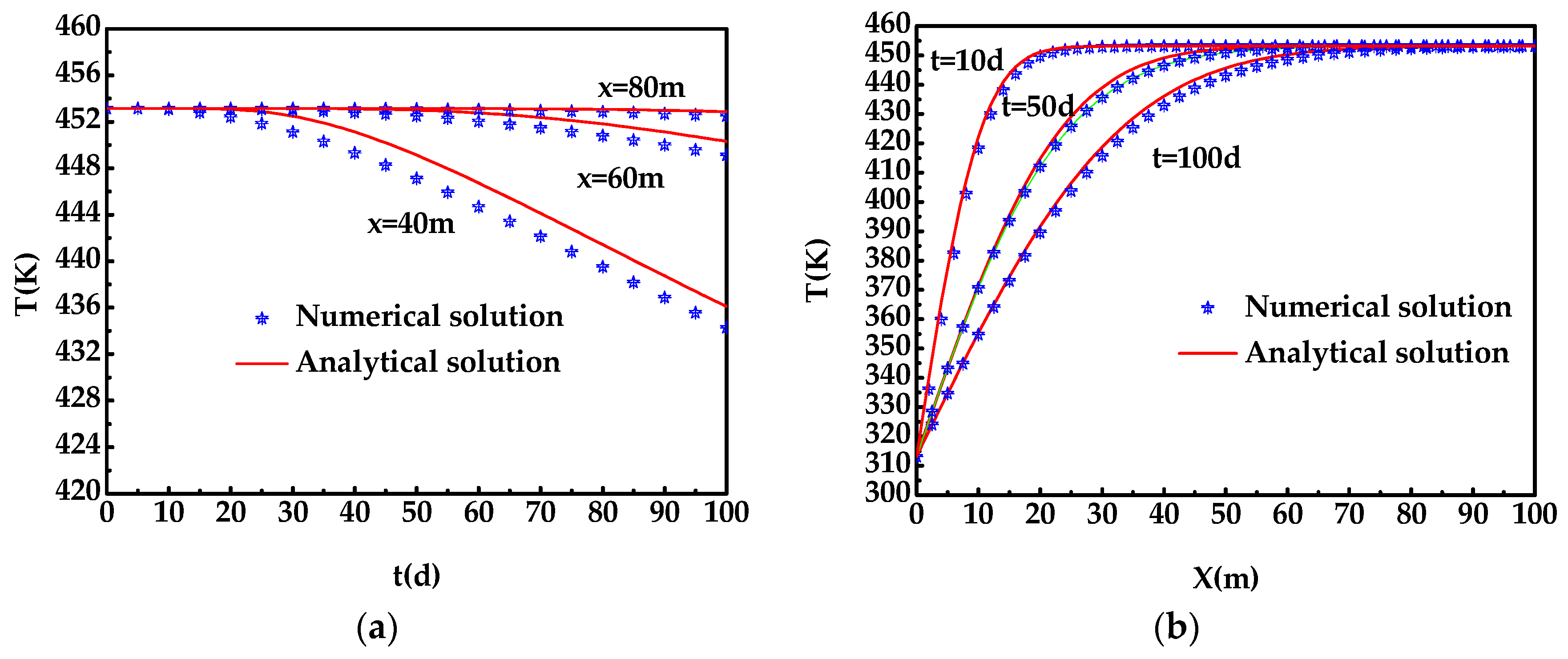
The above control equation and the corresponding initial and boundary conditions constitute the mathematical model and definite solution conditions of fluid flow and heat transfer in the EGS reservoir. The biggest advantage of the finite element software COMSOL is to solve the partial differential equations of the model. Before the study, we must verify the reliability of our model. Here, the numerical model is verified by an analytical solution to the heat transfer problem of water rock flow under a simple heat flow coupling [35,36]. As shown in Figure 2, the rock matrix is divided into two parts by a horizontal fracture. Assume the initial temperature of the rock matrix is Tr0, the fracture width is δ, the length is L, the thermal conductivity of rock matrix is kr, the fracture fluid density is ρf, the density of rock matrix is ρr, the specific heat capacity of fracture fluid is cf, the heat capacity of rock matrix is cr, and the initial water injection temperature is Tf0. The fluid flows into the fissure at a constant velocity uf, and exchanges heat with the high-temperature rock matrix on both sides during the flow through the fissure to solve the temperature change with time at different positions of the fissure. Set the two-dimensional coordinate x-y axis, the fluid inlet is the coordinate origin, the direction of the x-axis is along the direction of fluid flow, and the direction is positive to the right. The y-axis is perpendicular to the x-axis and the upward direction is the positive direction. Hu [37] gave the following analytical solution to this problem:
A rectangular matrix of 100 m × 100 m is constructed to characterize the rock matrix of the single fracture model. The values of the parameters are shown in Table 2. Figure 3a shows the temperature variation with time at three different positions (i.e., x = 40 m, 60 m, and 80 m) in the fracture; while Figure 3b indicates the temperature distribution along the fracture at various times (i.e., t = 10 d, 50 d, and 100 d, where unit d represents the time of day). It can be seen from Figure 3 that there is a good agreement between the numerical solution and the analytical solution, and there is only a slight error. There are two reasons for this subtle error. One is the discrete error of the numerical model. Secondly, the computational region of the analytical solution hypothesis is semi-infinite, and the computational region of the numerical model is a finite square region of 100 m × 100 m. Thus, it is proved that the calculation of the heat-water coupling process using the COMSOL numerical model is reliable.
2.3. Model Establishment of Enhanced Geothermal System
Fissured rock masses are a kind of complex engineering medium, which is wide spread in slopes and underground caverns, such as in the fields of energy, transportation, mining and hydraulic engineering [38,39,40]. The EGS reservoir rock mass with good open fractures has been successfully reformed by hydraulic fracturing, which must be considered in the numerical simulation. At present, the equivalent method is used for the fractured rock mass with dense fracture distribution, which is generally simplified by the continuum theory, and the discrete model is often used to solve large faults or fractures with major penetration [41]. It has also been shown that in some cases, most of the heat transfer fluid in the EGS may be transferred directly from the injection well to the production well through one or several major flow channels [42].
This study establishes a single fracture model of ideal double well for EGS thermal mining; the reservoir fracture network is equivalent to a horizontal single fracture, as shown in Figure 1. Assume that the thermal reservoir is a cube with a side length of 500 m, the x-axis is parallel to the line formed by the center of the two wells, the z-axis is parallel to the axis of the well, and the y-axis is perpendicular to the x-axes and z-axes. A horizontal fracture with a width of 0.002 m is set at the position of z = 250 m. In this paper, a regional flow with a hydraulic gradient of 0.01 [m/m] is set in the fracture. The coordinates of the center of the injection well are (350, 250, z), the coordinates of the center of the production well are (150, 250, z), and the length of the injection well and the production well is 500 m. The model is solved by commercial finite element software COMSOL Multiphysics, Figure 4 shows the finite element model in the computational process of this paper.
Here we will select the Darcy’s law module in the fluid module and the porous medium heat transfer module in the heat transfer module. The diameter of both the production well and the injection well is 0.4 m. The corresponding finite element model contains 73,913 tetrahedral elements, which is shown in Figure 4. Material parameters are shown in Table 3.
2.4. Initial and Boundary Conditions
On the basis of the above model, the whole process of EGS development process from water injection to production process is simulated. Boundary conditions and initial conditions are as follows:
(1) Initial and boundary conditions of the flow field
The upper and lower sides of the EGS model are impervious to water. A uniform regional flow parallel to the x-y plane with a hydraulic gradient of 0.01 [m/m] is set. It is assumed that the water loss is not considered between the injection well and the mining well, so the flow rate of the injection well is equal to that of the mining well.
(2) Temperature field initial and boundary conditions
Assume that the temperature of the injection well is consistent with the water temperature in the well, which is 293.15 K (20 °C), the initial surface temperature of the model is 493.15 K (220 °C), and the geothermal gradient is increasing along the z-axis direction with a gradient of 0.04 [°C/m]. The average water temperature of the production well is used as the heat extraction temperature of the EGS. The upper and lower sides of the model are heat insulation surfaces, while the other surfaces can exchange heat with the outside.
2.5. Thermal Recovery Evaluation System
In the numerical simulation of enhanced geothermal system, it is necessary to quantitatively find out the influence of various influencing factors on the heating performance and heat recovery rate of EGS through some indicators [43]. According to Chen and Jiang [44], Zhang et al. [45], Yuan et al. [46], Gao [47], it is found that the commonly used EGS thermal performance evaluation indicators are:
- (1)
- Operating lifetime of EGS: the total operating time of the system from the initial operating temperature of the thermal fluid in the production well in EGS to below 150 °C.
- (2)
- Heat production rate of EGS:where: Q (Kg/s) is the fluid mass flow rate; Cρ (J/(kg·°C)) is the specific heat capacity of the fluid; T(t) is the temperature of the heat generating fluid at time t; Tin (°C) is the initial fluid injection temperature.
- (3)
- Overall thermal recovery rate R(t) refers to the ratio of the heat energy extracted after the operating time of the system t to the total recoverable heat energy in the reservoir:where: Tr (°C) is the initial rock temperature; V (m3) is the reservoir volume; ε is the porosity of the reservoir; The denominator represents the total recoverable amount of the reservoir and the numerator represents the heat energy that has been extracted after the system running time t.
- (4)
- The local thermal recovery rate RL refers to the ratio of the thermal energy extracted from the local location of the reservoir to the total recoverable energy after the system operation time t:where: Tr(t) is the rock temperature at time t, °C.
- (5)
- Net power generation:where: ζ is the conversion coefficient between thermal energy and electrical energy, the article takes 0.45; T0 is the minimum conversion temperature, the article assumes that it can reach 293.15 K (20 °C).
3. Influence of Regional Flow on EGS Thermal Mining Process
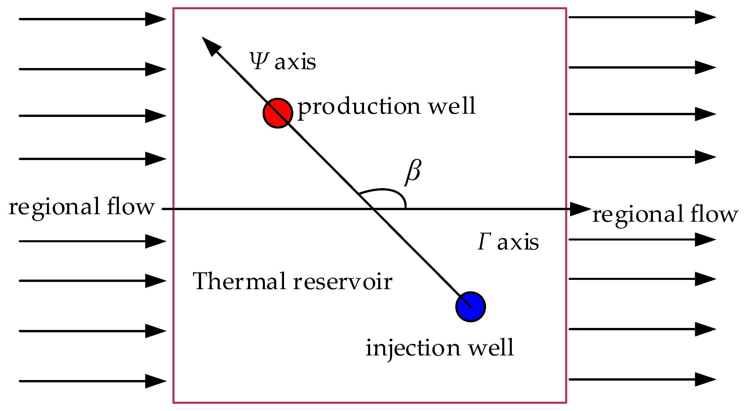
First, this paper considers the influence of regional flow on EGS thermal mining process. As shown in Figure 5, the angle between the direction of the regional flow and the line connecting the centers of the two wells is β. The S line connecting the centers of the two wells is the Ψ axis; the direction is from the injection well to the production well. The direction of the flow is The Γ axis, the Γ axis rotates counterclockwise to the Ψ axis angle is β (0° ≤ β ≤ 180°), the thermal recovery performance of EGS when the β angle is 0°, 45°, 90°, 135°, 180°, respectively analyze the effect of regional flow direction on the thermal mining process. In this paper, the initial conditions for this paper are an injection flow rate of 0.04 m3/s and a well spacing of 200 m, study the influence of different β values on the thermal recovery performance of EGS.
3.1. Influence of Regional Flow on EGS Fluid Field
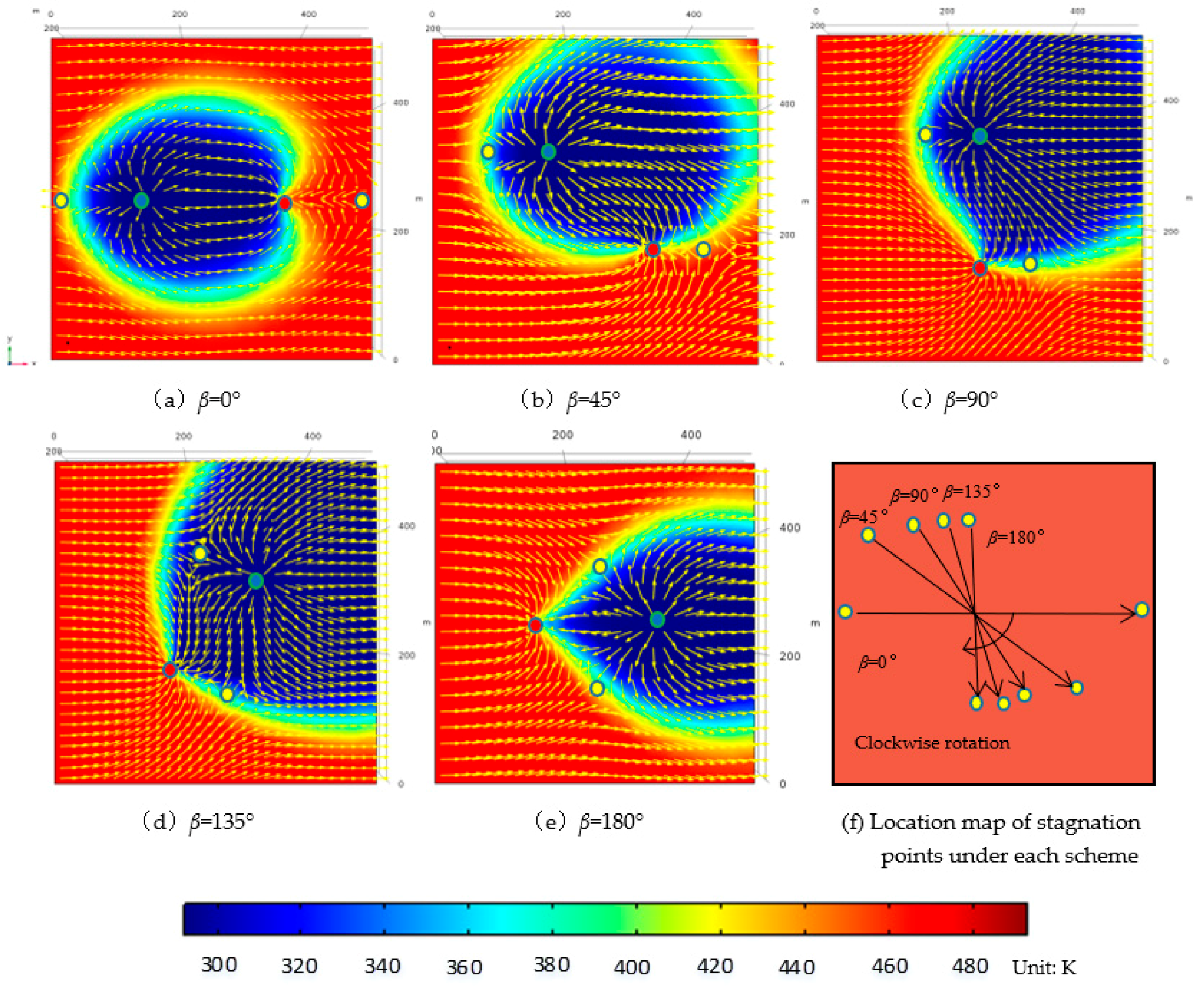
The flow behavior of the fluid in the EGS becomes more complicated when there is an areal flow. Figure 6 shows a vector diagram of the fluid flow of the EGS at different β values after 50 years. Figure 7 shows a streamlined graph of fracture at different β values after 50 years. As can be seen from Figure 6, there are two stagnation points for a double well EGS (the yellow circle is used to indicate the stagnation point in Figure 6). This is consistent with the conclusion of Wu [24] that uses the mathematical method of a semi-analytical solution, which also explains the correctness of the model from the side.
It can be clearly seen from Figure 6 that the direction of the regional flow has a great influence on the flow behavior of the fluid. First, the EGS has two stagnation points under the regional flow. If the two stagnation points are connected into a line segment, the direction is starting from the stagnation point near the injection well and pointing to the other stagnation point as the positive direction. It can be found that as β increases, the line segment rotates clockwise with respect to the centroid of the region (as shown in Figure 6f). Secondly, under the influence of regional flow, the proportion of fluid flowing out of the injection well in the production well also changes as the direction of the regional flow changes. When β = 0°, the largest proportion of fluid flowing into the production well from the injection well. When β = 180°, the smallest proportion of fluid flowing into the production well from the injection well. The reason for this phenomenon is that there is viscous force in the flow of the fluid. When the fluid in the regional flow meets the fluid infiltrating into the rock matrix at a certain flow rate, it will change the direction of movement of part of the fluid. As a result, part of the fluid cannot reach the production well, and the injection fluid flowing into the production well decreases as the value of β increases, the lost fluid increases.
Combined with Figure 7, it can be found that the flow behavior of the fluid in the fracture is greatly affected by the direction of the regional flow. It can be seen that the ratio of the number of streamlines between the production well and the injection well to the total number of production wells decreases with β increases, which also confirms the results obtained in Figure 6.
3.2. Influence of Regional Flow on EGS Temperature Field
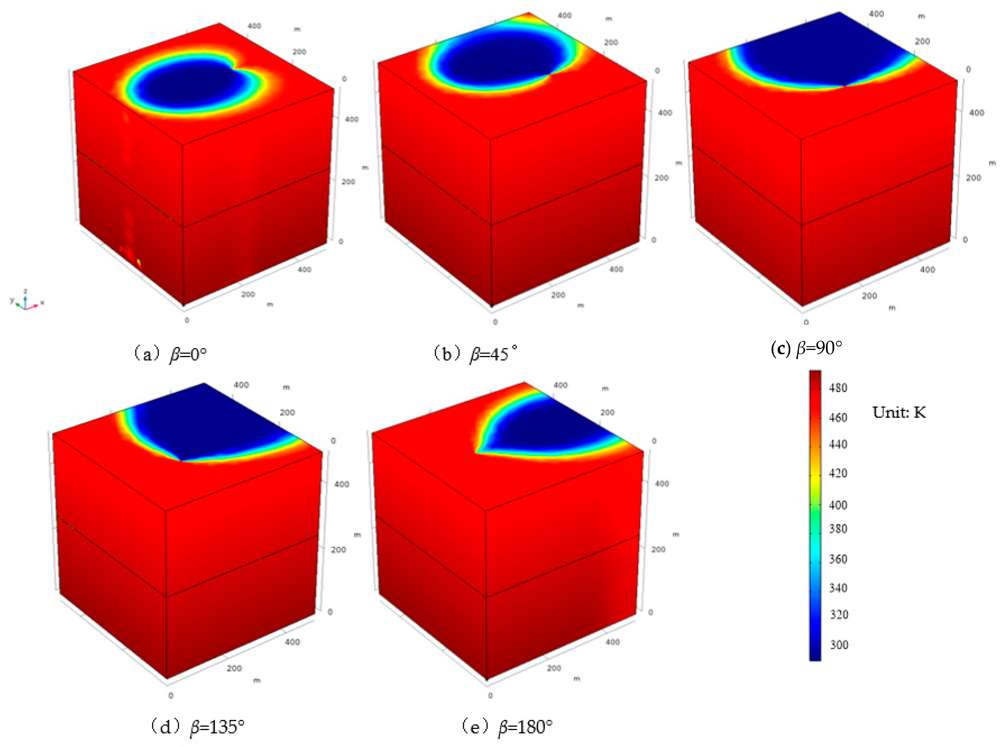
Figure 8 shows the temperature of EGS reservoirs change with different β after 50 years. It can be clearly seen from Figure 8 that after 50 years, the temperature field is mainly divided into three zones: the low temperature zone (shown in blue in Figure 8), the high temperature zone (shown in red in Figure 8) and the gradual zone (represented by the color of the other in Figure 8). For Figure 8a,b, the low temperature region is a closed ellipse, and the low temperature regions in Figure 8c–e are non-closed patterns. From Figure 8, it can be clearly seen that the proportion of the area occupied by the low temperature zone under different β is also different. In order to better study the influence of different β on the thermal recovery performance of EGS, the temperature curve of production wells with EGS under different β is given as shown in Figure 9.
Figure 9 shows the temperature profile of the production well over time for EGS at different β. It can be seen that the curve has two main phases: the steady phase and the falling phase. The output temperature of the production well remains constant during the steady phase, and it can be seen in the Figure 9 that the time of the stabilization phase increases with increasing β.
In the falling phase, the temperature of the production well decreases with time, and the rule can be obtained from Figure 9, it is that the downward trend of the curve in the descending phase gradually becomes slower as time goes by. The total operating time of the system from the initial operating temperature of the thermal fluid in the production well in EGS to below 150 °C (423.15 K). For the curve β = 0°, the EGS reaches its lifetime at the time of 13.99 years; when β = 45°, the system reaches the lifetime at the time of 18.75 years; while in other cases the EGS lifetime exceeds 50 years, for the actual development of the project is more reasonable. The smaller the β value, the smaller the temperature of the production well after 50 years, the faster the heat mining rate, but the shorter the service lifetime of the EGS; the larger the β value, the higher the temperature of the production well, the slower the heat mining rate, but the longer the service lifetime of the EGS. Therefore, a reasonable choice of β value has a significant impact on the thermal recovery performance of EGS.
3.3. Influence of Well Spacing on Thermal Performance of EGS
In this paper, five schemes with well spacing of 200 m, 250 m, 300 m, 350 m, and 400 m are investigated. Figure 10 shows the relationship between production well temperature and time under different β and well spacing conditions. Under the same β value, it can be found that within a certain range, the smaller the well spacing, the working fluid does not fully absorb the heat of the reservoir and reaches the production well, and the production well temperature is lower; If the spacing of wells is increased, the working fluid can fully absorb heat in a large area for a long time, and the production well temperature can also reach a high temperature (There are such relationships in Figure 10). However, it can be found from the Figure 10c–e that when the spacing of wells reaches a certain range, the fluid absorbs enough heat in the reservoir. When it does not reach the production well, it has reached the reservoir temperature and no heat is absorbed. At this point, increasing the spacing of wells has no significant influence on the temperature of mining heat, but it can make the operating lifetime of the system longer. However, too large spacing will increase the mining pressure. Therefore, the well spacing is important for the heating performance and needs to be determined after weighing the mining temperature and the recoverable time.
Comparing Figure 10a–e, it can be found that as the β value increases, the degree of dispersion between the curves of the corresponding graphs is larger, that is amplification of the effect of well spacing on the thermal recovery performance of EGS. This reason is caused by the fact that the areal flow affects the amount of fluid flowing from the injection well to the production well. With decreasing the β value, the proportion of fluid flowing into the production well from the injection well will decrease. By comparing the curves whose spacing is 200, 250, 300, 350 and 400 m, it can be found that the larger the spacing of wells is, the smaller the influence on the thermal exploitation performance of EGS is. This means that when the spacing of wells reaches a certain value, the regional flow has little influence on the thermal exploitation of EGS.
3.4. Effect of the Flow Rate on Output Temperature
Figure 11 shows the relationship of production well temperature over time at different initial injection flows. Here, the initial injection flow rate is set to 0.04 m3/s, 0.06 m3/s, 0.08 m3/s, and 0.1 m3/s, respectively. It can be found that as the initial flow rate Q increases, the temperature of the production well decreases (Figure 11b–e). The reason for this is that the flow rate of the fluid in the reservoir is accelerated due to the increase of the initial flow rate, which leads to the shorter travel time of the fluid to the production well and the shorter heat exchange time between the fluid and the thermal reservoir. It is worth mentioning that in Figure 11a, each curve has an intersection point at the time of 31.3 years.
Before 31.3 years, the temperature of the production well decreases with the increase of the initial injection flow rate, but the opposite result appeared after 31.3 years, comparing Figure 11a–e, the spacing between the curves was gradually increased from dense to discrete as the value of β increased. Similar well spacing, the areal flow also has the effect of amplifying the initial injection flow rate on the EGS production well temperature.
3.5. Influence of Areal Flow on EGS Thermal Energy Extraction
Assume that the initial injection flow rate of EGS is 0.04 m3/s and the well spacing is 200 m, plot the EGS thermal recovery rate (Figure 12) and net power generation (Figure 13) over time for different β. According to Equation (16), it can be known that the heat generation rate of EGS is proportional to the output temperature of the production well. The heat generation rate curve of EGS in Figure 12 has the same trend as the temperature curve of the production well in Figure 9 with the same parameters. According to Equation (19), it can be known that the power generation of EGS is positively correlated with the heat generation rate and the temperature of the production well. It can be seen from Figure 12 and Figure 13 that when β = 0°, it is the worst case for EGS, at which time the thermal recovery rate of EGS is reduced from 3.2 × 10⁷ (J/s) to 7.0 × 10⁶ (J/s) between 50 years, reduced by 2.5 × 10⁷ (J/s), and the power generation decreased from 1.3 × 10⁷ (J/s) to 2.1 × 10⁶ (J/s) between 50 years, reduced by 1.09 × 10⁷ (J/s); When β = 180°, the heat production rate of EGS decreased from 3.2 × 10⁷ (J/s) to 2.8 × 10⁷ (J/s) in 50 years, and decreased by 0.4 × 10⁷ (J/s), that is 12.5% of the condition of β = 0°; the power generation decreased from 1.3 × 10⁷ (J/s) to 1.12 × 10⁷ (J/s) in 50 years, decreasing by 0.18 × 10⁷ (J/s), that is 16.5% of the condition of β = 0°. This fully demonstrates that the proper placement of wells in the presence of EGS has an important impact on the heat production rate and power generation of EGS.
4. Conclusions
The thermal reservoir is considered as a fractured porous medium composed of a matrix rock and a horizontal single crack. In this paper, a single fracture model EGS is established. By changing the position of the injection well and production well, the angle between the regional flow and the double well connection is defined as β. When β is 0°, 45°, 90°, 135°, and 180°, the variation of EGS seepage field, thermal field and thermal recovery performance are studied. Based on the numerical results, the following conclusions can be drawn:
- (1)
- The existence of regional flow plays an important role in the flow behavior (size and direction) of fluids in EGS. From the numerical results, it can be found that there are two stagnation points regardless of the value of β. If the centers of the two stagnation points are connected into a straight line, the line rotates clockwise relative to the center of the system;
- (2)
- The ratio of the amount of fluid flowing into the production well from the injection well to the total fluid volume in the production well gradually decreases as the value of β increases;
- (3)
- After 50 years of EGS operation, with decreasing the β value, the output temperature and the service lifetime of EGS decreases, but the heat recovery rate increase; with increasing the β value, the output temperature and the service lifetime of EGS increase, but the heat recovery rate decrease. So that the reasonable choice of β value has a significant impact on the thermal recovery performance of EGS;
- (4)
- When only considering the influence of well spacing on EGS, with increasing the well spacing, the output temperature increases. But when the well spacing increases to a certain value, the well spacing will not affect the temperature of the production well. The study found that the effect of well spacing on the thermal recovery performance of EGS is magnified under regional flow;
- (5)
- When only the influence of the initial injection flow rate is considered, when β ≠ 0°, the larger the initial injection flow rate, the shorter the heat absorption time of the fluid, and the lower the production well temperature. The study found that the effect of initial injection flow on EGS thermal recovery is magnified under regional flow.
Author Contributions
C.Y., Y.S. and J.Y. conceived and designed the numerical investigation; C.Y., Y.S. created the numerical model; Y.S. and J.Y. summarized the thermal recovery evaluation system; C.Y. and J.Y. examined the accuracy of the proposed model; C.Y. analyzed the result; J.Y contributed analysis tools; C.Y., Y.S. wrote the manuscript; Y.S. and J.Y. make a great contribution to the revision of manuscript.
Funding
This work was supported by National Natural Science Foundation of China (CN) [grant number U1765207, 41762020, 51769014, 51879127] and National key laboratory of rock mechanics and engineering open fund [Z017021]. We are grateful to all staff involved in this project, and also wish to thank the journal editors and the reviewers whose constructive comments improved the quality of this paper greatly.
Conflicts of Interest
The authors declare no conflicts of interest.
Nomenclature
The following terms are used in this manuscript:
| ∇T | gradient operator |
| cf | heat capacity of fracture water (J/kg·°C) |
| Cp | heat capacity of the working fluid (J/(kg·K)) |
| cp.fr | Specific heat capacity of the fracture (J/kg/K) |
| cp.p | specific heat capacity of porous media |
| cr | rock heat capacity (J/kg·°C) |
| df | fracture aperture (m) |
| keff | effective thermal conductivity |
| kfr | thermal conductivity of fracture (W/m/K) |
| kp | thermal conductivity of porous media (W/m/K) |
| kr | rock heat conductivity (W/m·°C) |
| L | fracture length (m) |
| p | pressure (Pa) |
| Qf,r | heat transfer between the porous media and fractures |
| Qm | the mass transfer between the porous media and fractures |
| R | ratio of the heat energy extracted |
| RL | ratio of the heat energy extracted |
| t | time (s) |
| T | temperature in the porous media (K) |
| T0 | minimum conversion temperature °C, the article assumes that it can reach 293.15 K (20 °C) |
| Tc | the temperature in degrees Celsius (°C) |
| Tf0 | temperature of fracture water (°C) |
| Tin | initial fluid injection temperature |
| Tr | initial rock temperature |
| Tr0 | initial temperature of rock mass (°C) |
| u | Darcy velocity (m/s) |
| uf | Darcy velocity in the fracture (m/s) |
| V | reservoir volume, m3 |
| W | heat production rate of EGS |
| We | net power generation |
| Γ | Specific heat ratio of fluid |
| δ | fracture aperture (m) |
| E | porosity of the reservoir |
| εf | fracture porosity |
| εp | reservoir porosity |
| H | dynamic viscosity (Pa·s) |
| θfr | volume fraction of fracture boundary material |
| θp | volume fraction of the porous medium |
| κ | reservoir permeability (m2) |
| κf | fracture permeability (m2) |
| μ | water viscosity (Pa·s) |
| ξ | conversion coefficient between thermal energy and electrical energy, the article takes 0.45 |
| P | water density (kg/m3) |
| ρf | density of fracture water (Kg/m3) |
| ρfr | fracture density (kg/m3) |
| ρr | rock density (Kg/m3) |
| (ρcp)eff | effective volumetric capacity |
References
- Melikoglu, M. Geothermal energy in Turkey and around the World: A review of the literature and an analysis based on Turkey’s Vision 2023 energy targets. Renew. Sustain. Energy Rev. 2017, 76, 485–492. [Google Scholar] [CrossRef]
- Olasolo, P.; Juárez, M.C.; Morales, M.P.; D´Amico, S.; Liarte, I.A. Enhanced geothermal systems (EGS): A review. Renew. Sustain. Energy Rev. 2016, 56, 133–144. [Google Scholar] [CrossRef]
- Lu, S.M. A global review of enhanced geothermal system (EGS). Renew. Sustain. Energy Rev. 2017, 81, 2902–2921. [Google Scholar] [CrossRef]
- Pruess, K.; Oldenburg, C.M. TOUGH2 User’s Guide; version 2; Lawrence Berkeley Laboratory: Berkeley, CA, USA, 1999.
- COMSOL. Multiphysics User’s Guide, version 5.0; COMSOL Inc.: Burlington, MA, USA, 2014. [Google Scholar]
- Dempsey, D.; Kelkar, S.; Davatzes, N.; Hickman, S.; Moos, D. Numerical modeling of injection, stress and permeability enhancement during shear stimulation at the Desert Peak Enhanced Geothermal System. Int. J. Rock Mech. Min. Sci. 2015, 78, 190–206. [Google Scholar] [CrossRef] [Green Version]
- Schlumberger. Eclipse, Reference Manual Technical Report, Schlumberger Informations Solutions; Business Development Central and Eastern Europe: Hannover, Germany, 2008. [Google Scholar]
- Jiang, F.; Luo, L.; Chen, J. A novel three-dimensional transient model forsubsurface heat exchange in enhanced geothermal systems. Int. Commun. Heat Mass Transf. 2013, 41, 57–62. [Google Scholar] [CrossRef]
- Llanos, E.M.; Zarrouk, S.; Hogarth, R.A. Numerical model of the Habanero geothermal reservoir, Australia. Geothermics 2015, 53, 308–319. [Google Scholar] [CrossRef]
- Hecht-Méndez, J.; de Paly, M.; Beck, M.; Bayer, P. Optimization of energy extraction for vertical closed-loop geothermal systems considering groundwater flow. Energy Convers. Manag. 2013, 66, 1–10. [Google Scholar] [CrossRef]
- Biagi, J.; Agarwal, R.; Zhang, Z. Simulation and optimization of enhanced geothermal systems using CO2 as a working fluid. Energy 2015, 86, 627–637. [Google Scholar] [CrossRef]
- Casasso, A.; Sethi, R. Efficiency of closed loop geothermal heat pumps: A sensitivity analysis. Renew. Energy 2014, 62, 737–746. [Google Scholar] [CrossRef] [Green Version]
- Blöcher, M.G.; Zimmermann, G.; Moeck, I.; Brandt, W.; Hassanzadegan, A.; Magri, F. 3D numerical modeling of hydrothermal processes during the lifetimetime of a deep geothermal reservoir. Geofluids 2010, 10, 406–421. [Google Scholar] [CrossRef]
- Hadgu, T.; Kalinina, E.; Lowry, T.S. Modeling of heat extraction from variably fractured porous media in Enhanced Geothermal Systems. Geothermics 2016, 61, 75–85. [Google Scholar] [CrossRef] [Green Version]
- Deo, M.; Roehner, R.; Allis, R.; Moore, J. Modeling of geothermal energy production from stratigraphic reservoirs in the Great Basin. Geothermics 2014, 51, 38–45. [Google Scholar] [CrossRef]
- Tenma, N.; Yamaguchi, T.; Zyvoloski, G. The Hijiori Hot Dry Rock test site, Japan:evaluation and optimization of heat extraction from a two-layered reservoir. Geothermics 2008, 37, 19–52. [Google Scholar] [CrossRef]
- Ghassemi, A.; Tarasovs, S.; Cheng, A.H.D. Integral equation solution of heat extraction-induced thermal stress in enhanced geothermal reservoirs. Int. J. Numer. Anal. Meth. Geomech. 2005, 29, 829–844. [Google Scholar] [CrossRef]
- Kumar, D.; Gutierrez, M. Three-dimensional heat flow model for enhanced geothermal systems using boundary element method. In Proceedings of the Thirty-Eighth Workshop on Geothermal Reservoir Engineering, Stanford University, Stanford, CA, USA, 11–13 February 2013. [Google Scholar]
- Safari, R.; Ghassemi, R. Three-dimensional poroelastic modeling of injection induced permeability enhancement and microseismicity. Int. J. Rock Mech. Min. Sci. 2016, 84, 47–58. [Google Scholar] [CrossRef] [Green Version]
- McClure, M.W.; Horne, R.N. An investigation of stimulation mechanisms in Enhanced Geothermal Systems. Int. J. Rock Mech. Min. Sci. 2014, 72, 242–260. [Google Scholar] [CrossRef]
- Schulz, R. Analytical model calculations for heat exchange in a confinedaquifer. Geophys. J. Int. 1987, 61, e12–e20. [Google Scholar]
- Juliusson, E.; Horne, R.N. Optimization of injection scheduling in fractured geothermal reservoirs. Geothermics 2013, 48, 80–92. [Google Scholar] [CrossRef]
- Izadi, G.; Elsworth, D. The influence of thermal-hydraulic-mechanical- and chemical effects on the evolution of permeability, seismicity, and heat production in geothermal reservoirs. Geothermics 2015, 53, 385–395. [Google Scholar] [CrossRef]
- Jing, Z.; Willis-Richards, J.; Watanabe, K.; Hashida, T. A three-dimensional stochastic rock mechanics model of engineered geothermal systems in fractured crystalline rock. J. Geophys. Res. 2000, 105, 23663–23679. [Google Scholar] [CrossRef] [Green Version]
- Jing, Z.; Watanabe, K.; Willis-Richards, J.; Hashida, T. A 3-D water/rock chemical interaction modelfor prediction of HDR/HWR geothermal reservoir performance. Geothermics 2002, 31, 1–28. [Google Scholar] [CrossRef]
- Ekneligoda, T.C.; Min, K.B. Determination of optimum parameters of doublet system in a horizontally fractured geothermal reservoir. Renew. Energy 2014, 65, 152–160. [Google Scholar] [CrossRef]
- Xiang, Y. Introduction to Groundwater Mechanics; Science Press: Beijing, China, 2011. [Google Scholar]
- Gringarten, A.C.; Sauty, J.P. A Theoretical study of heat extraction from aquifers with uniform regional flow. J. Geophys. Res. 1975, 80, 4956–4962. [Google Scholar] [CrossRef]
- Rodemann, H. Analytical Model Calculations on Heat Exchange in a Fracture; Urach Geothermal Project: Stuttgart, Germany, 1982. [Google Scholar]
- Heuer, N.; Kopper, T.; Windelberg, D. Mathematical model of a hot dry rock system. Geophys. J. Int. 1991, 105, 659–664. [Google Scholar] [CrossRef]
- Wu, B.; Zhang, X.; Bunger, A.P.; Jeffrey, R.G. An efficient and accurate approach for studying the heat extraction from multiple recharge and discharge wells. In Effective and Sustainable Hydraulic Fracturing; Bunger, A.P., McLennan, J., Jeffrey, R.G., Eds.; InTech: London, UK, 2013. [Google Scholar]
- Bisheng, W.; Zhang, G.; Zhang, X.; Jeffrey, R.G.; James, K.; Zhao, T. Semi-analytical model for a geothermal system considering the effect of areal flow between dipole wells on heat extraction. Energy 2017, 138, 290–305. [Google Scholar]
- Nield, D.A.; Bejan, A. Convection in Porous Media; Springer: Berlin/Heidelberg, Germany, 2013; Volume 108. [Google Scholar]
- Aliyu, M.D.; Chen, H.P. Sensitivity analysis of deep geothermal reservoir: Effect of reservoir parameters on production temperature. Energy 2017, 129, 101–113. [Google Scholar] [CrossRef]
- Holzbecher, E.O. Modeling Density-Driven Flow in Porous Media; Springer: Berlin/Heidelberg, Germany, 1998. [Google Scholar]
- Sun, Z.; Zhang, X.; Xu, Y.; Yao, J.; Wang, H.-X.; Lv, S.; Sun, Z.L.; Huang, Y.; Cai, M.Y.; Huang, X. Numerical simulation of theheat extraction in EGS with thermal-hydraulic-mechanical coupling method basedon discrete fractures model. Energy 2017, 120, 20–33. [Google Scholar] [CrossRef]
- Hu, J.; Su, Z.; Wu, N.Y.; Zhai, H.Z.; Zeng, Y.C. Analysis on temperature fields of thermal-hydraulic coupled fluid and rock in Enhanced Geothermal System. Prog. Geophys. 2014, 29, 1391–1399. [Google Scholar] [CrossRef]
- Wang, B.; Yao, C.; Yang, J.; Jiang, S. Numerical simulation of macro-meso mechanical behaviours of sandstone containing a single open fissure under uniaxial compression. Eur. J. Environ. Civ. Eng. 2018, 22, s99–s113. [Google Scholar] [CrossRef]
- Yang, J.H.; Yao, C.; Jiang, Q.H.; Lu, W.B.; Jiang, S.H. 2D numerical analysis of rock damage induced by dynamic in-situ stress redistribution and blast loading in underground blasting excavation. Tunn. Undergr. Space Technol. 2017, 70, 221–232. [Google Scholar] [CrossRef]
- Yao, C.; Shao, J.F.; Jiang, Q.H.; Zhou, C.B. Numerical study of excavation induced fractures using an extended rigid block spring method. Comput. Geotech. 2017, 85, 368–383. [Google Scholar] [CrossRef]
- Zhang, S.G.; Li, Y.J. The Heat-Transfer Mechanism and Application of Fractured Rock in Fluid-Solid Coupling; Northeastern University Press: Shenyang, China, 2012. [Google Scholar]
- Chen, J.L.; Jiang, F.M.; Luo, L. Numerical simulation of down-hole seepage flow in enhanced geothermal system. Chin. J. Comput. Phys. 2013, 30, 871–878. [Google Scholar]
- Duan, Y. Numerical Simulation of Well Pattern Optimization for Hot Dry Rock Geothermal Resources Exploitation; China University of Geosciences: Bejing, China, 2017. [Google Scholar]
- Chen, J.; Jiang, F. Numerical Simulation of Thermal Recovery Process of Enhanced Geothermal System. Adv. New Energy 2013, 1, 189–195. [Google Scholar]
- Zhang, Y.J.; Li, Z.; Guo, L.-L.; Xu, T.-F. Electricity generation from enhanced geothermal systems by oilfield produced water circulating through reservoir stimulated by staged fracturing technology for horizontal wells: A case study in Xujiaweizi area in Daqing Oilfield, China. Energy 2014, 78, 788–805. [Google Scholar] [CrossRef]
- Yuan, Y.; Hou, Z.; Lei, H.; Feng, B.X. Numerical simulation analysis of wellbore-reservoir coupling in enhanced geothermal system. Renew. Energy 2015, 33, 421–428. [Google Scholar]
- Gao, P. Analysis of Thermal Property Parameters of Rock and Coupling Model of Multi-Field Thermal Effects; Jilin University: Jilin, China, 2015. [Google Scholar]
Figure 1.
Basic layout of enhanced geothermal system.

Figure 2.
Heat transfer diagram of two-dimensional single fracture model.

Figure 3.
Comparison of numerical and analytical solutions for two-dimensional single-fracture model. (a) Temperature variation with time at different locations in the fracture; (b) Temperature variation with position at different times in the fracture.
Figure 3.
Comparison of numerical and analytical solutions for two-dimensional single-fracture model. (a) Temperature variation with time at different locations in the fracture; (b) Temperature variation with position at different times in the fracture.

Figure 4.
Finite element grid of an enhanced geothermal system.

Figure 5.
Double well layout of enhanced geothermal system under regional flow.

Figure 6.
Vector drawings for each scheme (Where ![Energies 11 03026 i001]() represents the injection well;
represents the injection well; ![Energies 11 03026 i002]() represents the production well;
represents the production well; ![Energies 11 03026 i003]() represents the stagnation point).
represents the stagnation point).
 represents the injection well;
  represents the production well;
  represents the stagnation point).
Figure 6.
Vector drawings for each scheme (Where ![Energies 11 03026 i001]() represents the injection well;
represents the injection well; ![Energies 11 03026 i002]() represents the production well;
represents the production well; ![Energies 11 03026 i003]() represents the stagnation point).
represents the stagnation point).
represents the injection well; represents the production well; represents the stagnation point).
Figure 7.
Streamline diagram in the fractures of each scheme.

Figure 8.
Temperature variation of reservoir after 50 years of each scheme.

Figure 9.
Production well temperature versus time curve under each scheme.

Figure 10.
Temperature variation of production wells with time at different well spacing (Where c1, d1, and e1 are the partial details of the graphs of c, d, and e, respectively). (a) Evolution of output temperature during 50 years under different well spacing conditions under β = 0°; (b) Evolution of output temperature during 50 years under different well spacing conditions under β = 45°; (c) Evolution of output temperature during 50 years under different well spacing conditions under β = 90°; (c1) Local amplification of figure c; (d) Evolution of output temperature during 50 years under different well spacing conditions under β = 135°; (d1) Local amplification of figure d; (e) Evolution of output temperature during 50 years under different well spacing conditions under β = 180°; (e1) Local amplification of figure e.

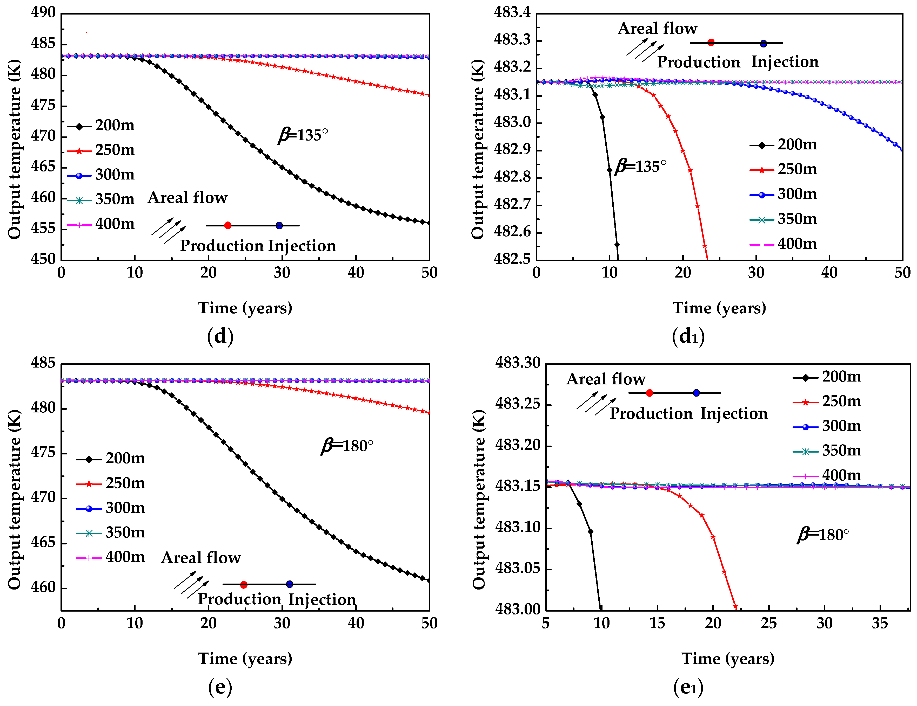
Figure 11.
Temperature variation of production wells with time at different flow rate (Where a1 is the partial details of the graphs a). (a) Evolution of output temperature during 50 years under different flow rate conditions under β = 0°; (a1) Local amplification of figure a. (b) Evolution of output temperature during 50 years under different flow rate conditions under β = 45°; (c) Evolution of output temperature during 50 years under different flow rate conditions under β = 90°; (d) Evolution of output temperature during 50 years under different flow rate conditions under β = 135°; (e) Evolution of output temperature during 50 years under different flow rate conditions under β = 180°.
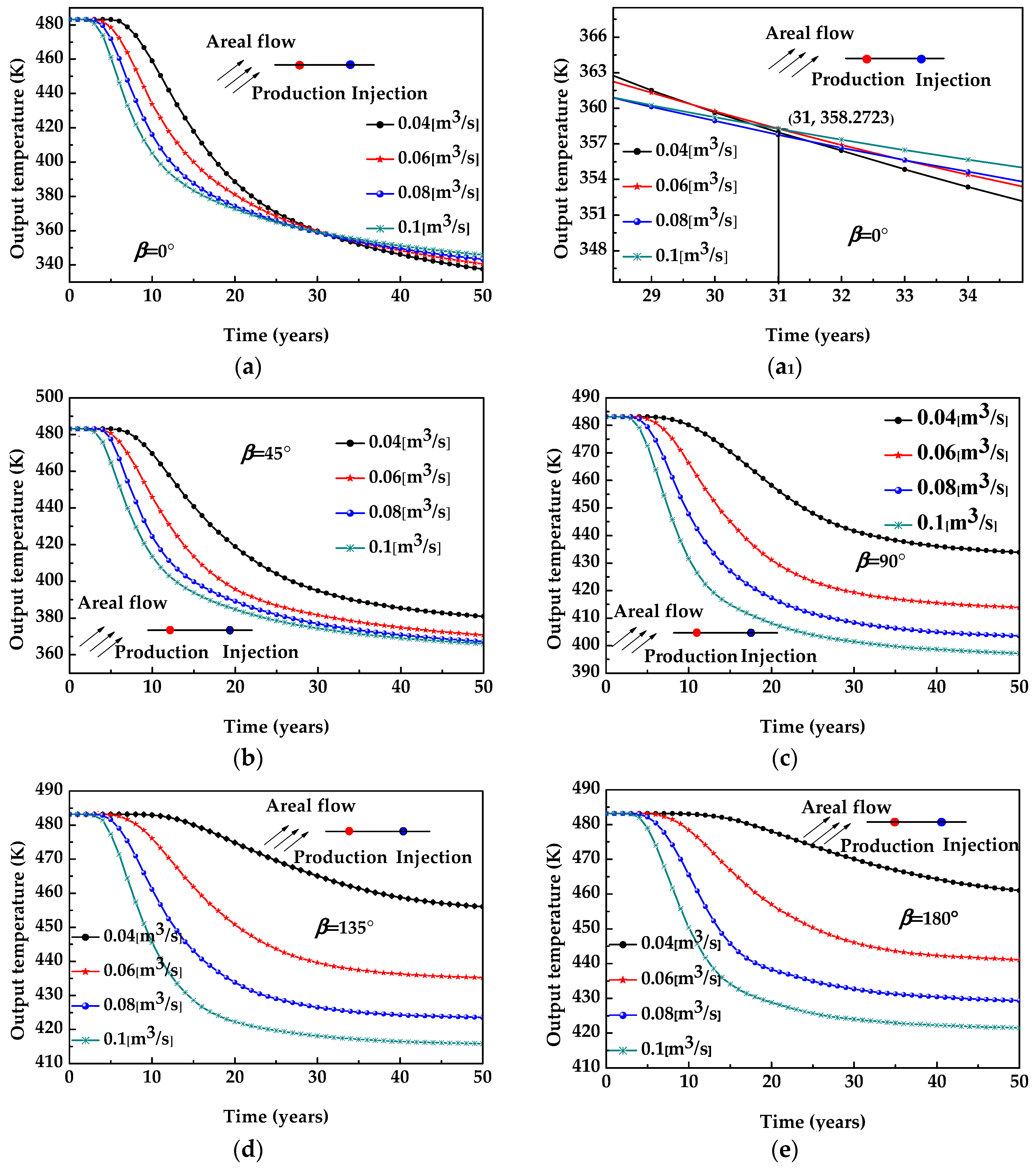
Figure 12.
Heat generation rate of EGS changes with time.

Figure 13.
Power generation of EGS with time.


Table 1.
Comparison of numerical simulation software for EGS exploitation.
| Simulation Software | Development Agency | Computational Method | Software Feature |
|---|---|---|---|
| COMSOL | COMSOL Co. Ltd. Stockholm, Sweden | FEM | Self-defining partial differential equation, automatic solution, automatic division of the grid, multiple physical problems can bearbitrarily coupled |
| FEHM | Operated by Los Alamos National Security, LLC for the U.S. Dept. of Energy’s NNSA | FEM | 3-dimensional complex geometries with unstructured grids saturated and unsaturated media simulation of production from gas hydrate reservoirs simulation of geothermal reservoirs non-isothermal, multi-phase flow of gas, water, oil non-isothermal, multi-phase flow of air, water non-isothermal, multi-phase flow of CO2, water and so on. |
| ECLIPSE | Schlumberger, Central and Eastern Europe: Hannover, Germany | FVM | For all types of reservoirs and degrees of complexity, structure, geology, fluids, and development schemes. ECLIPSE is a fully implicit, three-phase, 3D, general purpose black-oil simulator that includes several advanced and unique features. |
| Fluent | FLUENT Co. Ltd. Lebanon, NH, USA | FVM | Dynamic/deformed mesh technology mainlysolves the boundary motion, and the simulation fluid flow and heat transfer with high accuracy |
Table 2.
Main material parameters of single fracture model.
| Parameters | Symbols | Units | Values |
|---|---|---|---|
| Initial temperature of rock mass | Tr0 | °C | 180 |
| Temperature of fracture water | Tf0 | °C | 40 |
| Rock density | ρr | Kg/m3 | 2820 |
| Rock heat capacity | cr | J/kg·°C | 1170 |
| Rock heat conductivity | kr | W/m·°C | 2.80 |
| Density of fracture water | ρf | Kg/m3 | 1000 |
| Heat capacity of fracture water | cf | J/kg·°C | 4200 |
| Fracture flow velocity | uf | cm/s | 1 |
| Fracture aperture | δ | m | 0.01 |
| Fracture length | L | m | 100 |
Table 3.
Material parameters of enhanced geothermal system.
| Parameters | Symbols | Units | Values |
|---|---|---|---|
| Porous media permeability | к | m2 | 1.0 × 10⁻¹² |
| Porous media porosity | εp | 1 | 0.01 |
| Porous media density | ρp | kg/m3 | 2700 |
| Constant pressure heat capacity of porous media | cp.p | J/(kg·°C) | 1000 |
| Thermal conductivity of porous media | k | W/(m·°C) | 3 |
| Specific heat ratio of porous media | γp | 1 | 1 |
| Fracture porosity | εfr | 1 | 0.5 |
| Fracture permeability | кp | m2 | 1.0 × 10⁻¹⁰ |
| Fracture density | ρfr | kg/m3 | 1650 |
| Specific heat capacity of the fracture | cfr | J/(kg·°C) | 1000 |
| Thermal conductivity of fracture | kfr | W/(m·°C) | 4 |
| Fracture Width | dfr | m | 0.002 |
| Specific heat ratio of fracture | γfr | 1 | 1 |
| Constant pressure heat capacity of fluid | cp | J/(kg·°C) | 4200 |
| Thermal conductivity of fluid | kp | W/(m·°C) | 0 |
| Specific heat ratio of fluid | γ | 1 | 1 |
© 2018 by the authors. Licensee MDPI, Basel, Switzerland. This article is an open access article distributed under the terms and conditions of the Creative Commons Attribution (CC BY) license (http://creativecommons.org/licenses/by/4.0/).
Share and Cite
MDPI and ACS Style
Yao, C.; Shao, Y.; Yang, J. Numerical Investigation on the Influence of Areal Flow on EGS Thermal Exploitation Based on the 3-D T-H Single Fracture Model. Energies 2018, 11, 3026. https://doi.org/10.3390/en11113026
AMA Style
Yao C, Shao Y, Yang J. Numerical Investigation on the Influence of Areal Flow on EGS Thermal Exploitation Based on the 3-D T-H Single Fracture Model. Energies. 2018; 11(11):3026. https://doi.org/10.3390/en11113026
Chicago/Turabian StyleYao, Chi, Yulong Shao, and Jianhua Yang. 2018. "Numerical Investigation on the Influence of Areal Flow on EGS Thermal Exploitation Based on the 3-D T-H Single Fracture Model" Energies 11, no. 11: 3026. https://doi.org/10.3390/en11113026
Note that from the first issue of 2016, this journal uses article numbers instead of page numbers. See further details here.