Fuzzy Portfolio Optimization of Power Generation Assets

Abstract

Fuzzy theory is proposed as an alternative to the probabilistic approach for assessing portfolios of power plants, in order to capture the complex reality of decision-making processes. This paper presents different fuzzy portfolio selection models, where the rate of returns as well as the investor’s aspiration levels of portfolio return and risk are regarded as fuzzy variables. Furthermore, portfolio risk is defined as a downside risk, which is why a semi-mean-absolute deviation portfolio selection model is introduced. Finally, as an illustration, the models presented are applied to a selection of power generation mixes. The efficient portfolio results show that the fuzzy portfolio selection models with different definitions of membership functions as well as the semi-mean-absolute deviation model perform better than the standard mean-variance approach. Moreover, introducing membership functions for the description of investors’ aspiration levels for the expected return and risk shows how the knowledge of experts, and investors’ subjective opinions, can be better integrated in the decision-making process than with probabilistic approaches.

1. Introduction

The purpose of the portfolio selection problem is to find combinations of investment possibilities which best meet the objectives of the investor. This analysis needs various types of information and should be based on criteria which can provide some guidance about what is important and unimportant, or what is relevant and irrelevant. Although the weighting of these objectives and the criteria depend on the type of investor, the two that are common to all investors are expected return maximization and risk minimization. If investors are rational, they want the return to be high and prefer certainty to uncertainty. Moreover, the optimal portfolio enables the investor to mitigate risk and opportunities with respect to a wide range of alternatives.

The foundation of modern portfolio analysis was laid by Harry Markowitz in the middle of the 20th century [1]. He considered returns of assets as random variables and introduced the mean-variance approach. He identified the portfolio return as an expected return, which is a sum of the product between the asset’s expected return and its shares in the portfolio, and the risk measured as the volatility (variance) of the (stochastic) value of the expected return. Furthermore, he assumed the multivariate normal distribution for the rates of return and the quadratic form for the investor’s utility (preferences) function. The purpose of mean-variance portfolio (MVP) analysis is the maximization of the portfolio’s expected return and the minimization of the portfolios’s risk. Searching for efficient portfolios (“efficient” in this context means there exists no other portfolio with the same or a smaller variance that has a larger return, and no portfolio with the same or a larger return that has a smaller risk) could be conducted by solving one of two problems: (1) maximization of the portfolio’s expected return by a given accepted risk level or (2) minimization of the portfolio’s risk by some given required portfolio return level.

The methodology proposed by Markowitz has seen an extensive development since 1952 but also a lot of criticism. Trying to avoid some of the rigid assumptions of MVP analysis and to simplify the solution methodology, a number of alternative approaches have been proposed and applied. For example, the computational complexity connected with the mean-variance model (necessity of estimation of the variance and covariance matrix) led to the linearization of the objective function. Furthermore, the popularity among investors of other risk measures, such as mean absolute deviation (MAD), value at risk (VaR), expected shortfall (conditional value at risk—CVaR), or semi-variance, is growing.

The MAD model is one of the alternatives to the classic mean-variance model in which the measure of risk (variance) is replaced by the absolute deviation. Konno and Yamazaki [2] proposed the MAD model as a linear model for portfolio selection and tested its application on data from the Tokyo stock market. These authors observed that the MAD model can be used as an alternative to the Markowitz model because the calculated optimal portfolios and their performances are quite similar to each other. Moreover, a linear problem could be solved more easily than a quadratic one. Furthermore, the authors noticed that the MAD model could be used to tackle large-scale problems where a dense covariance matrix can occur, and that it does not require any specific type of return distribution. They also showed that the proposed method encompasses all properties of the MVP analysis. However, the method and its advantages were not widely appreciated in the financial engineering community and were criticized by statisticians. Konno and Koshizuka [3] reviewed some of the more important properties of the MAD portfolio optimization model. They pointed out that the MAD model is superior to the MVP model both theoretically and computationally, and that this model belongs to a class of mean-lower partial risk models, which are more adequate to problems with asymmetric return distributions. The MAD model proposed by Konno and Yamazaki [2] found interest among other researchers and applicaton to other financial markets. Application of the MAD model (based on the linear semi-mean-absolute deviation risk function) enabled Mansini and Speranza [4] to introduce new specifications derived from market structure and from operative constraints into the portfolio selection model of the Milan stock exchange. De Silva et al. [5] applied the MAD as well as the CVaR approach in order to avoid inefficient, low return, and/or high-risk portfolios on the Brazilian stock exchange. Furthermore, Liu [6] used the concept of the mean-absolute deviation function proposed by [2] when the asset returns from financial markets are represented by interval data. The author noticed that the ability to calculate the bounds of the investment return can help initiate wider applications in portfolio selection problems. A brief review of the variety of solvable linear programming portfolio optimization models presented in the literature, where several different risk measures (such as MAD or CVaR) were applied, can be found by Mansini et al. [7]. The authors discussed the relative and absolute form of these models and their applications.

The mean-variance portfolio selection model, and other existing portfolio selection models, are based on probability theory. However, as a number of empirical studies have shown, those probabilistic approaches only partly capture reality, in contrast to fuzzy sets theory. Fuzzy sets theory can be used for a better description of real systems (situations) that are very often uncertain and vague in different ways [8]. Zimmermann, in his seminal book [8], explains the vagueness, fuzziness, and uncertainty in real-world systems as well as the usefulness of the application of fuzzy sets theory in order to model uncertainty. He develops the formal framework of fuzzy mathematics and presents the survey of the most interesting applications of the theory.

Fuzzy sets theory and fuzzy logic, the latter of which is an extension of classic argumentation (conventional logic) to argumentation that is closer to humans, was introduced by Lotfi A. Zadeh [9]. In the classical set theory, objects can either belong to a set or not, and there are no intermediate steps of membership. In contrast, a fuzzy set also allows for blurred states. Zadeh ([9], p. 338) defines a fuzzy set as follows: “A fuzzy set is a class of objects with a continuum of grades of membership. Such a set is characterized by a membership (characteristic) function which assigns to each object a grade of membership ranging between zero and one”. The extension of fuzzy logic is possibility theory, introduced also by Zadeh [10] and advanced by Dubois and Prade [11]. Zadeh tries to explore some of the elementary properties of the possibility distribution concept and explains the importance of possibility theory, which arises from the fact that the information for the decisions is possibilistic rather than probabilistic in nature. Moreover, possibility theory is not a substitute for probability theory but deals with another kind of uncertainty. In possibility theory, the fuzzy variables are associated with possibility distributions in a similar way as random variables are with probability distributions. In contrast to probability theory, the possibility distribution function is defined by a so-called ‘membership function’ which describes the degree of affiliation of fuzzy variables. Membership functions which is a fundamental part of fuzzy sets theory, allows the gradual assessment of the membership of elements into the set and can characterize the fuzziness, have different forms. The most popular ones used are triangular, trapezoidal, or parabolic. However, other membership functions are hyperbolic, inverse-hyperbolic, exponential, logistic, or piecewise-linear.

Application areas for fuzzy sets theory are broad, ranging from different control systems, engineering, and consumer electronics to business economics, including decision theory [12], or financial problems, such as portfolio selection [13]. By using a fuzzy approach, the knowledge of experts, investors’ subjective opinions, but also quantitative and qualitative analysis, can be better integrated into decision problems. Wang and Zhu [14] and Fang et al. [13] give a survey of the progress made in recent years in the direction of fuzzy portfolio optimization. They present different portfolio selection models with fuzzy objectives and/or fuzzy constraints. One of the possibilities is that of using fuzzy numbers to define the coefficients of the objectives and constraints; another one is applying the so-called aspiration (or satisfaction) level. Another concept of fuzzy portfolio problems considers models with interval coefficients, where expected returns are treated as interval numbers, and where so-called pessimistic and optimistic satisfaction indices are introduced (for more information, see [15]). Furthermore, Tanaka and Guo [16] proposed the use of possibility distributions in order to model uncertainty in returns. They defined upper and lower possibility distributions which should reflect experts’ knowledge with regard to the portfolio selection problem.

The aim of this paper is to present a portfolio selection model for energy utilities by employing alternative risk measures, such as semi-mean-absolute deviation, which is one of the first attempts at the linearization of portfolio selection models, and comparing it with the standard mean-variance approach. Moreover, the contribution of this paper is an application of fuzzy sets theory to portfolio optimization problems in combination with alternative portfolio risk measures that can be more adequate for portfolios of real assets (such as power plants). The argument is that, in the case of power generation assets, the distribution of the power plant’s return measure and commodity prices as well as other parameters taken into consideration differ from the normal distribution assumed in the standard mean-variance portfolio approach, potentially causing biased results.

The remainder of this paper is organized as follows: Section 2 deals with the application of portfolio analysis to the energy sector and in particular to power generation mixes. In Section 3, fuzzy semi-mean-absolute deviation portfolio selection models and a “return” definition for power generation mixes are introduced. Section 4 shows an empirical example for the presented methodologies. Section 5 provides some conclusions.

2. Applications of Portfolio Analysis to Power Generation Assets

The energy utilities are confronted with a very diverse range of resource options in their energy planning, but also a dynamic, complex, and uncertain future. Financial investors are used to dealing with uncertainty and commonly evaluate such problems with portfolio theory. According to portfolio theory, they could choose a specific risk level and then aim to maximize the portfolio’s return. Furthermore, the diversification of portfolio assets is the best means of hedging future risk. Therefore, mean-variance portfolio theorists have found a new application field in the energy sector, and the theory seems to be a well-suited complementary methodology to the problem of planning and evaluating power portfolios and strategies.

The first application of portfolio theory to the energy sector was presented by Bar-Lev and Katz [17]. They applied the Markowitz portfolio approach to optimize the fossil fuel mix for electric utilities in the US market and examined whether the power utilities are efficient users of fossil fuels. More specifically, they considered a two-dimensional optimization problem with fuel cost and risk minimization. More recent literature contains further applications of portfolio theory to energy markets in different countries or regions from a utility point of view (for a recent review, see [18]). For example, Awerbuch and Berger [19] used MVP analysis for the electricity market in the European Union. They proposed a more complex model where fuel costs and also operating and capital costs were explicitly considered. Their results indicate that the current EU electricity mix is sub-optimal from a risk-return perspective. Furthermore, they conclude that fixed-cost technologies, such as many of those based on renewables, must be a part of any efficient portfolio. Roques et al. [20] considered the portfolio problem based on the MVP methodology from a cost perspective, but also added revenues and included the net present value (NPV) of the investment. They analyzed energy markets in the UK, and concluded that the optimal portfolio consists of natural-gas-combined cycle (NGCC) and a few nuclear power plants. Further applications of portfolio theory to the energy sector can be found in [18,21]. In [21], the cost approach was again applied and electricity production costs considered, which included fuel costs together with operating, capital, and external costs. Moreover, for this study of the Swiss and the U.S. energy market, the authors adopted seemingly unrelated regression estimation (SURE). The Swiss power generation mix was also the goal of the analysis presented in [22]. They are the first to implement the NPV criterion for portfolio analysis, following the Markowitz model. Moreover, they explicitly differentiated between base-load and peak-load technologies. In the work of Borchert and Schemm [23], the application of the CVaR as a risk measure in portfolio analysis for wind power projects in Germany was presented. Glensk et al. [24] also applied CVaR as a risk measure, but instead of power generation assets they analyzed portfolios of contracts from the European Energy Exchange (EEX) and the Polish Power Exchange (POLPX). They further pointed out that the proposed approach can be useful, especially for retailers on both markets, but that the impact of negative energy prices, as found e.g., on the EEX, should also be investigated.

The studies mentioned above reflect a considerable and growing interest in applying portfolio analysis on (liberalized) energy markets. Moreover, they point out different definitions of return and risk used by authors applying MVP theory to power generation portfolios. Analogically to the financial markets, the decision-making process in energy planning is complex and multidimensional. Economic, social, and environmental aspects; technical parameters; and different risks have to be taken into account. Regarding all these different aspects, the risk connected to electricity price, fuel cost, carbon dioxide cost, operation and maintenance costs, capital cost, but also to the capacity factor of a power plant, affect the measure of return and thus also the decision-making process and outcome. Application of portfolio theory can help to eliminate these risks and to explain the complex interactions between these parameters.

When applying portfolio theory to power generation mixes, appropriate definitions of return and risk are needed. Project evaluation methods and measures (such as net present value, internal and modified internal rate of return, profitability index, payback or discounted payback time) commonly used in finance management could also be useful proxies for the construction of power generation mixes. Each of these measures give different pieces of relevant and valuable information needed in the decision-making process. However, the net present value and the internal rate of return are the most often ones used. According to the short literature review presented, the NPV criterion is already one useful profitability indicator for energy projects and power generation selection problems, next to the annual expected return.

3. Model Specification

In this section, we present the model formulation for the selection of the optimal power generation mix, considering the semi-mean-absolute deviation as a risk measure and assuming that each rate of return is a possibilistic variable.

3.1. Semi-Mean-Absolute Deviation (SMAD) Model

In general, the portfolio optimization problem is a two-dimensional optimization model, where portfolio risk is minimized and return is maximized. Most dissatisfaction with the variance introduced by Markowitz as a risk measure stems from the fact that it does not differentiate between gains and losses. Moreover, Harry Markowitz himself and William Sharpe, among other economists, acknowledge that the original modern portfolio theory formulation has important limitations ([25], p. 428): “Under certain conditions, the mean-variance approach can be shown to lead to unsatisfactory predictions of behavior. Markowitz suggests that a model based on the semi-variance would be preferable; in light of the formidable computational problems; however, he bases his analysis on the variance and standard deviation.” As shown in [26], the mean-absolute deviation as a measure of variability is less sensitive to outliers, and equivalent to mean-variance under the assumption of the normal distribution of the returns. Furthermore, the author shows that the MAD model possesses several advantageous theoretical properties, such that all capital asset pricing model relations for the mean-variance model also hold for the MAD model. Moreover, the MAD model is more compatible with the fundamental principle of rational decision-making. Despite the fact that the mean-variance Markowitz (1952) model is a solid, well-known method, which laid the foundation for portfolio theory, it has been proven that MAD produces similar portfolio returns [5,27], which makes us confident in MAD’s optimization ability. Considering this alternative definition of risk MAD, as proposed by Konno and Yamazaki [2], the portfolio rate of return, $R_p$, is given as:

$$R_p=E\left[\sum _{i=1}^n{R}_i{x}_i\right]=\sum _{i=1}^{n}E\left(R_i\right)x_i,$$

(1)

and defined as the expected value of a sum of the product between the assets’ expected return, $R_i$, and its shares in the portfolio, $x_i$, and the portfolio risk, $w_p$, defined by the expected value of the mean absolute deviation between the realization of the portfolio’s rate of return and its expected value, as:

$$w_p=E\left[\left|\sum _{i=1}^n{R}_i{x}_i-E\left[\sum _{i=1}^n{R}_i{x}_i\right]\right|\right].$$

(2)

Regarding these definitions of portfolio return and risk, a two-dimensional optimization problem can be formulated as follows:

$$E\left[\left|\sum _{i=1}^n{R}_i{x}_i-E\left[\sum _{i=1}^n{R}_i{x}_i\right]\right|\right]\to min,$$

$$\begin{array}{c}{\displaystyle \sum _{i=1}^n}E\left(R_i\right)x_i\to max,\end{array}$$

(3)

$$\sum _{i=1}^n{x}_i=1,$$

$$0\le x_i\le x_{i,max},$$

where $x_{i,max}$ is the maximal share of asset i in the portfolio.

Assuming that the measure of risk is defined through the mean absolute deviation of the portfolio’s rate of return below the average (for the investor, only the downside risk is problematic, and thus actually relevant) the semi-mean-absolute deviation portfolio selection model can be specified as:

$$E\left[\left|min\left\{0,\sum _{i=1}^n{R}_i{x}_i-E\left[\sum _{i=1}^n{R}_i{x}_i\right]\right\}\right|\right]\to min,$$

$$\begin{array}{c}{\displaystyle \sum _{i=1}^n}E\left(R_i\right)x_i\to max,\end{array}$$

(4)

$$\sum _{i=1}^n{x}_i=1,$$

$$0\le x_i\le x_{i,max}.$$

The semi-mean-absolute deviation belongs to the favorite risk measure used in portfolio selection models. In contrast to the variance, the semivariance as well as the CVaR (mentioned in Section 1) fulfill all desirable properties of a “good” risk measure, and the SMAD satisfies two out of four properties of coherent risk measures (see [28]), such as positive homogenity and subadditivity [29,30]. Nevertheless, the standard deviation, mean absolute deviation as well as mean absolute lower and upper semi-deviation belong to the general deviation risk measures introduced by Rockafellar et al. [31,32] as an extension of standard deviation, but they need not to be symmetric with respect to the upside and downside value of the random variable. The authors developed a theory of deviation measures axiomatically, presenting key examples and tracing the relationships with concepts of coherent risk measures. The main possible advantage of mean absolute deviation and its downside version is the relation to linear programming computations of optimal portfolios. Moreover, as shown in [33,34], because the MAD is a symmetric measure and the absolute semi-deviation is its half.

Regarding the considerations presented by Konno and Koshizuka [3] and Speranza [35], the equivalent to the semi-mean-absolute deviation model in (4) is given as:

$$\frac{1}{T}\sum _{t=1}^T{d}_t\to min,$$

$$\sum _{i=1}^{n}E\left(R_i\right)x_i\to max,$$

$$\begin{array}{c}{d}_t\ge -{\displaystyle \sum _{i=1}^n}\left(R_{it}-E\left(R_i\right)\right)x_i,\end{array}$$

(5)

$$d_t\ge 0,$$

$$\sum _{i=1}^n{x}_i=1,$$

$$0\le x_i\le x_{i,max}.$$

3.2. Fuzzy Semi-Mean-Absolute Deviation (FSMAD) Model

The imperfect knowledge about returns and the resulting uncertain environment imply that the use of precise mathematics to model a complex system is insufficient. In order to capture the complex reality of decision-making problems, fuzzy sets theory is proposed as an alternative to the commonly used probabilistic approach. Different studies about fuzzy portfolio selection show that different elements can be fuzzified. Some of them suggest the use of a possibility distribution to capture model uncertainty on returns, while others propose fuzzy formulations. In this paper, we present only some of them, with a specific focus on the application to the energy sector.

Assuming that each rate of return, $R_i$, is a possibilistic variable, the simple conversion of model (5) presented above is replacing the expected value of the rate of return for asset i, $E\left(R_i\right)$, by an adequate fuzzy mean value. This fuzzy mean value depends on the form of membership function assumed. Considering $R_i$ as a triangular fuzzy variable determined by triplet (a, $\alpha$, $\beta$) of crisp numbers with center a, left-width $\alpha >0$ and right-width $\beta >0$, the interval-valued possibilistic mean, $M_{tr}\left(R_i\right)$, proposed by Carlsson and Fullér [36], is given as:

$$M_{tr}\left(R_i\right)=a+\frac{\beta -\alpha }{6}.$$

(6)

Triangular membership functions are mostly used for fuzzy logic control problems. The motivation behind their utilization stems from its simplicity. However, for many other applications, such as decision-making problems, triangular membership functions are not appropriate, and using a trapezoidal membership function is more reasonable. For a trapezoidal membership function [36], the interval-valued possibilistic mean value, $M_{trap}\left(R_i\right)$, with a tolerance interval [a, b] and left- and right-width $\alpha$ and $\beta$, respectively, is given by

$$M_{trap}\left(R_i\right)=\frac{a+b}{2}+\frac{\beta -\alpha }{6}.$$

(7)

Some applications of this approach on the financial markets are proposed and shown by [13,37,38,39,40], among others. These authors considered portfolio selection models with both the variance as a risk measure as well as the mean-absolute deviation.

Taking into consideration a trapezoidal membership function and its interval-valued possibilistic mean value, the SMAD portfolio selection model (5) has to be reformulated. Moreover, regarding one of the optimization approaches mentioned in Section 1, the risk minimization problem for a given desired portfolio return level, $R_0$, will be considered, and is specified as:

$$\frac{1}{T}\sum _{t=1}^T{d}_t\to min,$$

$$\sum _{i=1}^n{M}_{trap}\left(R_i\right)x_i\ge R_0,$$

$$\begin{array}{c}{d}_t+{\displaystyle \sum _{i=1}^n}\left(R_{it}-M_{trap}\left(R_i\right)\right)x_i\ge 0,\end{array}$$

(8)

$$d_t\ge 0,$$

$$\sum _{i=1}^n{x}_i=1,$$

$$0\le x_i\le x_{i,max}.$$

Let us further propose that the return $R_i$ is a fuzzy variable determined by a trapezoidal membership function with a tolerance interval [$a_i$, $b_i$] and left- and right-width ${\alpha }_i$ and ${\beta }_i$, respectively ($R_i=(a_i,b_i,{\alpha }_i,{\beta }_i)$). Vercher et al. [38] assumed that the left and the right reference functions are all of the same shape and are presented as the linear combination, which expresses the total fuzzy return on a portfolio, as in:

$$\begin{array}{c}{R}_p={\displaystyle \sum _{i=1}^n}{R}_i{x}_i=\left({\displaystyle \sum _{i=1}^n}{a}_i{x}_i,{\displaystyle \sum _{i=1}^n}{b}_i{x}_i,{\displaystyle \sum _{i=1}^n}{\alpha }_i{x}_i,{\displaystyle \sum _{i=1}^n}{\beta }_i{x}_i\right)=\\ =\left(R_{pa}\left(x\right),R_{pb}\left(x\right),R_{p\alpha }\left(x\right),R_{p\beta }\left(x\right)\right).\end{array}$$

(9)

Regarding the semi-mean-absolute deviation portfolio selection model (4), the above-presented fuzzy portfolio return (9), and following deliberations presented by [38], the portfolio selection model is defined as an optimization problem, which, for a given required return level, $R_0$, yields a minimum-risk portfolio and which can be formulated as:

$$\sum _{i=1}^n\left(b_i-a_i+\frac{1}{3}\left({\alpha }_i+{\beta }_i\right)\right)x_i\to min,$$

$$\begin{array}{c}{\displaystyle \sum _{i=1}^n}\left(\frac{1}{2}\left(a_i+b_i\right)+\frac{1}{6}\left({\beta }_i-{\alpha }_i\right)\right)x_i\ge R_0,\end{array}$$

(10)

$$\sum _{i=1}^n{x}_i=1,$$

$$0\le x_i\le x_{i,max}.$$

As mentioned before, investment decisions are generally influenced by uncertain or hardly predictable social and economic circumstances. In such cases, the application of optimization methods is not always the best in comparison to the satisfaction approach. Especially in portfolio selection problems, the investor always has certain objective values concerning the expected return and a certain degree of risk. In problems encountered in a real world, some vague aspiration level is based on experiences and knowledge of decision-makers. Therefore, it is more natural to denote an individual’s aspiration level as a fuzzy number. Additionally, the concept of employing fuzzy numbers to express an investor’s aspiration level is also connected with choosing an adequate membership function for model formulation. Watada [15] was the first to propose the use of a trapezoidal membership function in order to describe the return and risk aspiration level. Based on the Bellman–Zadeh maximization principle [12], he introduced a two-dimensional Markowitz portfolio selection problem with a certain aspiration level as fuzzy numbers. However, he then also discovered that by employing this function, there exist some difficulties when solving the portfolio selection problem. In order to avoid these problems, Watada proposed a nonlinear logistic membership function, arguing that a logistic function is more appropriate to vague goal levels of investors and, in addition, that the trapezoidal function (considered at first) is an approximation of the logistic function.

Taking into account the proposition and assumptions introduced by Watada [15], the logistic membership function for the portfolio’s expected return and risk are given by ${\mu }_R\left(R_p\right)$ and ${\mu }_w\left(w_p\right)$, respectively, as:

$${\mu }_R\left(R_p\right)=\frac{1}{1+exp(-{\alpha }_R(R_p-R_M))},$$

(11)

$${\mu }_w\left(w_p\right)=\frac{1}{1+exp\left({\alpha }_w(w_p-w_M)\right)},$$

(12)

where $R_M$ and $w_M$ are the mid-points (of the expected return and risk, respectively) at the membership function value $\lambda$ = 0.5, and ${\alpha }_R$ and ${\alpha }_w$ determine the shape of the membership functions ${\mu }_R\left(R_p\right)$ and ${\mu }_w\left(w_p\right)$, respectively. The two parameters $R_M$ and $w_M$ are determined by $\frac{R_s+R_n}{2}$ and $\frac{w_s+w_n}{2}$ where $R_s$ is sufficiency and $R_n$ the necessity level for the return, and $w_s$ is sufficiency and $w_n$ the necessity level for the risk measure. The values of the sufficiency and necessity levels for return and risk can be provided by the decision-maker, although the well-known (and in this work employed) method is the one proposed by Zimmermann [41].

Considering the Bellman–Zadeh maximization principle [12], the general portfolio selection problem with aspiration levels can be formulated as follows:

$$\lambda \to max,$$

$${\mu }_R\left(R_p\right)\ge \lambda ,$$

$${\mu }_w\left(w_p\right)\ge \lambda ,$$

$$\begin{array}{c}{\displaystyle \sum _{i=1}^n}{x}_i=1,\end{array}$$

(13)

$$0\le x_i\le x_{i,max},$$

$$\lambda \ge 0.$$

Reconsidering the semi-mean-absolute deviation portfolio selection model (5) and by replacing ${\mu }_R\left(R_p\right)$ and ${\mu }_w\left(w_p\right)$ in model (13) with Equations (11) and (12), respectively, the following problem results:

$$\lambda \to max,$$

$$\lambda +exp\left(-{\alpha }_R\left(\sum _{i=1}^{n}E\left(R_i\right)x_i-R_M\right)\right)\lambda \le 1,$$

$$\lambda +exp\left({\alpha }_w\left(\frac{1}{T}\sum _{t=1}^T{d}_t-w_M\right)\right)\lambda \le 1,$$

$$\begin{array}{c}{d}_t+{\displaystyle \sum _{i=1}^n}(R_{it}-E\left(R_i\right))x_i\ge 0,\end{array}$$

(14)

$$d_t\ge 0,$$

$$\sum _{i=1}^n{x}_i=1,$$

$$0\le x_i\le x_{i,max},$$

$$\lambda \ge 0.$$

The two exponential constraints in the above-presented model can be transformed into

$${\alpha }_R\left(\sum _{i=1}^{n}E\left(R_i\right)x_i-R_M\right)\ge log\frac{\lambda }{1-\lambda },$$

(15)

$$-{\alpha }_w\left(\frac{1}{T}\sum _{t=1}^T{d}_t-w_M\right)\ge log\frac{\lambda }{1-\lambda }.$$

(16)

Replacing $\Lambda =log\frac{\lambda }{1-\lambda }$ in (15) and (16), the model formulation (14) is equivalent to:

$$\Lambda \to max,$$

$${\alpha }_R\sum _{i=1}^{n}E\left(R_i\right)x_i-\Lambda \ge {\alpha }_R{R}_M,$$

$${\alpha }_w\frac{1}{T}\sum _{t=1}^T{d}_t+\Lambda \le {\alpha }_w{w}_M,$$

$$\begin{array}{c}{d}_t+{\displaystyle \sum _{i=1}^n}(R_{it}-E\left(R_i\right))x_i\ge 0,\end{array}$$

(17)

$$d_t\ge 0,$$

$$\sum _{i=1}^n{x}_i=1,$$

$$0\le x_i\le x_{i,max},$$

$$\Lambda \ge 0.$$

According to the parameters ${\alpha }_R$ and ${\alpha }_w$, which determine the shape of the membership functions, the aspiration levels can be described accurately. The calculation of the parameters $\alpha$ depends on the membership function used in the model. For the membership function presented in this work for the return (11) and risk (12), ${\alpha }_R=\frac{6.91}{0.5(R_s-R_n)}$ and ${\alpha }_w=\frac{6.91}{0.5(w_s-w_n)}$, respectively (for more information, see [42]). Therefore, the portfolio selection model presented is convenient for different investors and their individual investment strategies. The application of this model for onshore wind power plants can be found in [43].

3.3. Return Definition for the Power Generation Portfolio Selection Problem

As mentioned in Section 2 above, many of the differences in the applications of portfolio analysis to energy markets are connected with the choice of the selection criteria used (and particularly differing return and risk definitions). Power generation mix problems have their specific character connected with the evaluation of power plants. In an evaluation process, different measures and methods borrowed from finance can be used. The choice about which of them to adopt depends on the decision-maker and her/his expectations regarding portfolio analysis. By searching for an appropriate and useful proxy, not only costs and revenues should be taken into consideration, but also technical parameters and the expected (remaining) lifetimes of the power plants concerned. Furthermore, an important point in the analysis is the impact of new investments on the existing portfolio. The massive changes in worldwide energy industries are the results of a number of factors, such as the increase in energy demand, growing industrialization processes, environmental policy and resource limitations. Many countries and energy providers are obliged to reconstruct (renew, expand, etc.) their power generation mix and to develop new, more sustainable possibilities of producing energy (especially carbon-free or low-carbon technologies).

Regarding all these aspects, the NPV approach appears to be not a perfect one but a relatively suitable measure as a portfolio selection criterion (see, e.g., [20] or [22] where the NPV was applied for the selection of power generation assets) both for new investments and also for existing power plants. Another possibility is the use of the annual return as a selection criterion. In contrast to the NPV, the annual return is a static measure and requires that the forecasts of all factors are taken into consideration in the analysis (see, e.g., [44]). Following an approach similar to the one used in [20,22], the objective variable is defined as the NPV of the investments. A favorable characteristic of the NPV approach is the allowance of a risk- and time-adjusted discounting, thus respecting the time value of different investments. Especially in the power supply industry, where investment horizons often span several decades, this is a very important point. It is based upon the discounted cash-flow technique and given by:

$$NPV=\sum _{t=0}^T\frac{C{F}_t}{{(1+WACC)}^t},$$

(18)

where $C{F}_t$ denotes the annual cash flow and the WACC (weighted average cost of capital) is used as the discount rate.

The estimation of cash flows for power plants during the operation time requires input data, such as revenues obtained from energy production, fuel costs, carbon dioxide mitigation costs, operation and maintenance costs, capital costs as well as the depreciation rate. The calculation of a cash flow starts with the determination of earnings before interest and taxes (EBIT), which is given as the difference between revenues and costs including depreciation. After tax subtraction, earnings before interest and after tax (EBIAT) are obtained. Finally, to achieve the cash flow, depreciation expenses are added to EBIAT (for more information, see e.g., [45]).

4. Results

This section presents several empirical applications of the above-described models for energy generation mixes. Considering power plants (in this case, existing power plants owned by E.ON in various location Germany and new investments announced by E.ON), we use the project’s NPV (in €/kW) as a proxy for portfolio selection, and risk is defined as the semi-mean-absolute deviation from the expected return (also in €/kW). All necessary information about the power plants considered, as well as their economic and technical data needed for the NPV estimation undertaken by Monte Carlo Simulation (MCS) and using the ORACLE^® Crystal Ball software (version 11.1), are reported in detail in [44,46], respectively.

The calculations of efficient portfolios were made for three different fuzzy set models: FSMAD Model 1 (= model (8)), FSMAD Model 2 (= model (10)), and FSMAD Model 3 (= model (17)). As an extension, a comparison of the presented results of these three models with the classic MV (mean-variance) model and with the SMAD (semi-mean-absolute deviation) model is also provided. The classic MV model was proposed by [1]; it is a portfolio selection model with the standard deviation used as a risk measure. This is a two-objective optimization problem, specified as:

$$\begin{array}{c}\hfill \begin{array}{c}{\displaystyle \sum _{i=1}^n}{x}_i^2{\sigma }_i^2+2{\displaystyle \sum _{i=1}^{n-1}}{\displaystyle \sum _{j=i+1}^n}{x}_i{x}_j{\sigma }_i{\sigma }_j{\rho }_{ij}\to min,\\ {\displaystyle \sum _{i=1}^n}E\left(R_i\right)x_i\to max,\\ {\displaystyle \sum _{i=1}^n}{x}_i=1\mathrm{and}0\le x_i\le x_{i,max},\end{array}\end{array}$$

where ${\sigma }_i^2$ denotes the variance of component asset i, ${\sigma }_i$ the volatility of asset i, and ${\rho }_{ij}$ the correlation coefficient between i and j. Efficient frontiers were obtained through the implementation of linear and quadratic programming in the dynamic, object-oriented programming language Python 2.6.

4.1. FSMAD Model for Power Generation Portfolios

Figure 1a–c show the efficient frontiers for existing power plants and all announced new investments obtained by using the FSMAD models presented in Section 3. Figure 1a shows the efficient frontiers where the projects’ return is considered as a possibilistic variable with the trapezoidal membership function and adequate fuzzy mean value. We observe that the increase of the return (NPV/installed capacity) is faster than the risk increase. Comparing Figure 1a with Figure 1b, where efficient frontiers are obtained by application of FSMAD Model 2, the shifting of the efficient frontiers can be noticed. The efficient portfolios depicted in Figure 1b for some specific return level have higher risk levels than the efficient portfolio presented in Figure 1a, which were obtained with another fuzzy approach to portfolio selection. Considering the investor’s aspiration levels, FSMAD Model 3 was analyzed as well and the results are shown in Figure 1c. In this case, the set of efficient portfolios is significantly smaller than for the two models presented first. Furthermore, by comparing Figure 1a and Figure 1c, one can observe that the efficient portfolios obtained by using FSMAD Model 3 (Figure 1c) from the upper part of the efficient frontiers depicted in Figure 1a (FSMAD Model 1). From inspection of Figure 1d, this outcome becomes even more clear.

Table A1. Efficient portfolios according to FSMAD Model 1 for existing technologies.

	Efficient Portfolios
Technologies	P1	P2	P3	P4	P5	P6
Biomass	0.07%	0.07%	0.07%	0.07%	0.07%	0.07%
CCGT	9.19%	7.13%	0.00%	0.00%	8.47%	9.19%
CHP	8.53%	8.53%	8.53%	8.53%	8.53%	5.70%
GT gas	3.24%	3.24%	3.24%	3.24%	0.00%	0.00%
GT oil	7.24%	7.24%	7.24%	7.24%	6.50%	0.00%
Hard coal	45.67%	45.67%	44.19%	11.01%	0.00%	8.61%
Hydro	14.95%	14.95%	14.95%	14.95%	14.95%	14.95%
Lignite	8.22%	0.00%	0.00%	1.69%	8.22%	8.22%
Nuclear	2.46%	12.74%	21.35%	52.84%	52.84%	52.84%
Onshore	0.42%	0.42%	0.42%	0.42%	0.42%	0.42%
NPV [€/kW]	632.71	750.00	900.00	1550.00	1650.00	1700.00
Risk [€/kW]	215.26	232.02	258.79	386.84	414.56	432.02

,

Table A2. Efficient portfolios according to FSMAD Model 1 for existing technologies combined with new investments.

	Efficient Portfolios
Technologies	P1	P2	P3	P4	P5	P6	P7	P8	P9
Biomass	0.06%	0.06%	0.06%	0.06%	0.06%	0.06%	0.06%	0.06%	0.06%
CCGT	16.36%	16.36%	16.36%	15.33%	5.93%	0.00%	0.00%	7.83%	7.83%
CHP	7.26%	7.26%	7.26%	7.26%	7.26%	7.26%	7.26%	7.26%	0.55%
GT gas	2.76%	2.76%	2.76%	2.76%	2.76%	2.76%	2.76%	2.76%	0.00%
GT oil	6.17%	6.17%	6.17%	6.17%	6.17%	6.17%	6.17%	6.17%	0.00%
Hard coal	48.76%	43.48%	38.88%	38.88%	38.88%	38.88%	21.73%	9.53%	22.74%
Hydro	12.73%	12.73%	12.73%	12.73%	12.73%	12.73%	12.73%	12.73%	12.73%
Lignite	1.79%	7.00%	2.70%	0.00%	0.00%	0.00%	0.92%	7.00%	7.00%
Nuclear	0.00%	0.07%	8.97%	12.69%	22.10%	28.03%	44.98%	44.98%	44.98%
Offshore	3.76%	3.76%	3.76%	3.76%	3.76%	3.76%	3.76%	3.76%	3.76%
Onshore	0.36%	0.36%	0.36%	0.36%	0.36%	0.36%	0.36%	0.36%	0.36%
NPV [€/kW]	479.71	550.00	700.00	750.00	950.00	1050.00	1400.00	1500.00	1550.00
Risk [€/kW]	208.47	214.14	230.58	237.33	266.57	284.00	352.95	380.93	400.58

,

Table A3. Efficient portfolios according to FSMAD Model 2 for existing technologies.

	Efficient Portfolios
Technologies	P1	P2	P3	P4	P5
Biomass	0.07%	0.07%	0.07%	0.07%	0.07%
CCGT	9.19%	4.17%	0.00%	0.00%	9.19%
CHP	8.53%	8.53%	8.53%	8.53%	5.70%
GT gas	3.24%	3.24%	3.24%	0.00%	0.00%
GT oil	7.24%	7.24%	7.24%	0.00%	0.00%
Hard coal	45.67%	45.67%	44.19%	9.56%	8.61%
Hydro	14.95%	14.95%	14.95%	14.95%	14.95%
Lignite	8.22%	0.00%	0.00%	6.38%	8.22%
Nuclear	2.46%	15.71%	21.35%	52.84%	52.84%
Onshore	0.42%	0.42%	0.42%	0.42%	0.42%
NPV [€/kW]	632.71	800.00	900.00	1600.00	1700.00
Risk [€/kW]	450.35	494.73	529.21	814.72	882.27

,

Table A4. Efficient portfolios according to FSMAD Model 2 for existing technologies combined with new investments.

	Efficient Portfolios
Technologies	P1	P2	P3	P4	P5	P6	P7	P8
Biomass	0.06%	0.06%	0.06%	0.06%	0.06%	0.06%	0.06%	0.06%
CCGT	16.36%	16.36%	16.36%	13.10%	2.96%	0.00%	0.00%	7.26%
CHP	7.26%	7.26%	7.26%	7.26%	7.26%	7.26%	7.26%	7.26%
GT gas	2.76%	2.76%	2.76%	2.76%	2.76%	2.76%	0.00%	0.00%
GT oil	6.17%	6.17%	6.17%	6.17%	6.17%	6.17%	6.17%	0.00%
Hard coal	48.76%	41.33%	38.88%	38.88%	38.88%	36.39%	24.00%	23.23%
Hydro	12.73%	12.73%	12.73%	12.73%	12.73%	12.73%	12.73%	12.73%
Lignite	1.79%	7.00%	2.70%	0.00%	0.00%	0.00%	0.68%	7.00%
Nuclear	0.00%	2.23%	8.97%	14.93%	25.07%	30.52%	44.98%	44.98%
Offshore	3.76%	3.76%	3.76%	3.76%	3.76%	3.76%	3.76%	3.76%
Onshore	0.36%	0.36%	0.36%	0.36%	0.36%	0.36%	0.36%	0.36%
NPV [€/kW]	479.71	600.00	700.00	800.00	1000.00	1100.00	1400.00	1500.00
Risk [€/kW]	432.38	456.76	477.07	502.51	561.46	597.25	715.97	775.99

,

Table A5. Efficient portfolios according to FSMAD Model 3 for existing technologies.

	Efficient Portfolios
Technologies	P1	P2	P3	P4
Biomass	0.07%	0.07%	0.07%	0.07%
CCGT	0.00%	0.00%	0.54%	9.19%
CHP	8.53%	8.53%	8.53%	0.05%
GT gas	3.24%	0.00%	0.00%	0.00%
GT oil	7.24%	7.01%	0.00%	0.00%
Hard coal	10.65%	7.95%	14.43%	14.25%
Hydro	14.95%	14.95%	14.95%	14.95%
Lignite	2.05%	8.22%	8.22%	8.22%
Nuclear	52.84%	52.84%	52.84%	52.84%
Onshore	0.42%	0.42%	0.42%	0.42%
NPV [€/kW]	1567.28	1635.69	1676.93	1739.59
Risk [€/kW]	394.61	413.28	426.46	450.84

and

Table A6. Efficient portfolios according to FSMAD Model 3 for existing technologies combined with new investments.

	Efficient Portfolios
Technologies	P1	P2	P3	P4	P5
Biomass	0.06%	0.06%	0.06%	0.06%	0.06%
CCGT	0.00%	0.00%	0.00%	2.15%	7.83%
CHP	7.26%	7.26%	7.26%	7.26%	0.00%
GT gas	2.76%	2.76%	0.00%	0.00%	0.00%
GT oil	6.17%	6.17%	5.04%	0.00%	0.00%
Hard coal	23.07%	21.26%	18.81%	21.70%	23.29%
Hydro	12.73%	12.73%	12.73%	12.73%	12.73%
Lignite	0.00%	0.66%	7.00%	7.00%	7.00%
Nuclear	43.84%	44.98%	44.98%	44.98%	44.98%
Offshore	3.76%	3.76%	3.76%	3.76%	3.76%
Onshore	0.36%	0.36%	0.36%	0.36%	0.36%
NPV [€/kW]	1378.85	1408.78	1483.60	1519.44	1566.99
Risk [€/kW]	351.58	357.96	378.59	390.05	411.68

in the Appendix show the exact compositions of the efficient portfolios presented in Figure 1a,c. The models analyzed in this work contain restrictions regarding the maximal share of each technology allowed in the power generation mix. Such restrictions are necessary from a technical point of view and ensure that all resulting portfolios are technically feasible.

Additional information obtained from this analysis is related to new investments taken under consideration. Especially in Figure 1a,b, in some cases, efficient frontiers for existing technologies and new investments are located above the efficient frontiers obtained for the existing technologies only. It means that including these investments in the existing power generation mix can apparently improve the efficiency of the portfolio.

4.2. Comparative Analysis

The second part of our analysis shows the comparison of results obtained between the fuzzy portfolio selection models with the well-known mean-variance portfolio selection model proposed by Markowitz, and with the SMAD model, the latter of which is used as a benchmark model for our study as well.

Figure 2 presents the location of the efficient frontiers obtained for FSMAD Model 1 and the SMAD Model. The first conclusion is that both models give more or less the same results. The very similar shape and position of the curves can be explained by the very similar arithmetic and fuzzy mean values obtained by Monte Carlo simulation. Nevertheless, closer inspection shows that the efficient frontier printed in blue (FSMAD Model 1) is located slightly above the efficient frontier printed in red (SMAD Model) and in green (FSMAD Model 1 regarding new investments); it is also located slightly above the frontier printed in black (SMAD Model with consideration of new investments). Furthermore, a more rigorous analysis of the expected NPV and risk levels for the efficient portfolios presented in Table A1 and

Table A9. Efficient portfolios according to the SMAD Model for existing technologies.

	Efficient Portfolios
Technologies	P1	P2	P3	P4	P5
Biomass	0.07%	0.07%	0.07%	0.07%	0.07%
CCGT	9.19%	4.31%	0.00%	0.00%	9.19%
CHP	8.53%	8.53%	8.53%	8.53%	6.3%
GT gas	3.24%	3.24%	3.24%	3.24%	0.00%
GT oil	7.24%	7.24%	7.24%	7.24%	0.00%
Hard coal	45.67%	45.67%	44.32%	6.46%	7.47%
Hydro	14.95%	14.95%	14.95%	14.95%	14.95%
Lignite	8.22%	0.00%	0.00%	6.24%	8.22%
Nuclear	2.46%	15.57%	21.23%	52.84%	52.84%
Onshore	0.42%	0.42%	0.42%	0.42%	0.42%
NPV [€/kW]	634.86	800.00	900.00	1600.00	1700.00
Risk [€/kW]	216.33	241.51	259.58	400.88	432.22

(existing technologies) and Table A2 and

Table A10. Efficient portfolios according to the SMAD Model for existing technologies combined with new investments.

	Efficient Portfolios
Technologies	P1	P2	P3	P4	P5	P6	P7	P8
Biomass	0.06%	0.06%	0.06%	0.06%	0.06%	0.06%	0.06%	0.06%
CCGT	16.36%	16.36%	16.36%	13.21%	3.13%	0.00%	0.00%	7.83%
CHP	7.26%	7.26%	7.26%	7.26%	7.26%	7.26%	7.26%	7.26%
GT gas	2.76%	2.76%	2.76%	2.76%	2.76%	2.76%	2.76%	2.76%
GT oil	6.17%	6.17%	6.17%	6.17%	6.17%	6.17%	6.17%	4.45%
Hard coal	48.76%	41.42%	38.88%	38.88%	38.88%	36.54%	21.36%	8.82%
Hydro	12.73%	12.73%	12.73%	12.73%	12.73%	12.73%	12.73%	12.73%
Lignite	1.79%	7.00%	2.92%	0.00%	0.00%	0.00%	0.56%	7.00%
Nuclear	0.00%	2.13%	8.75%	14.82%	24.90%	30.37%	44.98%	44.98%
Offshore	3.76%	3.76%	3.76%	3.76%	3.76%	3.76%	3.76%	3.76%
Onshore	0.36%	0.36%	0.36%	0.36%	0.36%	0.36%	0.36%	0.36%
NPV [€/kW]	481.70	600.00	700.00	800.00	1000.00	1100.00	1400.00	1500.00
Risk [€/kW]	209.46	220.07	231.42	245.22	276.17	294.66	353.82	381.65

(existing technologies and new investments) in the Appendix A reveals that the portfolios obtained with FSMAD Model 1 perform slightly better than the corresponding ones obtained with the SMAD Model (compare, for example, P3 in Table A1 with P3 in Table A9, and P6 in Table A1 with P5 in Table A9 for existing technologies; for existing technologies combined with new investments, compare P3 in Table A2 with P3 in Table A10, and P7 in Table A3 with P7 in Table A10, and P8 in Table A3 with P8 in Table A10). It can be seen from

Table 1. Risk values for all models for selected portfolio returns [both in €/kW].

Value of the	Model
Portfolio Return	FSMAD 1	FSMAD 2	FSMAD 3	MV	SMAD
(a) Existing technologies
633	215.26	450.35	-	318.89	216.33
900	258.79	529.21	-	366.85	259.58
1700	432.02	882.27	450.84	645.13	432.00
(b) Existing technologies and new investments
479	208.47	432.38	-	304.10	209.46
700	230.58	477.07	-	399.65	231.42
1400	352.95	715.97	357.96	540.34	353.82
1500	380.93	775.99	390.05	564.89	381.65

as well that for the given value of the portfolio return, the risk level in FSMAD Model 1 is slightly smaller. It means that the return value for each technology expressed by the expected value from probability theory (see model (5)) is almost the same as in the case of the trapezoidal membership function from model (8).

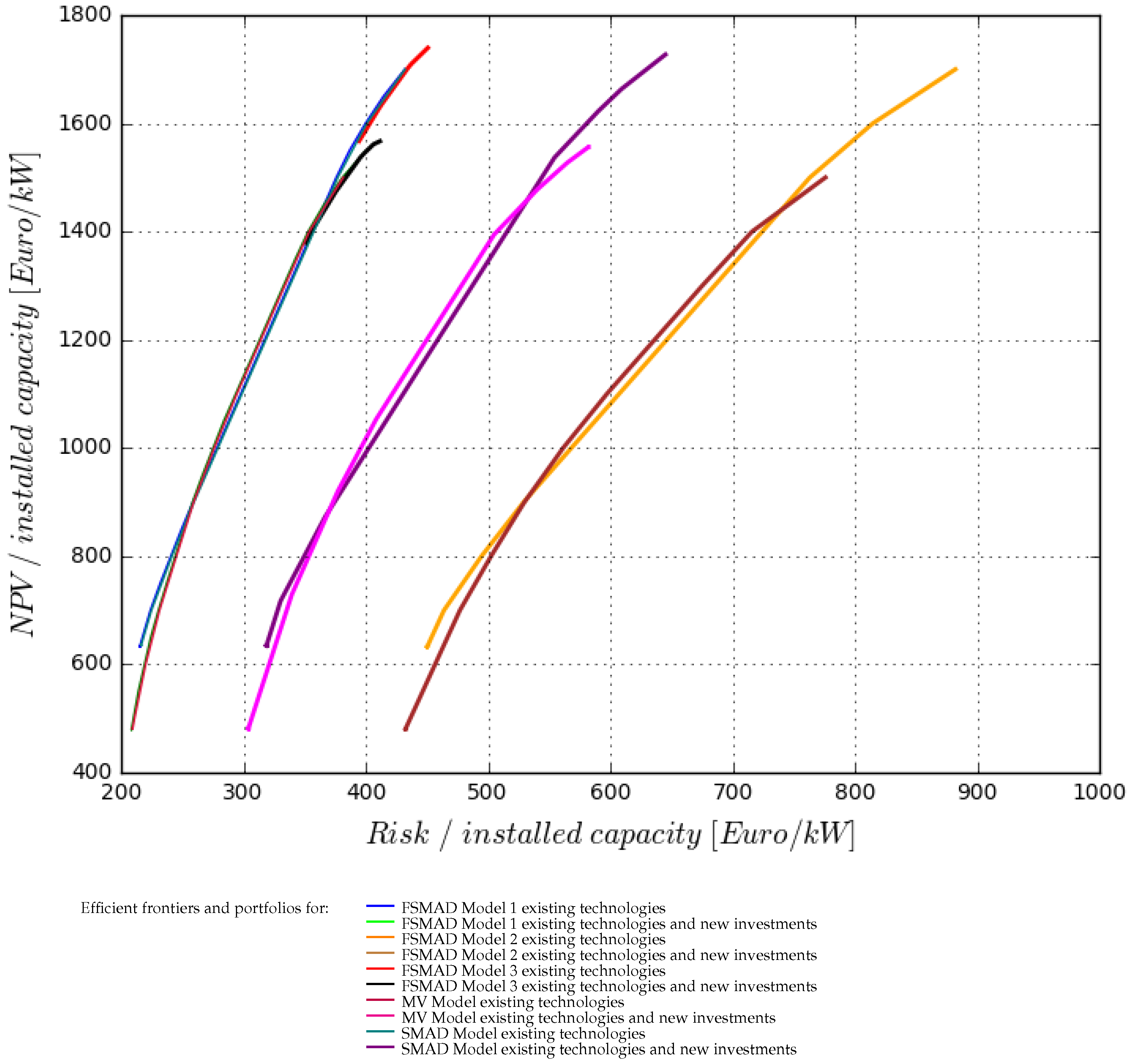
Figure 3 presents the location of the efficient frontiers for the FSMAD models described in Section 3, together with the SMAD Model and the MV Model (analogously to the other presented models and their efficient frontiers, tables with the technology shares in the efficient power generation mixes for the MV Model are presented in

Table A7. Efficient portfolios according to the MV Model for existing technologies.

	Efficient Portfolios
Technologies	P1	P2	P3	P4	P5	P6
Biomass	0.07%	0.07%	0.07%	0.07%	0.07%	0.07%
CCGT	9.19%	9.19%	0.00%	0.00%	0.01%	9.19%
CHP	8.53%	8.53%	8.53%	8.53%	8.53%	0.00%
GT gas	3.24%	3.24%	3.24%	0.00%	0.00%	0.00%
GT oil	7.24%	7.24%	7.24%	7.24%	0.00%	0.00%
Hard coal	45.67%	45.67%	45.67%	7.72%	14.96%	14.03%
Hydro	14.95%	14.95%	14.95%	14.95%	14.95%	14.95%
Lignite	8.22%	0.00%	0.00%	8.22%	8.22%	8.22%
Nuclear	2.46%	10.68%	19.87%	52.84%	52.84%	52.84%
Onshore	0.42%	0.42%	0.42%	0.42%	0.42%	0.42%
NPV [€/kW]	634.86	717.45	872.77	1622.72	1663.38	1727.25
Risk [€/kW]	318.89	330.45	366.85	590.29	609.14	645.13

and

Table A8. Efficient portfolios according to the MV Model for existing technologies combined with new investments.

	Efficient Portfolios
Technologies	P1	P2	P3	P4	P5	P6	P7
Biomass	0.06%	0.06%	0.06%	0.06%	0.06%	0.06%	0.06%
CCGT	16.36%	16.36%	7.83%	0.00%	0.00%	7.83%	7.83%
CHP	7.26%	7.26%	7.26%	7.26%	7.26%	7.26%	0.00%
GT gas	2.76%	2.76%	2.76%	2.76%	0.00%	0.00%	0.00%
GT oil	6.17%	6.17%	6.17%	6.17%	4.29%	0.00%	0.00%
Hard coal	48.76%	38.88%	38.88%	38.88%	19.56%	16.03%	23.29%
Hydro	12.73%	12.73%	12.73%	12.73%	12.73%	12.73%	12.73%
Lignite	1.79%	0.00%	0.00%	0.00%	7.00%	7.00%	7.00%
Nuclear	0.00%	11.67%	20.20%	28.03%	44.98%	44.98%	44.98%
Offshore	3.76%	3.76%	3.76%	3.76%	3.76%	3.76%	3.76%
Onshore	0.36%	0.36%	0.36%	0.36%	0.36%	0.36%	0.36%
NPV [€/kW]	481.70	729.34	920.59	1052.80	1477.83	1527.36	1556.31
Risk [€/kW]	304.10	339.65	377.32	408.49	540.34	564.89	582.19

in the Appendix A). The position of the MV efficient frontier, in contrast to the SMAD Model as well as FSMAD Models 1 and 3, shows the shift in the scale of risk. These two fuzzy models (FSMAD Models 1 and 3) and the semi-mean-absolute deviation model perform better. They achieve a smaller expected risk for the same return level than the other models presented (see also Table 1). Further interesting results observed are the higher gradients of the efficient frontiers for the SMAD Model as well for FSMAD Models 1 and 3, in comparison to the efficient frontiers obtained with the MV Model and FSMAD Model 2, respectively.

Analyzing the comparison of the risk levels for the given portfolio return values (Table 1), it can be noticed that FSMAD Model 2 performs the worst in comparison to all other models. The membership function applied in this model has a trapezoidal form like that in FSMAD Model 1, but a different tolerance interval and left- and right-width parameters (see Section 3.2). The introduction of sufficiency and necessity return and risk levels in FSMAD Model 3 have the effect that the efficient frontier is shorter in comparison to those of the other models (see Figure 1c), and the risk values for smaller portfolio returns are inexistent (see Table 1).

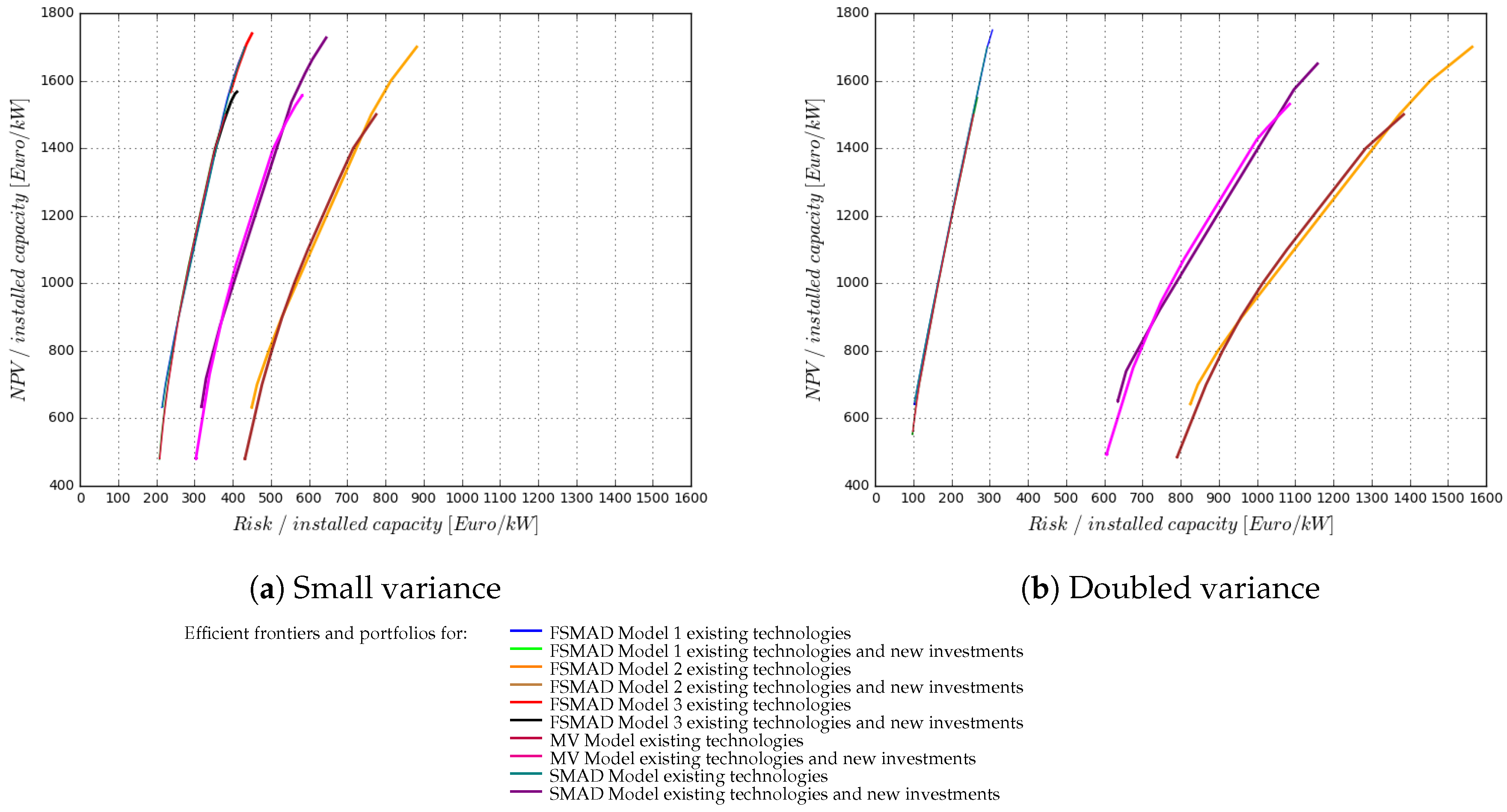
In the following, we compare the results presented in Figure 3 with portfolios obtained when the distribution parameters, especially the variance of the commodities considered in the calculation of the expected returns of the power generation portfolio assets, change. In order to mimick more downside and upside events, we doubled the variance and re-simulated the return values for all considered technologies. Simulation results were applied to the portfolio selection based on the all models presented in the paper. Figure 4 compares the location of efficient frontiers obtained previously—plot (a) (the graphic is similar to Figure 3 but the scale of the risk is changed for better comparison) with efficient frontiers obtained when doubling the variance—plot (b). As can be seen, the efficient frontier for the MV portfolio selection model shifts markedly to the right, implying that portfolios are characterized with higher risk for the same expected return in comparison to the previous situation. In contrast, the efficient portfolios obtained according to FSMAD Model 1 and the SMAD Model shift only slightly to the left. This observation proves the previously mentioned property of the SMAD Model, i.e., that the SMAD as a risk measure is less sensitive to outliers and equivalent to the MV approach. The efficient frontier obtained for FSMAD Model 2 also shifts strongly to the right, which can be a consequence of the membership function applied in this model (i.e. one which uses the quantiles, which is the cause of large variance change, too).

Table 2. Risk values for all models for selected portfolio returns, doubled variance [both in €/kW].

Value of the	Model
Portfolio Return	FSMAD 1	FSMAD 2	FSMAD 3	MV	SMAD
(a) Existing technologies
650	104.14	826.08	-	635.87	104.54
850	137.77	960.56	-	746.05	138.18
1750	307.61	1563.66	8760.03	1159.59	308.59
(b) Existing technologies and new investments
600	103.21	931.59	-	611.38	102.96
1050	174.99	831.59	-	810.16	173.49
1550	268.18	1384.35	7958.00	1085.83	267.73

compares the risk levels obtained for the given portfolio return values when the variance is doubled. In the case of FSMAD Model 1 and the SMAD Model, the risk value decreases slightly in comparison to the previous situation presented in Table 1 (compare also the shift of the efficient frontiers in Figure 4). For the FSMAD Model 2 as well as the MV Model, the portfolio risk increases strongly. The most interesting result, however, can be observed for FSMAD Model 3, where the risk value increased most (see Table 2), and where the investor’s aspiration levels regarding risk and return were included. As mentioned in Section 3.2, these levels can be defined by the decision-makers and also calculated using mathematical methods, such as those proposed by [41] and used in our case. Hence, the efficient frontier for this portfolio selection model is not presented in Figure 4b.

5. Conclusions

In this paper, we have presented several alternative portfolio selection models for power generation assets based on fuzzy sets theory and semi-mean-absolute deviation as a risk measure. On the one hand, the use of another risk measure than the standard deviation (as it is used in the standard Markowitz model) was already suggested by Markowitz himself, but the first application only emerged in the aftermath of post-modern portfolio theory. On the other hand, measures such as the semi-variance or semi-absolute deviation, from an investor’s point of view, describe the expected losses and thus the part of the risk (the downside risk) that really matters risk. For this reason, the consideration of these measures in decision-making processes seems to be necessary, or even indispensable. In the presented results, the use of the SMAD Model caused a shift of the efficient frontier along the risk axis. More precisely, the efficient portfolios for the same return level have a smaller risk than portfolios obtained with the MV Model. For a decision-maker with risk aversion, such a shift can positively affect the decision-making outcome.

The analysis carried out in this paper illustrates the application possibilities of fuzzy portfolio selection models for power generation assets. Specifically, introducing membership functions for the description of investors’ aspiration levels for the expected return and risk (FSMAD Model 3) shows how the knowledge of experts, and an investor’s subjective opinions, can be better integrated into the decision-making process. In the cases presented, we have shown that using one of these models affects the size of the set of efficient portfolios (the set is smaller than when using FSMAD, SMAD or MV models). The sparse set of alternatives, which is considered in the decision-making process, can push on and relieve this process. Moreover, in FSMAD Model 3, the decision-maker can help to exactly determine the so-called sufficiency and necessity levels and obtain the optimal solution.

The fuzzy portfolio selection models and the model that uses the semi-mean-absolute deviation as a risk measure presented in this paper illustrated their application for energy utilities, just as they exist for other industries and the financial markets. The complexity of the energy markets, the uncertain environment, the vagueness or some other type of fuzziness, can overall be better captured with fuzzy sets theory. However, the further development of these models especially for the energy sector is required, which calls for more research in this field as well as applications of other alternative risk measures, such as, e.g., the CVaR.

References

- Markowitz, H. Portfolio Selection. J. Financ. 1952, 7, 77–91. [Google Scholar]
- Konno, H.; Yamazaki, H. Mean-absolute deviation portfolio optimization model and its application to Tokyo stock market. Manag. Sci. 1991, 37, 519–531. [Google Scholar] [CrossRef]
- Konno, H.; Koshizuka, T. Mean-absolute deviation model. IIE Trans. 2005, 25, 893–900. [Google Scholar] [CrossRef]
- Mansini, R.; Speranza, M. A Heuristic Algorithm for a Portfolio Selection Problem with Minimum Transaction Lots. Eur. J. Oper. Res. 1999, 114, 219–223. [Google Scholar] [CrossRef]
- De Silva, L.; Alem, D.; de Carvalho, F. Portfolio optimization using Mean Absolute Deviation (MAD) and Conditional Value-at-Risk (CVaR). Production 2017, 27, 1–14. [Google Scholar] [CrossRef]
- Liu, S. The mean-absolute deviation portfolio selection problem with interval-valued returns. J. Comput. Appl. Math. 2011, 235, 4149–4157. [Google Scholar] [CrossRef]
- Mansini, R.; Ograczyk, W.; Sparanza, M. Twenty years of linear programming based portfolio optimization. Eur. J. Oper. Res. 2014, 234, 518–535. [Google Scholar] [CrossRef]
- Zimmermann, H. Fuzzy Set Theory and Its Applications; Kluwer Academic Publishers: Dordrecht, The Netherlands, 2001. [Google Scholar]
- Zadeh, L. Fuzzy sets. Inf. Control 1965, 8, 338–353. [Google Scholar] [CrossRef] [Green Version]
- Zadeh, L. Fuzzy sets as a basis for a theory of possibility. Fuzzy Sets Syst. 1978, 1, 3–28. [Google Scholar] [CrossRef]
- Dubois, D.; Prade, H. Possibility Theory; Plenum Press: New York, NY, USA, 1988. [Google Scholar]
- Bellman, R.; Zadeh, L. Decision-making in a fuzzy environment. Manag. Sci. 1970, 17, 141–164. [Google Scholar] [CrossRef]
- Fang, Y.; Lai, K.; Wang, S. Fuzzy Portfolio Optimization: Theory and Methods; Springer: Berlin/Heidelberg, Germany; New York, NY, USA, 2008. [Google Scholar]
- Wang, S.; Zhu, S. On Fuzzy Portfolio Selection Problem. Fuzzy Optim. Decis. Mak. 2002, 1, 361–377. [Google Scholar] [CrossRef]
- Watada, J. Fuzzy Portfolio Selection and its Applications to Decision Making. Tatra Mt. Math. Publ. 1997, 13, 219–248. [Google Scholar]
- Tanaka, H.; Guo, P. Portfolio selection based on upper and lower exponential possibility distribution. Eur. J. Oper. Res. 1999, 114, 115–126. [Google Scholar] [CrossRef]
- Bar-Lev, D.; Katz, S. A Portfolio Approach to Fossil Fuel Procurement in the Electric Utility Industry. J. Financ. 1976, 31, 933–947. [Google Scholar] [CrossRef]
- Madlener, R. Portfolio Optimization of Power Generation Assets. In Handbook of CO2 in Power Systems; Zheng, Q., Rebennack, S., Pardalos, P., Pereira, M., Iliadis, N., Eds.; Springer: Berlin/Heidelberg, Germany; New York, NY, USA, 2012; pp. 275–296. [Google Scholar]
- Awerbuch, S.; Berger, M. Applying Portfolio Theory to EU Electricity Planning and Policy-Making; OECD/IEA: Paris, France, 2003. [Google Scholar]
- Roques, F.; Newbery, D.; Nuttall, W. Fuel mix diversification in liberalized electricity markets: A mean- variance portfolio theory approach. Energy Econ. 2007, 30, 1831–1849. [Google Scholar] [CrossRef]
- Krey, B.; Zweifel, P. Efficient and secure power for the United States and Switzerland. In Analytical Methods for Energy Diversity and Security: Portfolio Optimization in the Energy Sector: A Tribute to the Work of Dr. Shimon Awerbuch; Bazilian, M., Roques, F., Eds.; Elsevier: New York, NY, USA, 2008; pp. 193–218. [Google Scholar]
- Madlener, R.; Wenk, C. Efficient Investment Portfolios for the Swiss Electricity Supply Sector; FCN Working Paper No. 2/2008; Institute for Future Energy Consumer Needs and Behavior, Faculty of Business and Economics/E.ON Energy Research Center, RWTH Aachen University: Aachen, Germany, August 2008. [Google Scholar]
- Borchert, J.; Schemm, R. Einsatz der Portfoliotheorie im Asset Allokations-Prozess am Beispiel eines fiktiven Anlageraums von Windkraftstandorten. Z. Energiewirtsch. 2007, 31, 311–322. [Google Scholar]
- Glensk, B.; Ganczarek-Gamrot, A.; Trzpiot, G. Portfolio Analysis on Polish Power Exchange and European Energy Exchange. In Multiple Criteria Decision Making; Konczak, G., Michnik, J., Nowak, M., Trzaskalik, T., Wachowicz, T., Eds.; UE Katowice: Katowice, Poland, 2013; Volume 8, pp. 18–29. [Google Scholar]
- Sharpe, W. Capital Asset Prices: A Theory of Market Equilibrium under Considerations of Risk. J. Financ. 1964, XIX, 425–442. [Google Scholar]
- Konno, H. Piecewise linear risk function and portfolio optimization. J. Oper. Res. 1990, 33, 139–156. [Google Scholar] [CrossRef]
- Bower, B.; Wentz, P. Portfolio Optimization: MAD vs. Markowitz. Rose-Hulm. Undergrad. Math. J. 2005, 6, 1–17. [Google Scholar]
- Artzner, P.; Delbaen, F.; Eber, J.M.; Heath, D. Coherent measures of risk. Math. Financ. 1999, 9, 203–228. [Google Scholar] [CrossRef]
- Föllmer, H.; Schied, A. Stochastic Finance: An Introduction in Discrete Time; Walter de Gruyter: Berlin, Germany, 2002. [Google Scholar]
- Pflug, G.; Romisch, W. Modeling, Measuring and Managing Risk; World Scientific Publishing: Singapore, 2007. [Google Scholar]
- Rockafellar, R.; Uryasev, S.; Zabarankin, M. Generalized deviation in risk analysis. Financ. Stoch. 2006, 10, 51–74. [Google Scholar] [CrossRef]
- Rockafellar, R.; Uryasev, S.; Zabarankin, M. Optimality conditions in portfolio analysis with general deviation measures. Math. Program. 108 2006, 2–3, 515–540. [Google Scholar] [CrossRef]
- Ogryczak, W.; Ruszczynski, A. From stochastic dominace to mean-risk models: Semideviations as risk measures. Eur. J. Oper. Res. 1999, 116, 33–50. [Google Scholar] [CrossRef]
- Mansini, R.; Ograczyk, W.; Sparanza, M. Solvable Models for Portfolio Optimization: A Classification and Computational Comparison. IMA J. Manag. Math. 2003, 14, 187–220. [Google Scholar] [CrossRef]
- Speranza, M. A Heuristic Algorithm for a Portfolio Optimization Model applied to the Milan stock Market. Comput. Oper. Res. 1996, 23, 433–441. [Google Scholar] [CrossRef]
- Carlsson, C.; Fullér, R. On possibilistic mean value and variance of fuzzy numbers. Fuzzy Sets Syst. 2001, 122, 315–326. [Google Scholar] [CrossRef] [Green Version]
- Carlsson, C.; Fullér, R.; Majlender, P. A possibilistic approach to selecting portfolios with highest utility score. Fuzzy Sets Syst. 2002, 131, 13–21. [Google Scholar] [CrossRef] [Green Version]
- Vercher, E.; Bermudez, J.; Segura, J. Fuzzy portfolio optimization under downside risk measures. Fuzzy Sets Syst. 2007, 158, 769–782. [Google Scholar] [CrossRef] [Green Version]
- Huang, X. Portfolio selection with fuzzy returns. J. Intell. Fuzzy Syst. 2007, 18, 383–390. [Google Scholar]
- Chen, G.; Liao, X. A possibilistic Mean Absolute Deviation Portfolio Selection Model. In Fuzzy Information and Engineering; Cao, B., Zhang, C., Eds.; Springer: Berlin/Heidelberg, Germany; New York, NY, USA, 2009. [Google Scholar]
- Zimmermann, H. Fuzzy programming and linear programming with several objective functions. Fuzzy Sets Syst. 1978, 1, 45–55. [Google Scholar] [CrossRef]
- Vasant, P. Fuzzy production planning and its application to decision making. J. Intell. Manuf. 2006, 17, 5–12. [Google Scholar] [CrossRef]
- Madlener, R.; Glensk, B.; Weber, V. Fuzzy Portfolio Optimization of Onshore Wind Power Plants; FCN Working Paper No. 10/2011; Institute for Future Energy Consumer Needs and Behavior, Faculty of Business and Economics/E.ON Energy Research Center, RWTH Aachen University: Aachen, Germany, May 2011. [Google Scholar]
- Madlener, R.; Glensk, B.; Raymond, P. Investigation of E.ON’s Power Generation Assets by Using Mean-Variance Portfolio Analysis; FCN Working Paper No. 12/2009; Institute for Future Energy Consumer Needs and Behavior, Faculty of Business and Economics/E.ON Energy Research Center, RWTH Aachen University: Aachen, Germany, November 2009. [Google Scholar]
- Brigham, E.; Ehrhardt, M. Financial Management: Theory and Practice; South-Western CENGAGE Learning: Mason, OH, USA, 2008. [Google Scholar]
- Madlener, R.; Glensk, B. Portfolio Impact of New Power Generation Investments of E.ON in Germany, Sweden and the UK; FCN Working Paper No. 17/2010; Institute for Future Energy Consumer Needs and Behavior, Faculty of Business and Economics/E.ON Energy Research Center, RWTH Aachen University: Aachen, Germany, November 2010. [Google Scholar]
Figure 1.
Efficient frontiers obtained for different FSMAD models.
Figure 2.
Comparison of efficient frontiers obtained with the FSMAD Model 1 and the SMAD Model.
Figure 3.
Comparison of the efficient frontiers obtained with all models considered.
Figure 4.