Robust Load Frequency Control Schemes in Power System Using Optimized PID and Model Predictive Controllers
by
 , , and
Komboigo Charles
1,* ,
,
Naomitsu Urasaki
1,
Tomonobu Senjyu
1 ,
,
Mohammed Elsayed Lotfy
1,2 and
Lei Liu
1 1
Electrical and Electronics Engineering Department, University of the Ryukyus, Okinawa 903-0213, Japan
2
Electrical Power and Machines Department, Zagazig University, Zagazig 44519, Egypt
*
Author to whom correspondence should be addressed.
Energies 2018, 11(11), 3070; https://doi.org/10.3390/en11113070
Submission received: 16 October 2018
/
Revised: 30 October 2018
/
Accepted: 5 November 2018
/
Published: 7 November 2018
(This article belongs to the Special Issue Electric Power Systems Research 2018)
Abstract
:Robust control methodology for two-area load frequency control model is proposed in this paper. The paper presents a comparative study between the performance of model predictive controller (MPC) and optimized proportional–integral–derivative (PID) controller on different systems. An objective function derived from settling time, percentage overshoot and percentage undershoot is minimized to obtain the gains of the PID controller. Genetic Algorithm (GA) and Particle Swarm Optimization (PSO) are used to tune the parameters of the PID controller through performance optimization of the system. System performance characteristics were compared to another controller designed based on MPC. Detailed comparison was performed between the performances of the MPC and optimized PID. The effectiveness and robustness of the proposed schemes were verified by the numerical simulation in MATLAB environment under different scenarios such as load and parameters variations. Moreover, the pole-zero map of each proposed approach is presented to investigate their stability.
1. Introduction
Load frequency control (LFC) is used to regulate the power output of the electric generator within an area as the response of changes in system frequency and tie-line loading. Thus, LFC helps in maintaining the scheduled system frequency and tie-line power interchange with the other areas within the prescribed limits. Studies on frequency control approaches for the hybrid power system using fuzzy logic control (FLC) [1,2], -synthesis scheme [3], H∞ and -synthesis approach [4], neuro-fuzzy control [5], FLC with the particle swarm optimization (PSO) algorithm implementation [6,7], FLC with chaotic PSO [8], -MOGA [9], PSO with mixed H/H∞ control [10], the quasi-oppositional harmony search algorithm (QOHSA) [11], sliding mode control (SMC) [12], multiple model predictive control (MMPC) [13], multi-variable generalized predictive control (MGPC) [14] and Type-2 FLC with the modified harmony search algorithm (MHSA) [15] have been carried out with promising results. However, this control approach tries to damp frequency and tie-line power deviations to eliminate the drawbacks related to most of the previous schemes such as H∞ and FLC techniques. The weighting functions in the H∞ design process cannot be chosen in an easy way. This action affects dramatically the design process. Moreover, the H∞ controller order is the same as that of the plant. This produces a complicated frame which is not easy to be implemented especially for large systems. Moreover, accurate and sufficient knowledge base affects greatly the impact of the FLC scheme. Increasing the number of rules in the knowledge base leads to increase complexity, which in turn affects the computational time and requirements of memory [16]. Comparing MPC controller to conventional PID controller, it is worth mentioning that MPC consumes extra time for on-line computations when the constraints intervene. Parameters of MPC are designed based on successive iterations, where no mathematical forms have been developed yet to determine the best configuration of the parameters. A large volume of literature considers performance comparison between MPC and conventional PID control, where the results usually point out to noticeable MPC superiority [17,18]. MPC is also used in renewable energy sources control [19,20]. In this research, a comparison between the performances of MPC and optimized PID controllers is presented using different performance indices. To guarantee a fair comparison, the PID controller parameters are optimized by using genetic algorithm and particle swarm optimization. The performance of the proposed method is investigated for the two-area interconnected power systems. The results are tabulated as a comparative performance in view of peak overshoot, peak undershoot, settling time and the capability of the proposed algorithm to solve LFC problem under different disturbances is confirmed. The main contributions of this research can be summarized as follows:
- This study presents a complete load frequency control scheme using optimized PID and model predictive controllers.
- The robustness of the proposed control approaches are investigated against system parameters variations.
- The nonlinear governor time delay is considered to confirm the ability of the proposed control techniques for practical implementation.
- Pole zero maps for each control loop are investigated to ensure the stability of each control method and its capability to be applied over wide range of operating conditions.
This paper is divided into seven sections. Section 1 comprises this Introduction. Section 2 presents the system dynamics. Section 3 illustrates the model predictive controller. Section 4 presents optimized proportional–integral–derivative controller. Section 5 discusses the genetic algorithm and particle swarm optimization. Section 6 focuses on the simulations and discussion of the results. A comparative study is also presented in this section. Finally, the last section is devoted to the conclusion of this paper.
2. System Dynamics
In this section, a simplified frequency response model for two area power system with an aggregated generator unit is described in Figure 1 and Figure 2 while the parameters of the system are presented in Table 1.
The dynamic model in state variation form can be obtained from the function model and is given by:
where , , , are constant matrices, is the state vector, and is the control vector.
2.1. Model Predictive Controller
In Figure 1, the governor, turbine and power system of every area are represented by first order transfer function. For , i = . The input of MPC is chosen to be Area Control Error (ACE), where = + , i = while the output of MPC is the control signal.
2.1.1. For MPC1
2.1.2. For MPC2
2.2. Optimized PID Controller
In Figure 2, governor, turbine and power system are still represented by first order transfer function. Every PID controller is divided into (I) and (P + D) controllers, as shown in the figure, and the integral of (ACE) for each area is considered as state to perform the state space model.
where
where, and are frequency deviations in Areas 1 and 2 (pu Hz), is the tie line power deviation in the two-area system (pu MW), and are load disturbances in Areas 1 and 2 (pu MW), and are power system time constants in Areas 1 and 2, and are turbine time constants in Areas 1 and 2, and are governor time constants in Areas 1 and 2, and are power system constants in Areas 1 and 2, and are tie line frequency biases in Areas 1 and 2, and are regulations of governors in Areas 1 and 2, is the synchronizing coefficients for tie lines for the two-area system, and and are area control errors in Areas 1 and 2.
3. Model Predictive Control
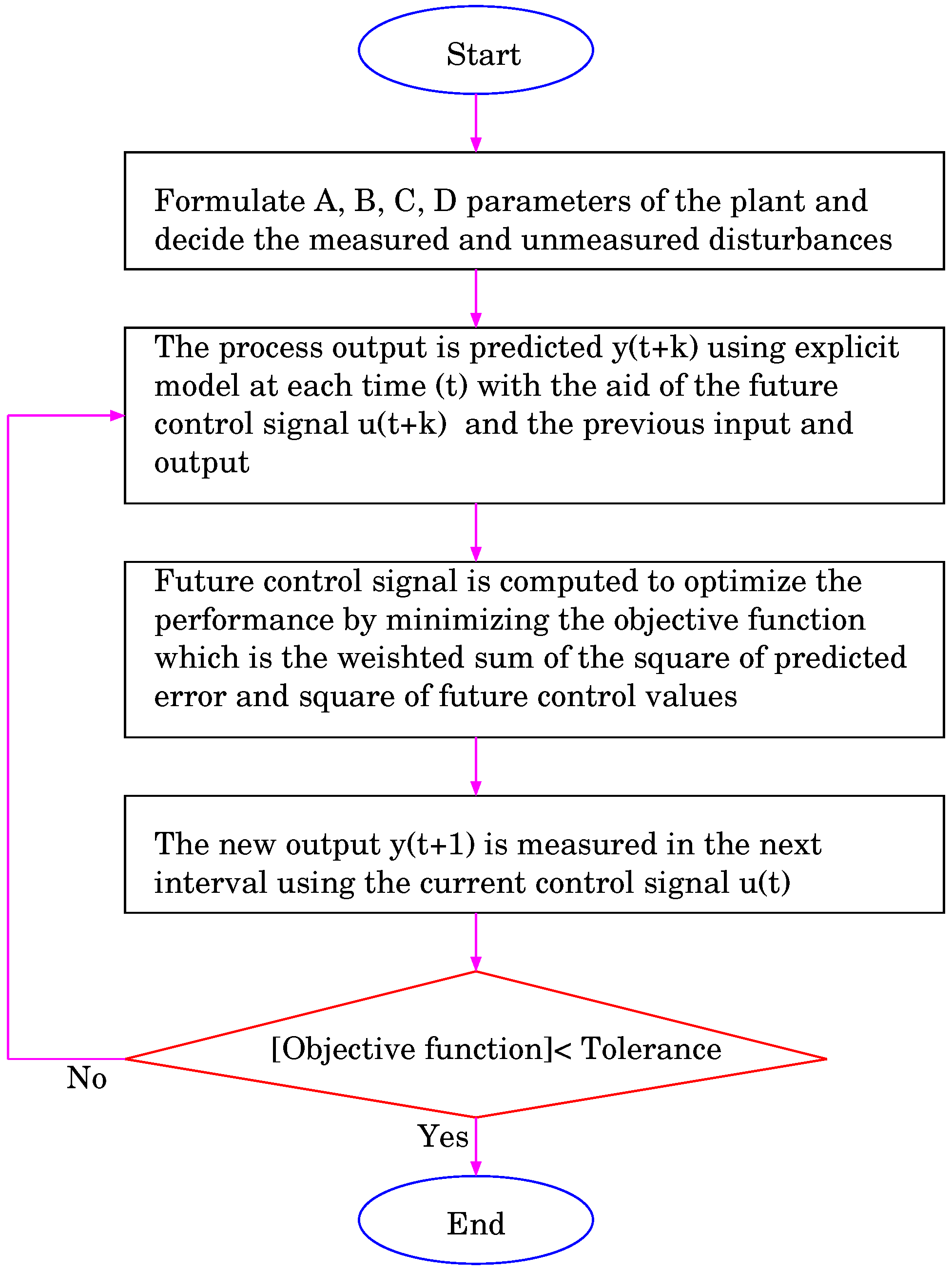
MPC is a novel control approach that can be used to control wide range of industrial applications. Multi-input multi-output systems, linear and nonlinear systems and even constrained systems are among these applications. The superiority of MPC exists in it stability to estimate the future performance of the plant using adaptive optimization scheme. The main configuration of MPC is presented in Figure 3 while the main process of MPC can be summarized in the following steps, which are indicated in Figure 4.
- Future time horizon is used to predict the process output utilizing an explicit model at each time (t). The predicted output , …, N can be calculated using the future control signal, , …, N − 1 and the previous inputs and outputs.
- A chain of future control signals is computed to optimize a performance criterion by minimizing an objective function. The objective function to be mitigated is a weighted summation for the square of predicted errors and square of future control values.where and are weighting factors, and are the lower and upper prediction horizons over the output, and is the control horizon. The number of future control can be decreased using the control horizon by the following equations:
- is measured at the next interval using the current control signal , and then Step 1 is repeated to get . As a result, the horizon is shifted at each interval by the same length.
The main steps of MPC are formulated as a flowchart in Figure 5.
4. Optimized PID Controller Using Genetic Algorithm and Particle Swarm Optimization
The control signal of a continuous PID controller is given as.
where is the controller output, , and are the PID controller gains, and is the mismatch between reference and actual output values. To guarantee a fair comparison between MPC and PID controllers, the PID controller parameters , and are optimized using Genetic Algorithm (GA) and Particle Swarm Optimization (PSO). Genetic Algorithm and Particle Swarm Optimization are considered as the most utilized optimization techniques. They have the ability to solve linear and nonlinear optimization problems [21].
4.1. Genetic Algorithm (GA)
GA, a technique for solving constrained and unconstrained optimization problems, is based on natural selection, the process that drives biological evolution. A key step in GA applications is the definition of the objective (fitness) function, which is the function we want to optimize. Here, the fitness function is taken to minimize the sum squared error of frequency of Area 1, Area 2 and tie power.
Genetic Algorithm tries to utilize the current generation to get new population. GA tries to choose the best individuals of the current population that has best fitness value called parents, and use them to get the individuals of the upcoming generation called children. Every generation, GA is used to make three categories of children for the upcoming population:
- The individuals who have the best fitness value in this generation are passed directly to the next generation and called elite individuals.
- Some children are created by combining two parents who have good fitness value and are called crossover children.
- Some other children are subjected random changes and are called mutation children.
4.2. Particle Swarm Optimization (PSO)
PSO algorithm is a new approach based on the movement and intelligence of swarms. This method was developed by James Kennedy and Russell Eberhart as an optimization techniques in 1995 [21]. Particles are utilized to move in the search space searching for the solutions that have best values. The flying of each particle is adjusted according to its own flying history and also other particles flying experience. Unlike in genetic algorithms, evolutionary programming and evolutionary strategies, in PSO, there is no selection operation. All particles in PSO are kept as population members through the track of the run. PSO is the only algorithm that does not implement survival of the fittest. This computational technique was inspired by social behavior of birds flocking or fish schooling. In this technique, a group of random particles (solutions) is generated. According to fitness value, the best solution is determined in the current iteration and also the best fitness value is stored. The best solution is known as pbest. Another best fitness value is also tracked in the iterations obtained thus far. This best fitness value is a global best and its corresponding particle (solution) is called gbest. In every iteration, all particles will be updated by following the best previous position (pbest) and best particle among all the particles ( gbest) in the swarm. Here, the fitness function is taken to minimize the sum squared error of frequency of Area 1, Area 2, and tie power.
The flowchart of the main steps of PSO is presented in Figure 6.
5. Simulation Results and Comparison
This section presents the simulation results of the proposed approach MPC controller and optimized PID controller on different systems. Two-area interconnected power systems were considered for the simulation. The two-area interconnected systems shown in Figure 1 and Figure 2 were simulated for 0.2 pu step load perturbation in Area 1 and no load disturbance in Area 2. The optimized values of GA-PID, PSO-PID and parameters are presented in Table 2.
5.1. MPC Parameters
- Prediction horizon = 10
- Control horizon = 2.00
- Weights on manipulated variable = 0.80
- Weights on manipulated variable rates = 0.10
- Weights on the output signals = 0.10
5.2. GA-PID Fitness Function
The GA is used to find the best , , and values for the PID controller. The parameter values tuned for GA algorithm are:
- Population size = 200
- Initial range = [0.5;1]
- Elite count = 2.00
- Crossover = 0.80
- Mutation = 0.20
5.3. PSO-PID Fitness Function
The PSO is used to find the best , , and values for the PID controller. The parameter values tuned for PSO algorithm are:
- Population size = 300
- Inertia weight w = 1.00
- Cognitive coefficient C1 = 1.50
- Social coefficient C2 = 2.00
5.4. Cases Study
To investigate the robustness and effectiveness of the proposed controllers, the two-area interconnected power systems were subjected to four different operating conditions.
5.4.1. First Case
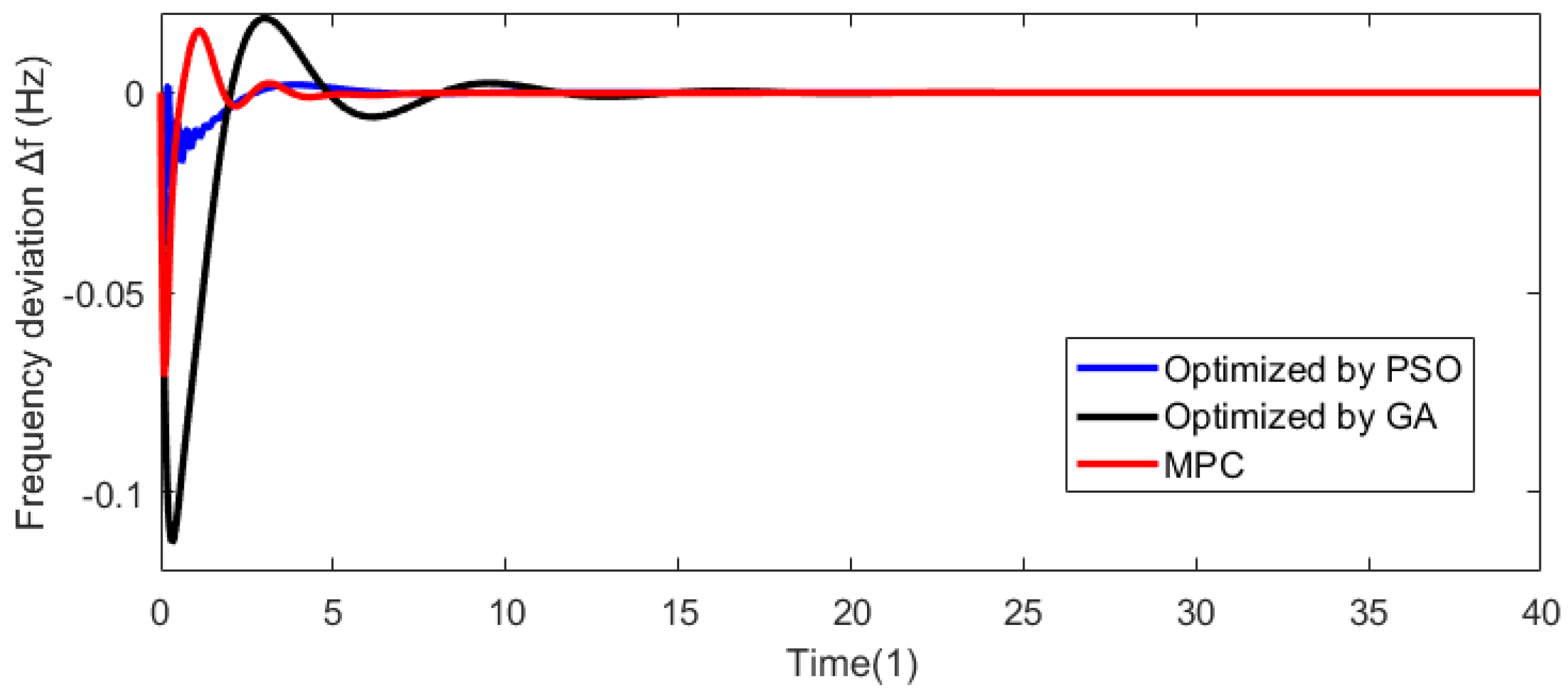
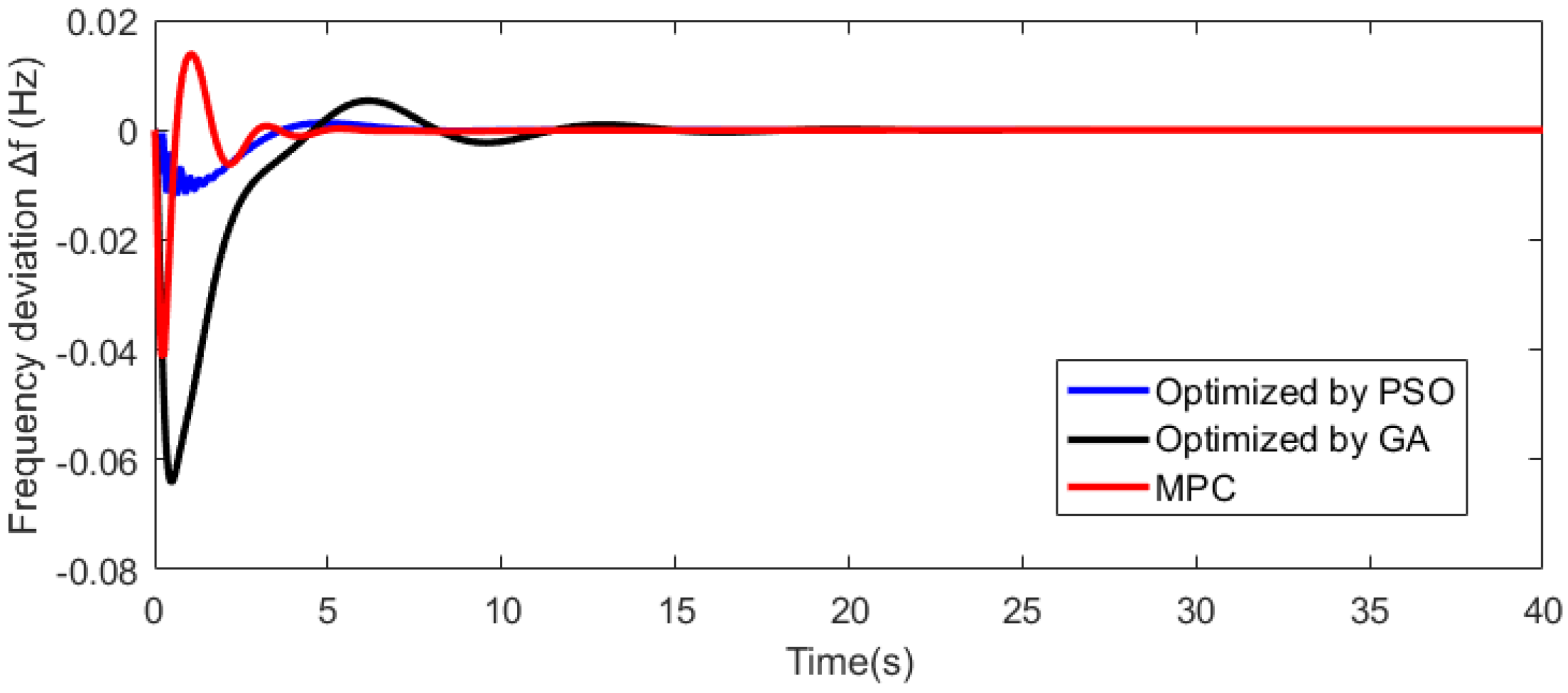
The first condition was achieved by implementing the two-area power system using nominal values of their parameters, as shown in Figure 7, Figure 8 and Figure 9. Figure 7 shows the frequency deviation in Area 1 for the first case, Figure 8 shows the frequency deviation in Area 2 for the first case, and Figure 9 presents the tie line power deviation for the first case.
5.4.2. Second Case
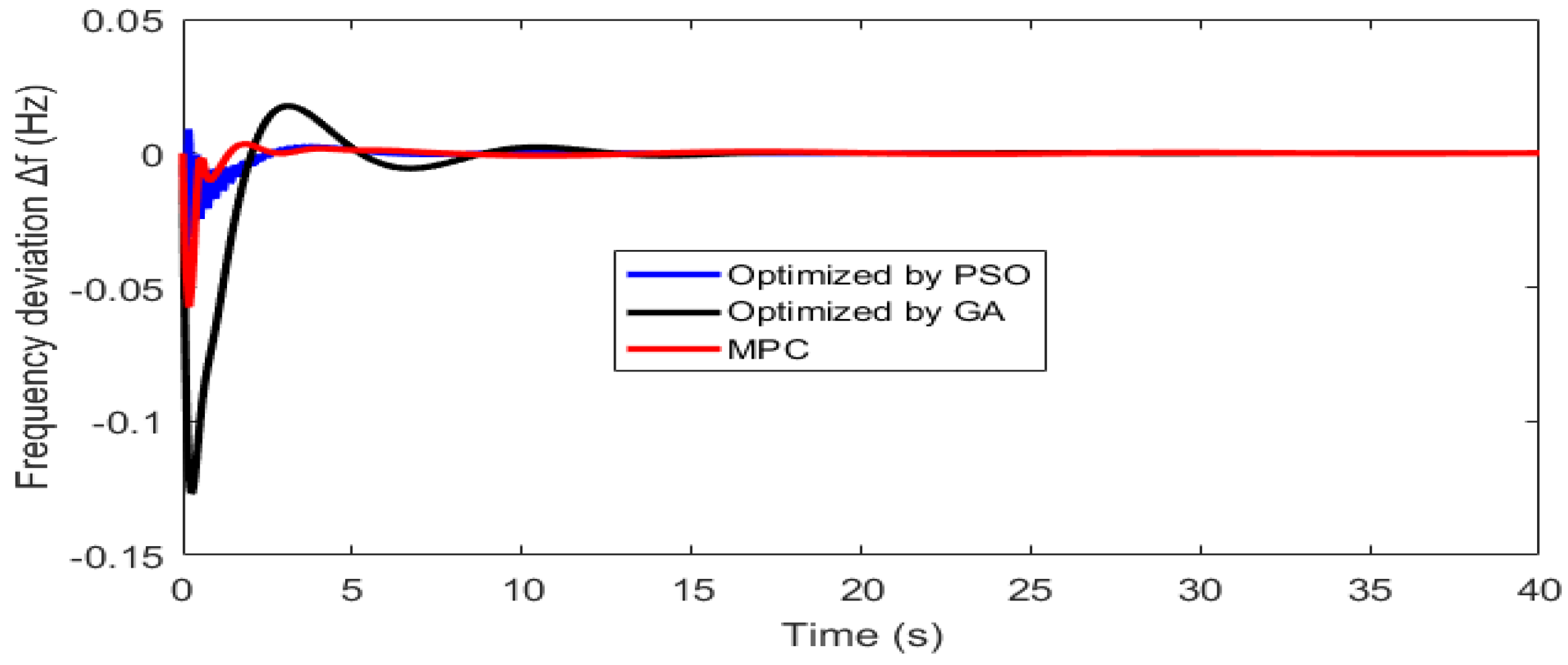
The second condition was achieved by implementing the two-area power system by modifying the plant gains and at percent of its nominal value. The performance of the proposed approaches is clarified in Figure 10, Figure 11 and Figure 12. Figure 10 shows the frequency deviation in Area 1 for the second case, Figure 11 shows the frequency deviation in Area 2 for the second case and Figure 12 presents the tie line power deviation for the second case.
5.4.3. Third Case
The third condition was achieved by implementing the two-area power system by modifying the synchronizing coefficients for the tie-line at percent of its nominal value. The performance of the proposed approaches is clarified in Figure 13, Figure 14 and Figure 15. Figure 13 shows the frequency deviation in Area 1 for the third case, Figure 14 shows the frequency deviation in Area 2 for the third case and Figure 15 presents the tie line power deviation for the third case. Detailed analysis for the three scenarios comparing the performance of the proposed control schemes is presented in the following subsection. It is worth mentioning that and were chosen because they are the most sensitive parameters in the system, i.e. the response of the power system is very sensitive to changes in their values.
5.4.4. Fourth Case
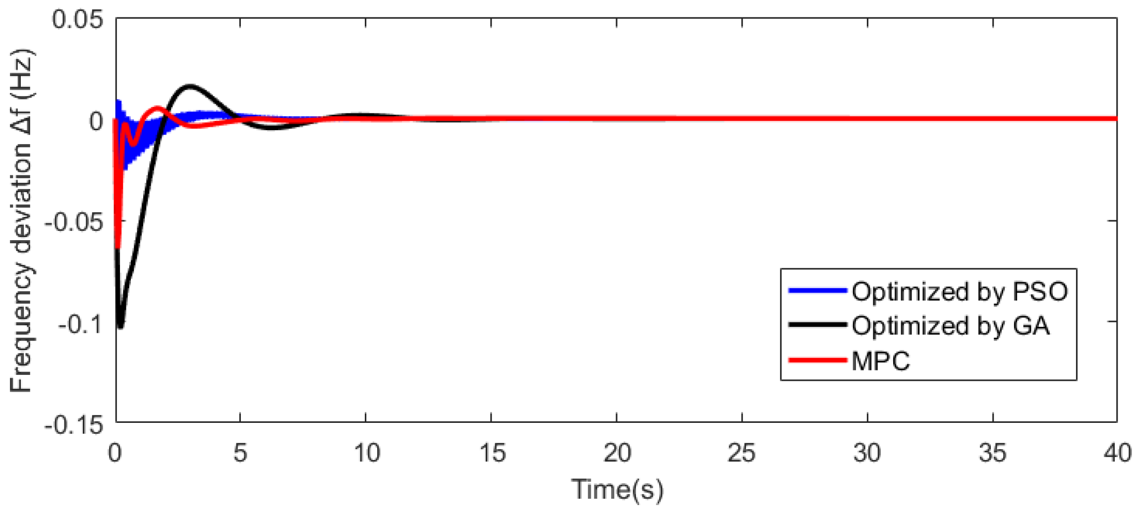
The fourth condition was achieved by implementing the two-area power system by taking consideration of the turbine time delay. The performance of the proposed approaches is clarified in Figure 16, Figure 17 and Figure 18. Figure 16 shows the frequency deviation in Area 1 for the fourth case, Figure 17 shows the frequency deviation in Area 2 for the fourth case and Figure 18 presents the tie line power deviation for the third case. Detailed analysis for the three scenarios comparing the performance of the proposed control schemes is presented in the following subsection.
5.4.5. Analysis
- The associated figures of the first case indicate the capability of the MPC controller and optimized PID for minimizing the settling time and damping power system fluctuations in interconnected system. MPC controller and optimized PID controller significantly improve the system stability and enhance the characteristics frequency of power supply. Moreover, the figures confirm the superiority of MPC and PSO schemes over GA for damping oscillations of f1, f2 and Ptie with less amount of over/undershoot and settling time.
- The simulation results of the second case show that the proposed controllers can bear this very severe operating condition (changing the plant gains and at percent of its nominal value) and keep its robust properties operating for damping oscillations, decreasing settling time and also decreasing overshoot and undershoot. The simulation results confirm the ability of the LFC approach based on the proposed MPC controller and optimized PID controller technique suppresses the fluctuations of the system successfully. Moreover, the proposed MPC and PSO algorithms have the best performances compared to the GA strategy with less over/undershoot and settling time.
- The simulation results of the third case show that the proposed controllers can also bear this very severe operating condition (changing the synchronizing coefficients for the tie-line at percent of its nominal value) and keep its robust properties operating for damping oscillations, decreasing settling time and also decreasing overshoot and undershoot. It is clear from the simulation results that the LFC scheme based on the proposed MPC controller and optimized PID controller approach suppresses the fluctuations of the system successfully. Furthermore, the proposed MPC and PSO algorithms have the best performances compared to the GA strategy with less over/undershoot and settling time.
- The simulation results of the fourth case show the high performance of MPC algorithm which minimizes the frequency and tie-line power fluctuations for the system more than the PSO and GA methods. The corresponding values for peak overshoot, peak undershoot and settling time associated to the proposed three cases are presented in Table 3, Table 4 and Table 5.
To investigate the stability of the proposed control schemes, pole-zero map for each technique is presented in Figure 19, Figure 20 and Figure 21. In addition, poles of MPC, GA and PSO based frequency control loops are shown in Table 6. It is worth mentioning that there are no zeros for GA and PSO based of the control schemes. These results show that the poles of MPC-based control scheme are more stable than PSO- and GA-based approaches, as they have more negative real values in the left hand side, which confirm the results of the first, second, third and fourth cases as MPC schemes succeeded to have less under/overshoot and settling time. On the other hand, Figure 19, Figure 20 and Figure 21 show that the minimum damping ratio for the complex poles of GA-based control scheme is about 0.55, the minimum damping ratio for the complex poles of MPC-based control scheme is about 0.3, and the associated values for PSO-based approach is less than 0.24, which also confirms the results of first, second and third cases as PSO control scheme has small oscillations in the transient state.
6. Conclusions
In this paper, a new control scheme for LFC power systems is proposed. The impact of LFC control approach on the fluctuations caused by step load disturbance is investigated. Genetic Algorithm and Particle Swarm Optimization are used to optimize the parameter of PID control scheme. The simulation results verify the robust performance of MPC and PSO algorithms, which mitigate the frequency deviations for the system more than the GA technique. In addition, the stability of the proposed schemes is investigated using pole-zero map technique. The obtained results confirm the superiority and robustness of the MPC controller by damping oscillations, decreasing settling time and decreasing overshoot and undershoot over a wide range of operating conditions.
Author Contributions
All authors contributed to this work. K.C. and M.E.L. performed the research, discussed the results, and prepared the manuscript. N.U., T.S., and L.L. suggested the idea and contributed to writing and revising the paper. All authors revised and approved the manuscript.
Acknowledgments
The authors would like to thank the University of the Ryukyus through the African Business Education Initiative (ABE Initiative).
Conflicts of Interest
The authors declare no conflict of interest.
References
- Zhang, S.; Mishra, Y.; Shahidehpour, M. Fuzzy-logic based Load Frequency Controller for wind farms augmented with energy storage systems. IEEE Trans. Power Syst. 2016, 31, 1595–1603. [Google Scholar] [CrossRef]
- Datta, M.; Senjyu, T. Fuzzy control of distributed PV inverters/energy storage systems/electric vehicles for frequency regulation in large power system. IEEE Trans. Smart Grid 2013, 4, 479–488. [Google Scholar] [CrossRef]
- Han, Y.; Young, P.; Jain, A.; Zimmerle, D. Robust control for microgrid frequency deviation reduction with attached storage system. IEEE Trans. Smart Grid 2015, 6, 557–565. [Google Scholar] [CrossRef]
- Bevrani, H.; Feizi, M.; Ataee, S. Robust frequency control in an islanded microgrid: H∞ and μ-Synthesis approaches. IEEE Trans. Smart Grid 2016, 7, 706–717. [Google Scholar] [CrossRef]
- Sekhar, P.; Mishra, S. storage free smart energy management for frequency control in diesel-PV-fuel cell-based hybrid ac microgrid. IEEE Trans. Neural Netw. Learn. Syst. 2016, 27, 1657–1671. [Google Scholar] [CrossRef] [PubMed]
- Bevrani, H.; Habibi, F.; Babahajyani, P.; Mitani, Y. Intelligent frequency control in an ac microgrid: Online PSO-based fuzzy turning approach. IEEE Trans. Smart Grid 2012, 3, 1935–1944. [Google Scholar] [CrossRef]
- Sa-ngawong, N.; Ngamroo, I. Intelligent photovoltaic farms for robust frequency stabilization in multi-area interconnected power system based on PSO-based optimal Sugeno fuzzy logic control. Renew. Energy 2015, 74, 555–567. [Google Scholar] [CrossRef]
- Pan, I.; Das, S. Fractional order fuzzy control of hybrid power system with renewable generation using chaotic PSO. ISA Trans. 2016, 62, 19–29. [Google Scholar] [CrossRef] [PubMed] [Green Version]
- Lotfy, M.E.; Senjyu, T.; Farahat, M.A.; Abdel-Gawad, A.F.; Yona, A. A Frequency Control Approach for Hybrid Power System Using Multi-Objective Optimization. Energies 2017, 10, 80. [Google Scholar] [CrossRef]
- Vachirasricirikul, S.; Ngamroo, I. Robust LFC in a smart grid with wind power penetration by coordinated V2G control and frequency controller. IEEE Trans. Smart Grid 2014, 5, 371–380. [Google Scholar] [CrossRef]
- Shankar, G.; Mukherjee, V. Load frequency control of an autonomous hybrid power system by quasi-oppositional harmony search algorithm. Int. J. Electr. Power Energy Syst. 2016, 78, 715–734. [Google Scholar] [CrossRef]
- Mi, Y.; Li, D.; Wang, C.; Loh, P. The sliding mode load frequency control for hybrid power system based on disturbance observer. Int. J. Electr. Power Energy Syst. 2016, 74, 446–452. [Google Scholar] [CrossRef]
- Pahasa, J.; Ngamroo, I. PHEVs Bidirectional charging/discharging and SoC control for mircogrid frequency stabilization using multiple MPC. IEEE Trans. Smart Grid 2015, 6, 526–533. [Google Scholar] [CrossRef]
- Yang, J.; Zeng, Z.; Tang, Y.; Yan, J.; He, H.; Wu, Y. Load frequency control in isolated micro-grids with electrical vehiclles based on multivariable generalized predictive theory. Energies 2015, 8, 2145–2164. [Google Scholar] [CrossRef]
- Khooban, M.; Niknam, T.; Blaabjerg, F.; Dragievi, T. A new load frequency control strategy for micro-grids with considering electrical vehicles. Electr. Power Syst. Res. 2017, 143, 585–598. [Google Scholar] [CrossRef]
- Chaturvedi, D.; Umrao, R.; Malik, O. Adaptive polar fuzzy logic based load frequency controller. Int. J. Electr. Power Energy Syst. 2015, 66, 154–159. [Google Scholar] [CrossRef]
- Thomsen, S.; Hoffmann, N.; Fuchs, F. PI control, PI-based state space control, and model-based predictive control for drive systems with elastically coupled loads a comparative study. IEEE Trans. Ind. Electron. 2011, 58, 3647–3657. [Google Scholar] [CrossRef]
- Mapok, K.; Zuva, T.; Masebu, H.; Zuva, K. Performance comparison of two controllers on a nonlinear system. Int. J. Chaos Control Model. Simul. 2013, 2, 17–30. [Google Scholar] [CrossRef]
- Momoh, J.; Zhang, F.; Gao, W. Optimizing renewable energy control for building using model predictive control, In Proceedings of the North American Power Symposium, Pullman, WA, USA, 7–9 September 2014; pp. 1–6. [Google Scholar]
- Wang, T.; Kamath, H.; Willard, S. Control and optimization of grid-tied photovoltaic storage systems using model predictive control. IEEE Trans. Smart Grid 2014, 5, 1010–1017. [Google Scholar] [CrossRef]
- Kouba, N.E.; Menaa, M.; Hasni, M.; Boudour, M. A New Optimal Load Frequency Control Based on Hybrid Genetic Algorithm and Particle Swarm Optimization. Int. J. Electr. Eng. Inform. 2017, 9, 418–440. [Google Scholar] [CrossRef]
Figure 1.
System under study for MPC.

Figure 2.
System under study for optimized PID controller.

Figure 3.
A block diagram describing MPC.

Figure 4.
Strategy of MPC.
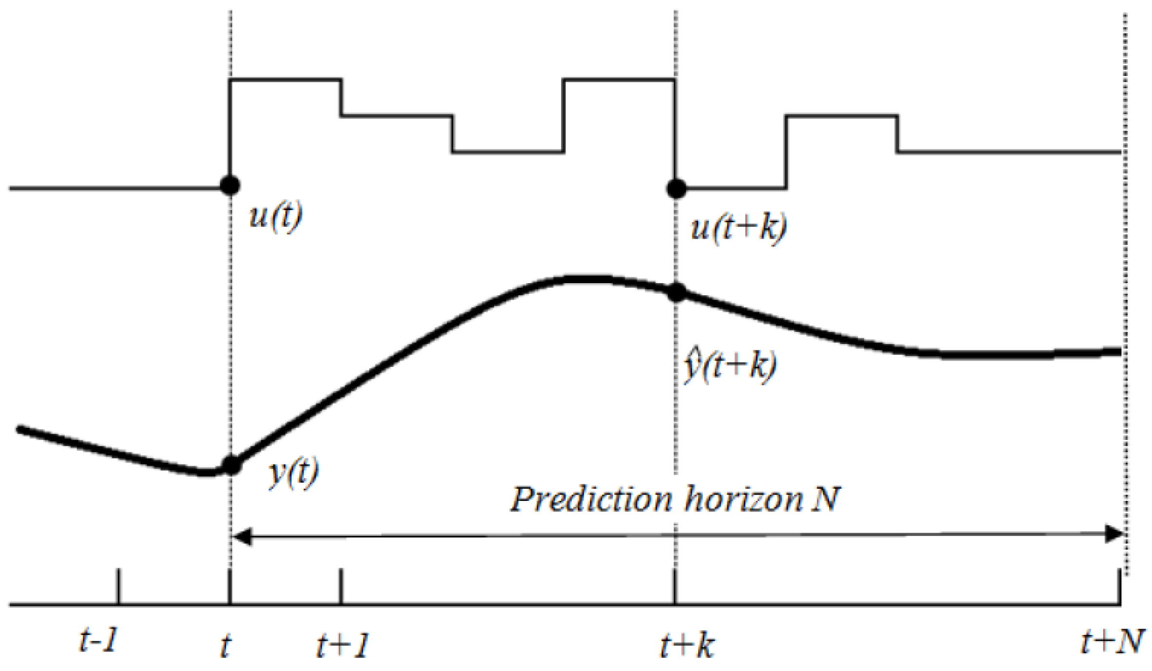
Figure 5.
Flowchart of MPC’s steps.

Figure 6.
Standard flowchart of PSO.

Figure 7.
Frequency deviation in Area 1 for the first case.

Figure 8.
Frequency deviation in Area 2 for the first case.
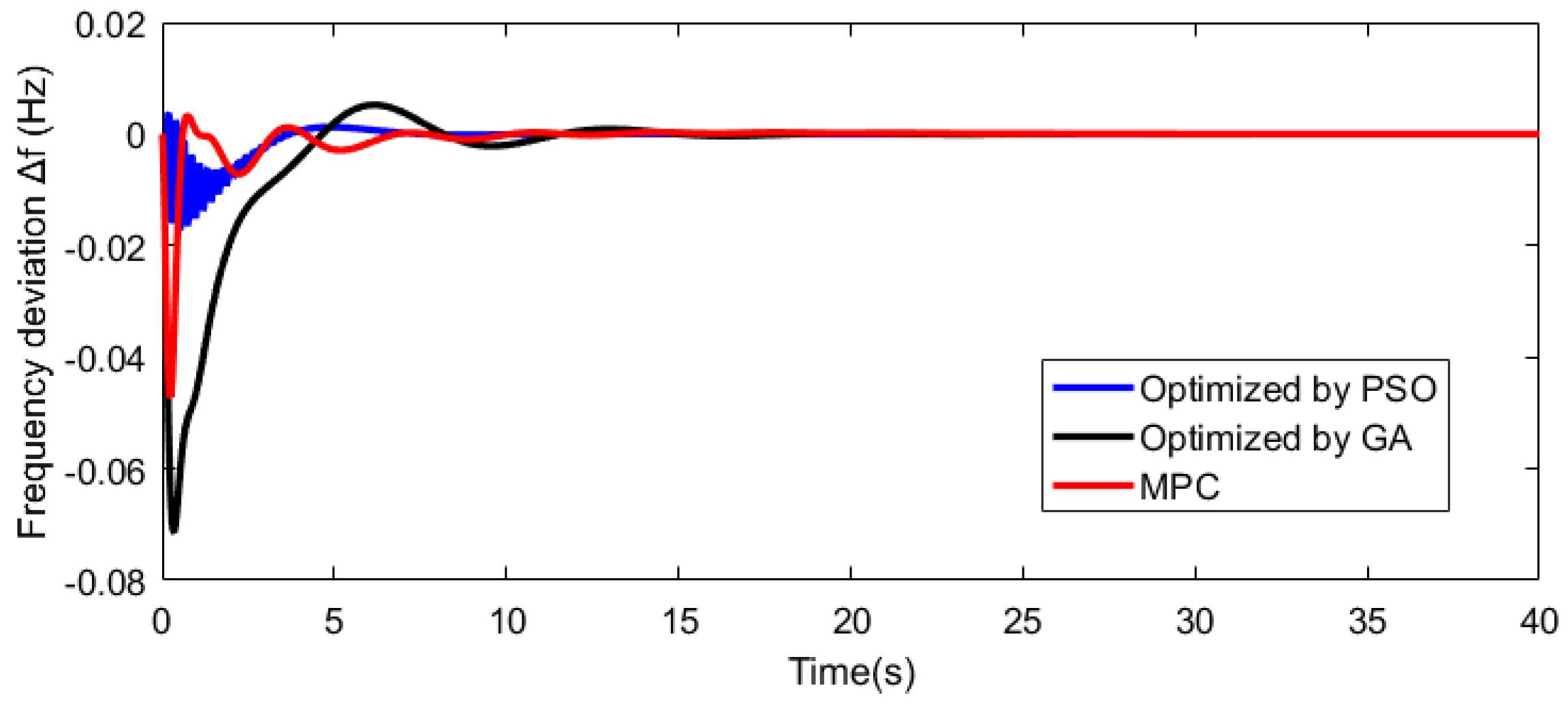
Figure 9.
Tie-line power deviation for the first case.
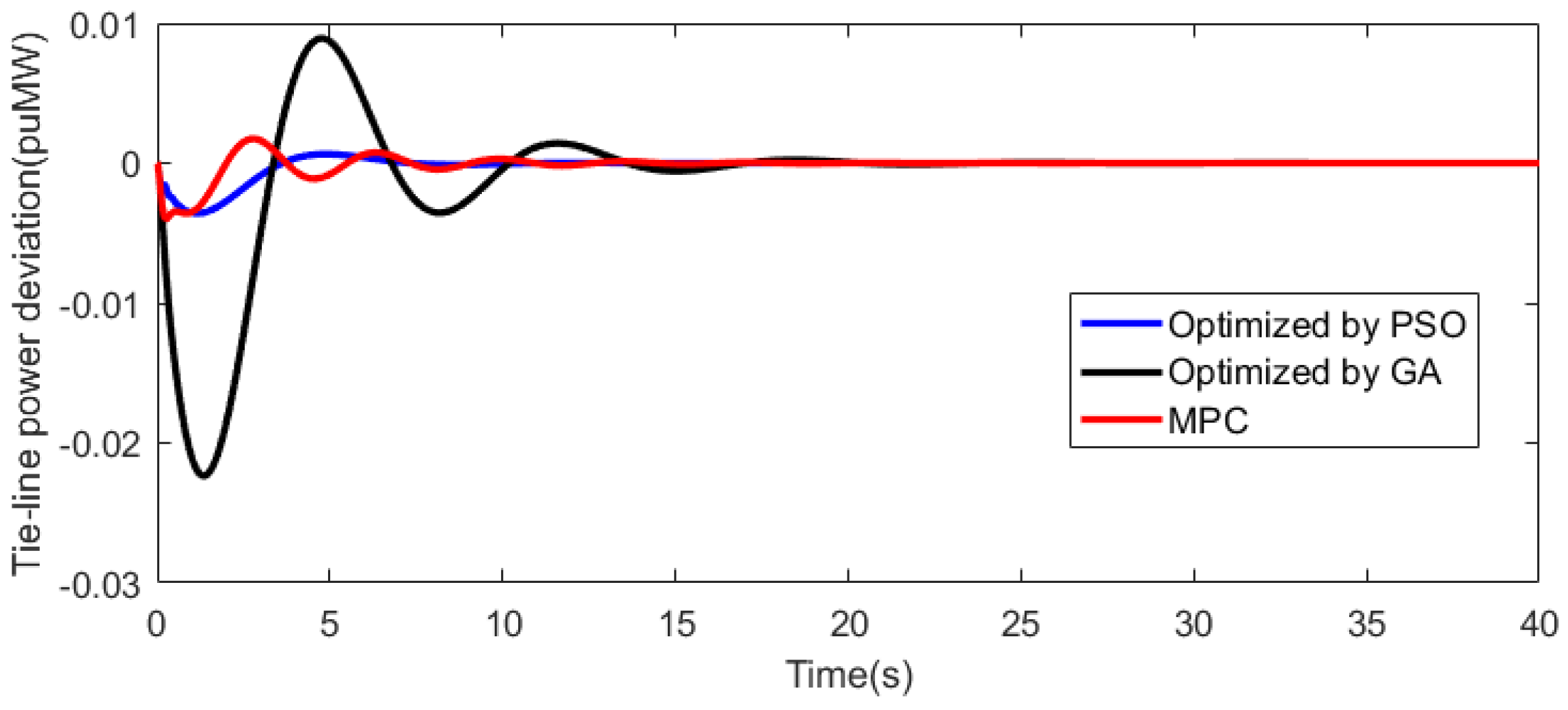
Figure 10.
Frequency deviation in Area 1 for the second case.

Figure 11.
Frequency deviation in Area 2 for the second case.

Figure 12.
Tie-line power deviation for the second case.
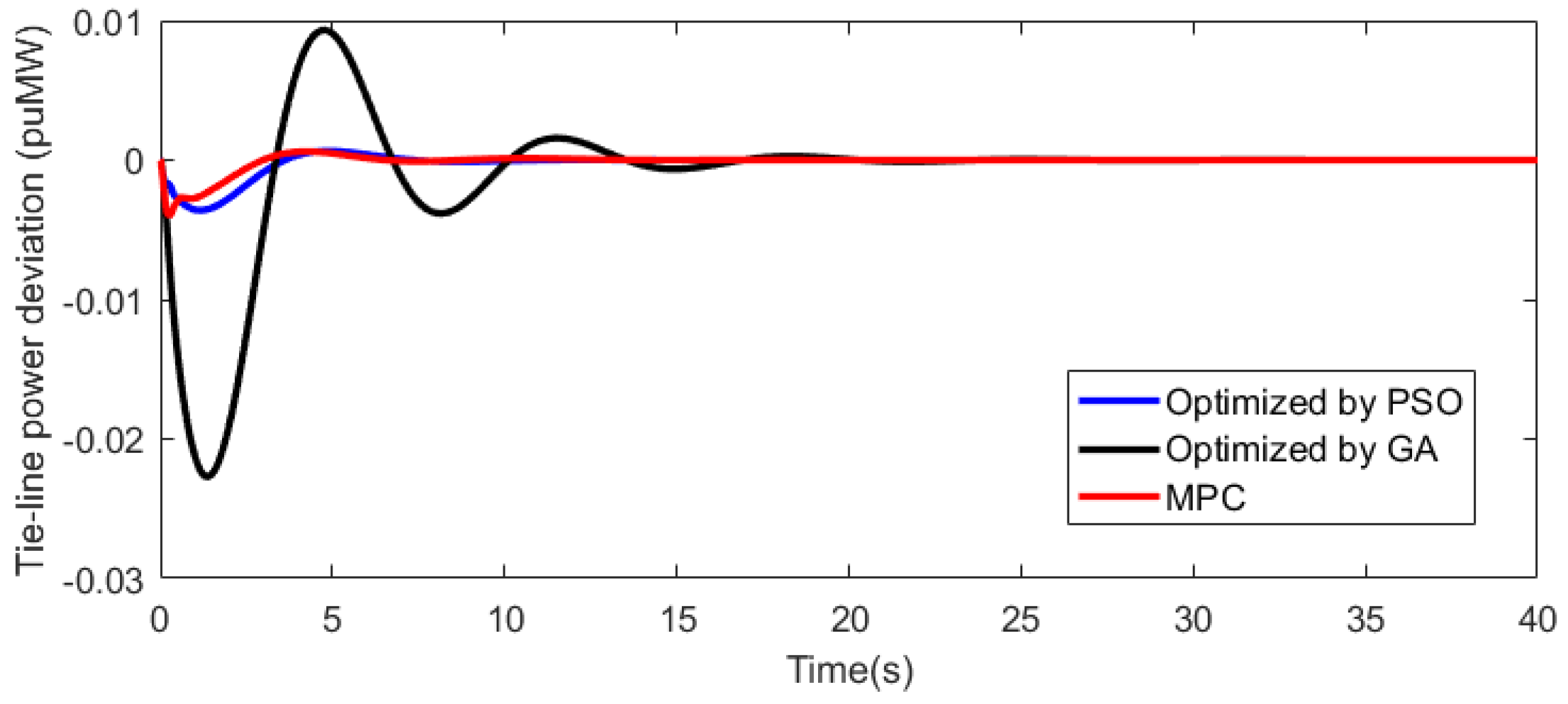
Figure 13.
Frequency deviation in Area 1 for the third case.

Figure 14.
Frequency deviation in Area 2 for the third case.

Figure 15.
Tie-line power deviation for the third case.

Figure 16.
Frequency deviation in Area 1 for the fourth case.

Figure 17.
Frequency deviation in Area 2 for the fourth case.

Figure 18.
Tie-line power deviation for the fourth case.
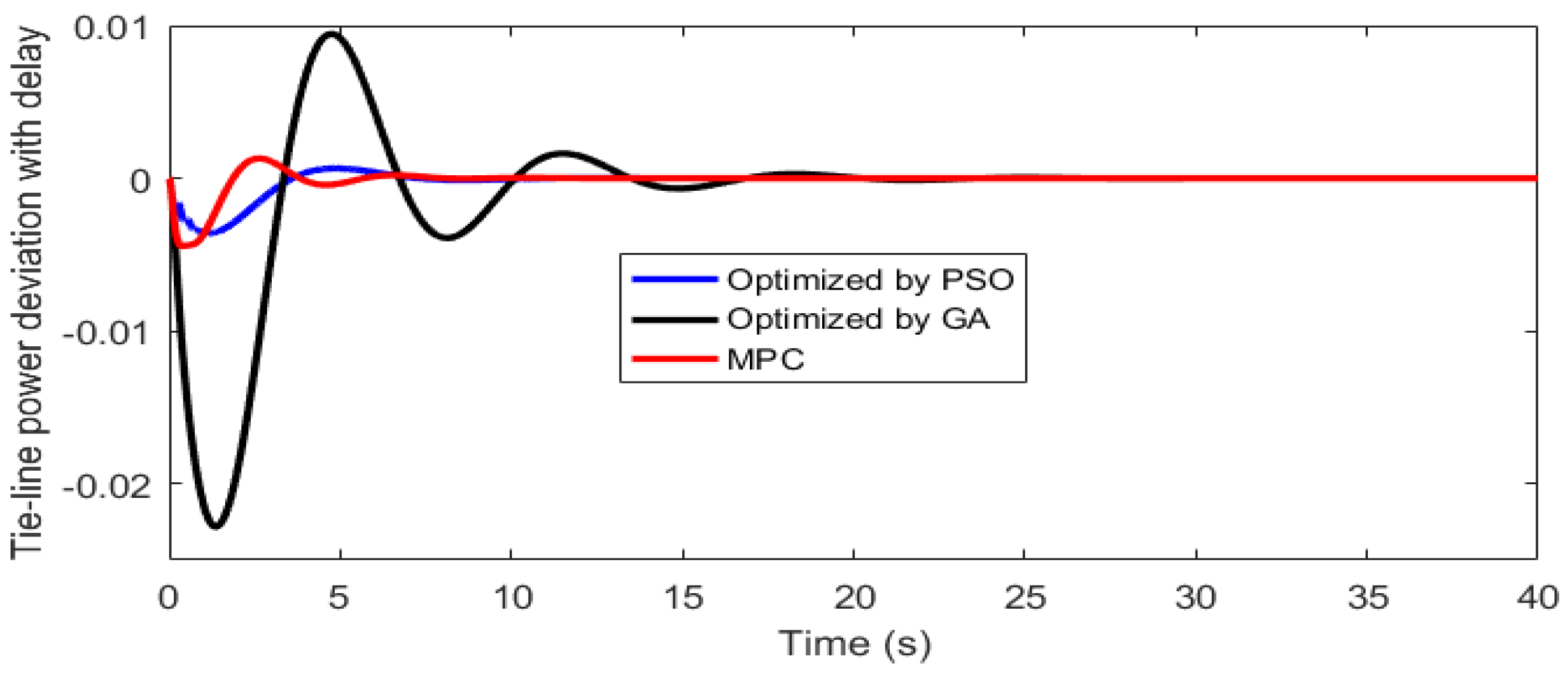
Figure 19.
Pole-zero map of MPC-based frequency control loops.

Figure 20.
Pole-zero map of GA-based frequency control loops.
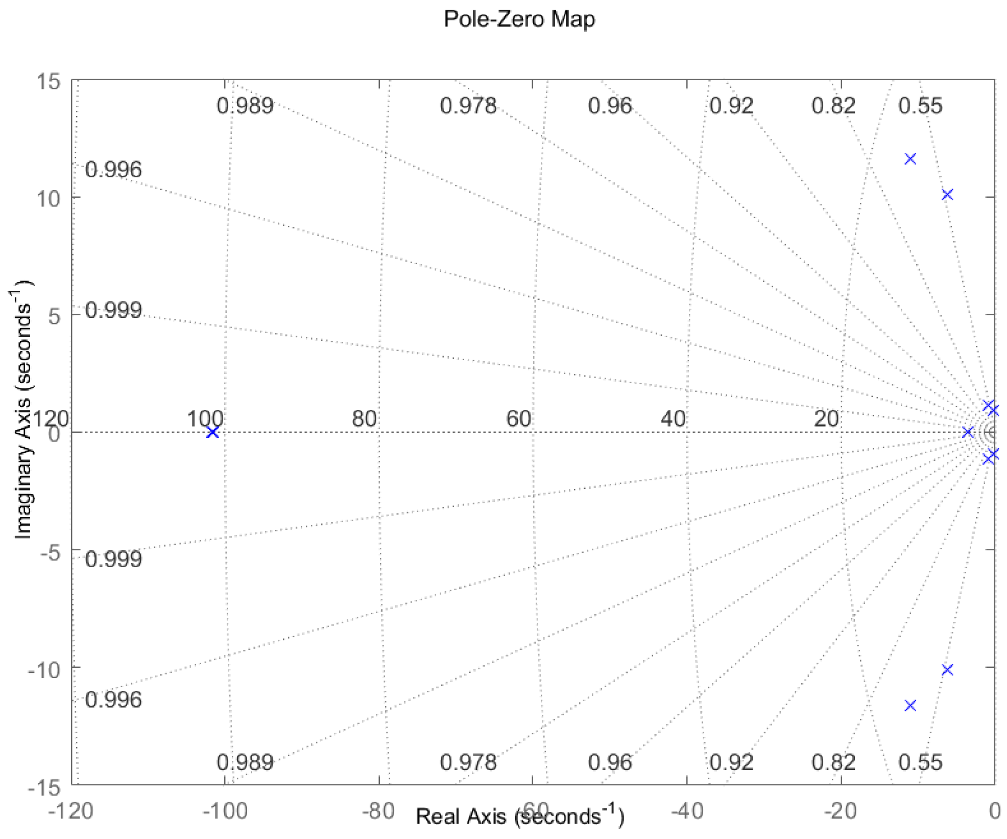
Figure 21.
Pole-zero map of PSO-based frequency control loops.


Table 1.
Parameters used.
| Parameter | Value | |
|---|---|---|
| Synchronizing coefficients for tie lines for the two-area system | (pu MW) | 0.545 |
| Power system time constants in Areas 1 and 2 | = (s) | 20 |
| Turbine time constants in Areas 1 and 2 | = (s) | 0.3 |
| Governor time constants in Areas 1 and 2 | = (s) | 0.008 |
| Power system constants in Areas 1 and 2 | = (Hz/puMW) | 120; 84 |
| Regulations of governors in Areas 1 and 2 | = (Hz/pu MW) | 2.4 |
| Tie line frequency bias in Areas 1 and 2 | = (pu MW/Hz) | 0.425 |
Table 2.
Optimized PID controller gain.
| PID Parameters | |||
|---|---|---|---|
| GA optimized PID | 1.93 | 3.00 | 1.20 |
| PSO optimized PID | 15.0 | 15.0 | 14.1 |
Table 3.
Dynamic response comparison in terms of peak overshoot.
| GA base | 0.019 | 0.006 | 0.007 |
| PSO base | 0.009 | 0.005 | 0.001 |
| MPC base | 0.004 | 0.002 | 0.001 |
| GA with variation , | 0.019 | 0.004 | 0.007 |
| PSO with variation , | 0.006 | 0.001 | 0.001 |
| MPC with variation , | 0.012 | 0.013 | 0.001 |
| GA with variation | 0.020 | 0.005 | 0.007 |
| PSO with variation | 0.006 | 0.002 | 0.002 |
| MPC with variation | 0.012 | 0.013 | 0.002 |
| GA with time delay | 0.019 | 0.010 | 0.009 |
| PSO with time delay | 0.018 | 0.011 | 0.001 |
| MPC with time delay | 0.018 | 0.010 | 0.001 |
Table 4.
Dynamic response comparison in terms of peak undershoot.
| GA base | 0.11 | 0.050 | 0.022 |
| PSO base | 0.03 | 0.015 | 0.003 |
| MPC base | 0.06 | 0.045 | 0.004 |
| GA with variation , | 0.130 | 0.062 | 0.022 |
| PSO with variation , | 0.030 | 0.010 | 0.004 |
| MPC with variation , | 0.070 | 0.040 | 0.004 |
| GA with variation | 0.130 | 0.061 | 0.023 |
| PSO with variation | 0.030 | 0.011 | 0.005 |
| MPC with variation | 0.070 | 0.041 | 0.005 |
| GA with time delay | 0.110 | 0.067 | 0.026 |
| PSO with time delay | 0.030 | 0.025 | 0.005 |
| MPC with time delay | 0.080 | 0.030 | 0.005 |
Table 5.
Dynamic response comparison in terms of settling Time.
| GA base | 7.00 | 8.00 | 10.00 |
| PSO base | 4.00 | 4.00 | 5.00 |
| MPC base | 3.00 | 4.00 | 5.00 |
| GA with variation , | 8.00 | 9.00 | 11.00 |
| PSO with variation , | 3.00 | 4.00 | 4.00 |
| MPC with variation , | 3.00 | 4.00 | 4.00 |
| GA with variation | 8.00 | 9.00 | 12.00 |
| PSO with variation | 3.00 | 4.00 | 6.00 |
| MPC with variation | 3.00 | 5.00 | 4.00 |
| GA with time delay | 8.00 | 8.00 | 12.00 |
| PSO with time delay | 8.00 | 8.00 | 4.00 |
| MPC with time delay | 3.00 | 3.00 | 4.00 |
Table 6.
MPC, PSO and GA based frequency control loops poles.
| Genetic Algorithm | Particle Swarm Optimization | Model Predictive Controller |
|---|---|---|
| −101.61 + | − + | − + |
| −101.46 + | − + | − + |
| −11.10 + | − + | − − |
| −11.10 − | − − | − + |
| −6.22 + | − + | − + |
| −6.22 − | − − | − − |
| −0.3000 + | −27.00 + | |
| −0.3000 − | −0.46 + | |
| −0.99 + | −0.46 − | |
| −0.99 − | −0.55 + | |
| −3.49 + | −0.55 − |
© 2018 by the authors. Licensee MDPI, Basel, Switzerland. This article is an open access article distributed under the terms and conditions of the Creative Commons Attribution (CC BY) license (http://creativecommons.org/licenses/by/4.0/).
Share and Cite
MDPI and ACS Style
Charles, K.; Urasaki, N.; Senjyu, T.; Elsayed Lotfy, M.; Liu, L. Robust Load Frequency Control Schemes in Power System Using Optimized PID and Model Predictive Controllers. Energies 2018, 11, 3070. https://doi.org/10.3390/en11113070
AMA Style
Charles K, Urasaki N, Senjyu T, Elsayed Lotfy M, Liu L. Robust Load Frequency Control Schemes in Power System Using Optimized PID and Model Predictive Controllers. Energies. 2018; 11(11):3070. https://doi.org/10.3390/en11113070
Chicago/Turabian StyleCharles, Komboigo, Naomitsu Urasaki, Tomonobu Senjyu, Mohammed Elsayed Lotfy, and Lei Liu. 2018. "Robust Load Frequency Control Schemes in Power System Using Optimized PID and Model Predictive Controllers" Energies 11, no. 11: 3070. https://doi.org/10.3390/en11113070
Note that from the first issue of 2016, this journal uses article numbers instead of page numbers. See further details here.