Control of a DC-DC Buck Converter through Contraction Techniques

Abstract

Reliable and robust control of power converters is a key issue in the performance of numerous technological devices. In this paper we show a design technique for the control of a DC-DC buck converter with a switching technique that guarantees both good performance and global stability. We show that making use of the contraction theorem in the Jordan canonical form of the buck converter, it is possible to find a switching surface that guarantees stability but it is incapable of rejecting load perturbations. To overcome this, we expand the system to include the dynamics of the voltage error and we demonstrate that the same design procedure is not only able to stabilize the system to the desired operation point but also to reject load, input voltage, and reference voltage perturbations.

1. Introduction

Many industrial and residential applications use voltage regulation with DC-DC power converters; such applications include fuel cells [1], photovoltaic sources [2,3], control of DC motors [4], lighting appliances [5], computer power supplies [6], and many others. Power converters transform a non regulated voltage/current source (DC or AC) into a regulated voltage/current output, which can be either larger or smaller than the non regulated input. Usually, the underlying structures in these devices are the so-called buck (step-down), boost (step-up), buck-boost (step down-step up), flyback, Ćuk, to mention few, depending on the type of application [7,8]. DC-DC power converters show both fast speed and capability of managing high power if needed [9]. More than 90% of the total amount of power supply in the world is processed through power converters [10]. For this reason, a precise control of these converters is a critical factor and therefore a vast amount of literature has been devoted to their control. For instance, PID-based schemes [11], Fuzzy PID control [12], robust controllers [13], predictive control [14], sliding mode control [15], and a controller based on a modified pulse-adjustment of the PWM [16], just to mention few.

The DC-DC buck power converter supplies a lower voltage than the input voltage and is one of the most widely studied power converters: Some recent applications include battery chargers [17], hybrid electric vehicles [18], quadropter’s control [19], among others. The underlying topology of the buck converter is non-smooth, meaning that it switches back and forth according to a control signal, between an ON and OFF state, to guarantee a required output voltage. Some examples of control techniques applied to the buck converter include zero voltage control technique [20], fractional derivative control [21], controller based on active ramp tracking [22], and fuzzy PID controllers [23].

Even though the effectiveness of these control actions is out of doubt, usually the design of such controllers are based either on the averaged version of the system which effectively disregards the non-smoothness; or via linearization. This is because the effect of the nonlinearity is not always entirely understood and therefore the system can only be analyzed in the vicinity of the operation point (see [24] for a review on stability methods). This may result in undesired effects such as destabilization when the system is far from the operation point and limits the range of operation in which the DC-DC converter can work. This is because linearizing the system can only assure local stability, and the region of attraction is usually unknown.

Recently, a novel method to design an asymptotically globally stable controller for switched systems has been introduced in the literature [25,26] following the ideas of contraction theory, also used in [27]. Inspired by these papers, where some illustrative cases were developed in a few academic examples with limited application into the physical realm, the aim of this paper is to use the novel concepts of contraction theory on switched systems to design a switched controller that guarantees asymptotic global stability on the buck DC-DC power converter. With this purpose, the paper is organized as follows: In Section 2 we present some preliminary concepts needed for the development of the paper, specifically on linear transformations, matrix measure, Filippov systems, and contraction theory. After, in Section 3, the buck power converter is presented as well as its principle of operation. In Section 4, a controller based on contraction theory is designed and tested for the buck power converter. As the system is not robust, in Section 5 we develop a modified control action that uses the principles of integral control which shows robustness preserving global stability. We conclude this paper with some remarks and future perspectives.

2. Mathematical Methods

In this section we present some standard theory on linear systems (see [28]), matrix measures [29,30,31] and contraction theory applied to stability of switched systems [25,26] Most of the material can be found in the cited documents and references therein.

2.1. Linear Transformations

Let us consider the piece-wise linear system (PWLS) given by

$$\dot{\mathbf{x}}=A\mathbf{x}+Bu,$$

(1)

where $u\in \{u_1,u_2\}$ and it commutes between booth values depending on the value of the switching surface $h\left(\mathbf{x}\right)$ = 0. A is a Hurwitz matrix, the pair $(A,B)$ is controllable and all eigenvalues are distinct but not necessarily real. Then, there exists a real matrix P which transforms the original system into a canonical form, so called the Jordan form, in the following way:

$$A_J=P^{-1}AP{B}_J=P^{-1}B.$$

(2)

The transformation matrix can be constructed as follows: For each real eigenvalue, its corresponding eigenvector is computed and assigned to one column of the matrix P. For every pair of complex eigenvalues their corresponding complex eigenvectors are computed but only one of them is used to construct two column vectors of the matrix P. The first one is composed by the real parts of the complex eignevector, while the other one is composed by the imaginary parts of the same eigenvector. For example, in a system with one real eigenvector ${\mathbf{v}}_1$ and two complex conjugate ${\mathbf{v}}_2$ and ${\widehat{\mathbf{v}}}_2$ the matrix P takes the form

$$P=\left[{\mathbf{v}}_1\mathrm{Re}\left({\mathbf{v}}_2\right)\mathrm{Im}\left({\mathbf{v}}_2\right)\right].$$

(3)

Using this transformation matrix we obtain that every real eigenvalue (${\lambda }_j={\eta }_j$) produces a column in the matrix $A_J$ with the eigenvalue in the corresponding diagonal element with other elements equal to zero. Every complex pair of eigenvalues (${\lambda }_{k,k+1}={\alpha }_k\pm {\beta }_k$) instead, generates a $2\times 2$ block in the Jordan matrix such that the diagonal part corresponds to the real part of the eigenvalues and the other positions correspond to the positive and negative imaginay part: Other elements are zero. A general example of this Jordan form is:

$$\begin{array}{c}{A}_J=\left[\begin{array}{ccccccc}{\eta }_1& 0& 0& 0& 0& 0& \cdots \\ 0& \ddots & 0& 0& 0& 0& \cdots \\ 0& \cdots & {\alpha }_k& -{\beta }_k& 0& 0& \cdots \\ 0& \cdots & {\beta }_k& {\alpha }_k& 0& 0& \cdots \\ 0& \cdots & 0& 0& {\alpha }_{k+2}& -{\beta }_{k+2}& \cdots \\ 0& \cdots & 0& 0& {\beta }_{k+2}& {\alpha }_{k+2}& \cdots \\ ⋮& ⋮& ⋮& ⋮& ⋮& ⋮& \ddots \end{array}\right].\end{array}$$

(4)

2.2. Matrix Measure

The norm-2 induced measure of a matrix A is defined as:

$${\mu }_2\left(A\right)={\lambda }_{max}[A^{\prime }+A]/2,$$

(5)

where ${\lambda }_{max}[·]$ is the largest eigenvalue and $A^{\prime }$ is the transpose of A. It is possible to verify that, if the matrix A in (1) is Hurwitz, then ${\mu }_2\left(A_J\right)$ is always negative. This is an important issue in the stability analysis performed in this paper.

2.3. Contraction Analysis for Filippov Systems

Another way to define the system (1) is as a bimodal Filippov system

$$\dot{\mathbf{x}}=\left\{\begin{array}{cc}{F}^{+}\left(\mathbf{x}\right)\hfill & \mathrm{if}\mathbf{x}\in S^{+}\hfill \\ F^{-}\left(\mathbf{x}\right)\hfill & \mathrm{if}\mathbf{x}\in S^{-}.\hfill \end{array}\right.$$

(6)

where

$$F^{+}\left(\mathbf{x}\right)=A\mathbf{x}+B{u}_1\mathrm{and}{F}^{-}\left(\mathbf{x}\right)=A\mathbf{x}+B{u}_2$$

being

$$S^{+}=\{\mathbf{x}\in \mathcal{U}:h\left(\mathbf{x}\right)>0\}\mathrm{and}{S}^{-}=\{\mathbf{x}\in \mathcal{U}:h\left(\mathbf{x}\right)<0\}.$$

Here, $h:\mathcal{U}\to R$ is a smooth function called switching function and the surface $\mathsf{\Sigma }$ defined as

$$\mathsf{\Sigma }=\{\mathbf{x}\in \mathcal{U}:h(\mathbf{x})=0\}$$

(7)

is called the switching surface.

According to [25,26], the bimodal Filippov system (6) is incrementally exponentially stable in a so-called K-reachable set $\mathcal{C}\subseteq \mathcal{U}$ with convergence rate $r=min\{r_1,r_2\}$, if there exists some norm in $\mathcal{C}$ with associated measure $\mu$ such that for some positive constants $r_1,r_2$

$$\begin{array}{c}\hfill \mu \left({\displaystyle \frac{\partial F^{+}\left(\mathbf{x}\right)}{\partial \mathbf{x}}}\right)\le -r_1\forall \mathbf{x}\in \overline{S^{+}},\\ \hfill \mu \left({\displaystyle \frac{\partial F^{-}\left(\mathbf{x}\right)}{\partial \mathbf{x}}}\right)\le -r_2\forall \mathbf{x}\in \overline{S^{-}},\end{array}$$

(8)

and

$$\mu ((F^{+}\left(\mathbf{x}\right)-F^{-}\left(\mathbf{x}\right))·\nabla h\left(\mathbf{x}\right))=0\forall \mathbf{x}\in \mathsf{\Sigma },$$

(9)

where $\overline{S^{+}}$ and $\overline{S^{-}}$ represent the closures of the sets $S^{+}$ and $S^{-}$ respectively.

If system (6) is incrementally exponentially stable then there exist constants $k\ge 1$ and $\lambda >0$ such that

$$|\mathbf{x}\left(t\right)-\mathbf{y}\left(t\right)|\le k{e}^{-\lambda (t-t_0)}|\mathbf{x}\left(0\right)-\mathbf{y}\left(0\right)|\forall t\ge t_0\forall \mathbf{x}\left(0\right),\mathbf{y}\left(0\right)\in \mathcal{C}$$

where $\mathbf{x}\left(t\right)$ and $\mathbf{y}\left(t\right)$ are solutions of the system. Thus we can establish global stability properties for system (1). Making use of the previous concepts, we will design an hybrid control for a buck power converter that guarantees not only global stability, but is also robust to different disturbances.

3. The Buck Power Converter

The scheme of a buck power converter is depicted in Figure 1. The equations describing this dynamical system in Continuous Conduction Mode CCM (see [10,32,33]) are

$$\left(\begin{array}{c}\dot{v}\\ \dot{i}\end{array}\right)=\left(\begin{array}{cc}-\frac{1}{RC}& \frac{1}{C}\\ -\frac{1}{L}& 0\end{array}\right)\left(\begin{array}{c}v\\ i\end{array}\right)+\left(\begin{array}{c}0\\ \frac{E}{L}\end{array}\right)u$$

(10)

where R is the load resistance, C is the capacitor’s capacitance, L is the coil’s inductance, and E is the voltage provided by the power source. The state variable v corresponds to the voltage across the capacitor and i quantifies the current flowing through the inductor. The control signal u takes values in the discrete set $\{0,1\}$. When $u=0$ the switch is opened and the power source (input voltage) does not feed the system. In this case, the load is being fed by the capacitor and the inductor. For simplicity we will perform a first transformation which maps the original system (10) into a dimensionless framework by means of the following similarity transformation $x=M^{-1}{\left(vi\right)}^{\prime }$, where

$$M=\left(\begin{array}{cc}E& 0\\ 0& \frac{E}{\sqrt{L/C}}\end{array}\right)$$

(11)

Also we perform a normalization of the time as $\tau =t/\sqrt{LC}$, such that a new and unique parameter $\gamma =\frac{1}{R}\sqrt{\frac{L}{C}}$ holds the information of the parameters in the system. Therefore we can rewrite the equations as:

$$\left(\begin{array}{c}{\dot{x}}_1\\ {\dot{x}}_2\end{array}\right)=\left(\begin{array}{cc}-\gamma & 1\\ -1& 0\end{array}\right)\left(\begin{array}{c}{x}_1\\ x_2\end{array}\right)+\left(\begin{array}{c}0\\ 1\end{array}\right)u$$

(12)

or in a compact form as $\dot{\mathbf{x}}=A\mathbf{x}+Bu$.

With the aim of designing the controller, it is necessary to transform the system to the Jordan normal form. As the pair $(A,B)$ is controllable, then as outlined in Section 2.1, there exists a transformation matrix P given by

$$P=\left(\begin{array}{cc}\gamma /2& \rho \\ 1& 0\end{array}\right)$$

(13)

which transforms the system into:

$$\left(\begin{array}{c}{\dot{z}}_1\\ {\dot{z}}_2\end{array}\right)=\left(\begin{array}{cc}-\gamma /2& -\rho \\ \rho & -\gamma /2\end{array}\right)\left(\begin{array}{c}{z}_1\hfill \\ z_2\hfill \end{array}\right)+\left(\begin{array}{c}1\\ -\gamma /\left(2\rho \right)\end{array}\right)u$$

(14)

where $\mathbf{z}=P^{-1}\mathbf{x}$ and we have used $\rho :=\rho \left(\gamma \right)=\sqrt{4-{\gamma }^2}/2$. These equations are noted in a compact form as $\dot{\mathbf{z}}=A_J\mathbf{z}+B_{J}u$.

4. Application to 2D-Case

4.1. Controller Design

Using the contraction theorem outlined in Section 2.3, we can establish that the converter operating with the switched signal control u will be stable if the following two conditions are satisfied:

$$\begin{array}{c}a){\mu }_2\left(A_J\right)<-r_1,\forall \mathbf{z}\hfill \\ b){\mu }_2(B_J·\nabla h\left(\mathbf{z}\right))=0,\forall \mathbf{z}\in h\left(\mathbf{z}\right)=0.\hfill \end{array}$$

(15)

One can easily show that ${\mu }_2\left(A_J\right)=-\gamma /2$, hence condition (a) is always met as $\gamma$ is always positive. Then, considering $h\left(\mathbf{z}\right)$ as a linear function of the states $h\left(\mathbf{z}\right)=\left(h_1{h}_2\right)·{\left(z_1{z}_2\right)}^{\prime }$, the condition (b) can be written as:

$${\mu }_2\left(\left(\begin{array}{c}1\\ -\gamma /\left(2\rho \right)\end{array}\right)·\left(h_1{h}_2\right)\right)=0.$$

(16)

It is possible to demonstrate (see Appendix A) that the following choice of $h\left(\mathbf{z}\right)$:

$$\begin{array}{ccc}\hfill h\left(\mathbf{z}\right)& =& h_1{z}_1+\frac{B_J\left(2\right)}{B_J\left(1\right)}{h}_1{z}_2=\left(h_1-h_1\gamma /\left(2\rho \right)\right)·{\left(z_1{z}_2\right)}^{\prime }:=h_z·\mathbf{z},\hfill \end{array}$$

(17)

where $B_J\left(i\right)$ is the $i-th$ row element in $B_J$, fulfills condition (16) if the pairs $\{B_J\left(i\right),h\left(i\right)\}$ have opposite signs. Then, according to the signs of $B_J\left(i\right)$, it is necessary to choose $h_1<0$ and $h_2>0$. In this way, the matrix from which the maximum eigenvalue needs to be calculated according to Equation (5), has one null eigenvalue and the other one can be computed as ${\lambda }_2=h_1/{\rho }^2$, which is smaller than zero. Since the switching surface has been calculated in the canonical space, this result needs to be transformed back into the dimensionless state variables through $\mathbf{x}=P\mathbf{z}$. The switching manifold is then obtained as $h\left(\mathbf{x}\right)=h_z·P^{-1}·\mathbf{x}$, or equivalently:

$$\begin{array}{ccc}h\left(\mathbf{x}\right)\hfill & =\hfill & \left(h_1{h}_1{(1+(\gamma /\left(2\rho \right))}^2\right)·{\left(x_1{x}_2\right)}^{\prime }:=h_x·\mathbf{x}\hfill \end{array}$$

(18)

Of course, the term $h_x$ correspond the vector in the normal direction of the switching surface. With the aim of simplifying the calculations we normalize such vector such that $|h_x|=1$. Moreover, we need to subtract the reference values to the states to ensure the regulation to the operation point.

$$\begin{array}{ccc}h\left(\mathbf{x}\right)\hfill & =\hfill & \left(-\frac{\gamma }{\sqrt{4+{\gamma }^2}}\frac{2}{\sqrt{4+{\gamma }^2}}\right)·{(x_1-{\overline{x}}_{1ref}{x}_2-{\overline{x}}_{2ref})}^{\prime }=0.\hfill \end{array}$$

(19)

Finally, we can define the switching manifold in terms of the original state variables $\left(x_1{x}_2\right)=M^{-1}{\left(vi\right)}^{\prime }$ leading to:

$$\begin{array}{ccc}h(v,i)\hfill & =\hfill & \left(-\frac{\gamma }{E\sqrt{4+{\gamma }^2}}\frac{2\sqrt{L/C}}{E\sqrt{4+{\gamma }^2}}\right)·{(v-{\overline{v}}_{ref}i-{\overline{i}}_{ref})}^{\prime }=0.\hfill \end{array}$$

(20)

It is worth noticing that neither $h_1$ nor $h_2$ appear in the calculations. On the one hand $h_2$ is parametrized via $h_1$ (see Appendix A), on the other hand $h_1$ disappear via the normalization, reducing effectively two degrees of freedom. Also, for the sake of simplifying the calculations we have considered a switching function with zero offset. Introducing the offset in this function, which amounts to perform a translation of the switching surface, does not change any of the stability criteria that we are presenting here and can indeed be employed as a further degree of freedom.

4.2. Simulation Results

The design methodology described so far is independent of the parameters. However, in order to show the numerical behavior in a realistic set up we will use the following set of parameters for numerical computations: $L=$2 mH, $C=40\mathsf{\mu }$F, $E=40$ V, and ${\overline{v}}_{ref}=32$ V. This range of input/output operation can be found, for instance, in solar panel arrays feeding a battery charger through a buck converter. In our particular numerical example we will assume a load $R=20\mathsf{\Omega }$. The desired current reference can be assumed to be ${\overline{i}}_{ref}={\overline{v}}_{ref}/R=1.6$ A. With this, $\gamma \approx 0.35$ and $\rho \approx 0.98$. Also, as electronic devices cannot switch with infinite speed, it is necessary to implement a hysteresis band for simulating the change in the position of the MOSFET. We have designed this band in such a way that the switching time is close to 175 $\mathsf{\mu }$s. The size of the hysteresis band is an important issue because its width also determines the size of the chattering in the voltage variable. Under these assumptions, Equation (20) takes the following values:

$$\begin{array}{c}h(v,i)=\left(-4.4\times {10}^{-3}0.1741\right)·{(v-{\overline{v}}_{ref}i-{\overline{i}}_{ref})}^{\prime }\pm 0.02\end{array}$$

(21)

In Figure 2 we show the performance of the designed control. In particular, in Figure 2a the time trace of the voltage v is depicted in response to a drastic change in the reference output voltage ${\overline{v}}_{ref}$. During the first 30 ms, where the system is subject to ${\overline{v}}_{ref}=32$ V (top dashed line), the output voltage reaches the steady state close to $5.7$ ms, with no overshoot and the maximum error in steady state is lower than $0.6\%$ (see inset). After 30 ms, the reference voltage is changed to ${\overline{v}}_{ref}=16$ V (bottom dashed line) and the system is able to track the change and stabilize to the new value of output voltage. In Figure 2b,c we plot the orbit in the $(v,i)$ space during the steady state for the two references used in panel A) of the same figure. From this, one can observe that indeed the equilibrium value $({\overline{v}}_{ref},{\overline{i}}_{ref})$ is reached through the continuous rippling of the orbit around the equilibrium point (red symbol).

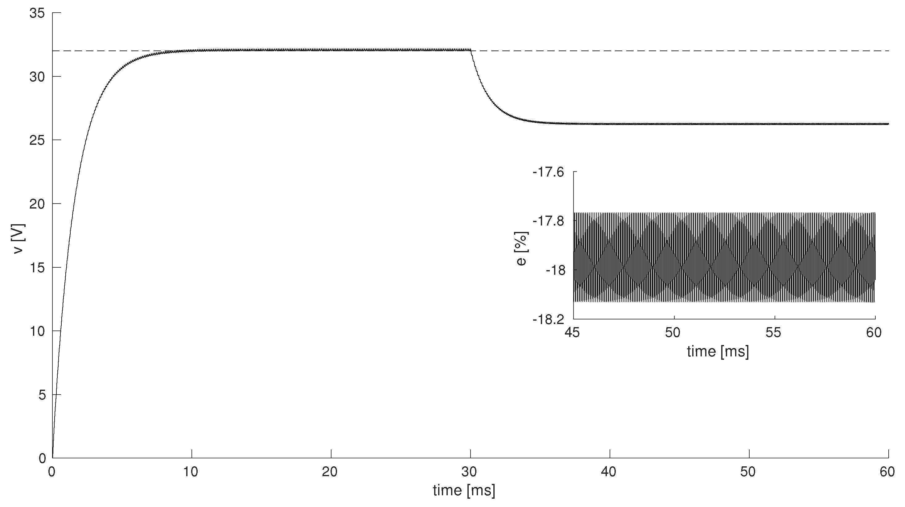
We also tested the robustness of the control to changes in the load. In Figure 3 is depicted the time trace of the voltage in this scenario. Following a similar procedure as in Figure 2, after 30 ms, a change in the resistance from $R=20\mathsf{\Omega }$ to $R=15\mathsf{\Omega }$ (10% difference) is applied. From this figure it is possible to see that the system drifts away from the reference output ${\overline{v}}_{ref}=32$ V (dashed line), producing a steady state error of around 18% (see inset).

So far, the controller designed with contraction theory has been successful to operate in a desired way and reject disturbances in the output voltage. However, when a disturbance in the load is presented (a common situation in power converters) the system loses the ability to follow the desired output voltage, indicating that the controller is not robust. To solve this problem, we extend the proposed controller based on the idea of an integral control action.

5. Application to 3D-Case

5.1. Controller Design Based on a Modified Integral Control Action

In control theory it is known that perturbations are better rejected by a PI controller; however, in this case, adding a PI controller implies to add a pole in the origin of the system which prevents us from applying contraction theorem. Then, with the aim of enhancing the robustness of the controlled system, we will modify the control action in such a way that it introduces the dynamics of the error. To do so we introduce a new state variable $x_3$ in the dimensionless system in the following way: ${\dot{x}}_3=e-\delta x_3$, with $e={\overline{x}}_{1ref}-x_1$ defined as the output error and $\delta$ as the time constant of $x_3$. As $x_1=v/E$, then ${\overline{x}}_{1ref}={\overline{v}}_{ref}/E$. Under these assumptions, the system takes the following form:

$$\begin{array}{c}\hfill l\left(\begin{array}{c}{\dot{x}}_1\\ {\dot{x}}_2\\ {\dot{x}}_3\end{array}\right)=\left(\begin{array}{ccc}-\gamma & 1& 0\\ -1& 0& 0\\ -1& 0& -\delta \end{array}\right)\left(\begin{array}{c}{x}_1\\ x_2\\ x_3\end{array}\right)+\left(\begin{array}{c}0\\ 1\\ 0\end{array}\right)u+\left(\begin{array}{c}0\\ 0\\ 1\end{array}\right){\overline{x}}_{1ref}\end{array}$$

(22)

with

$$u=\left\{\begin{array}{cc}1\hfill & \mathrm{if}h\left(\mathbf{x}\right)\le 0\hfill \\ 0\hfill & \mathrm{otherwise}.\hfill \end{array}\right.$$

(23)

or in compact form $\dot{\mathbf{x}}=A\mathbf{x}+Bu+Q{\overline{x}}_{1ref}$. The aim of the term $-\delta$ appearing in position $\{3,3\}$ in the matrix A is to stabilize the system allowing us to apply the contraction theorem. In this way, the value of $\delta$ must be very small to avoid high steady state error. As the pair $(A,B)$ is controllable we then proceed to apply the general theory with a new consideration: In the construction of the matrix P we will take into account the norm of the eigenvectors ${\mathbf{v}}_i$, which will allow us to gain more degrees of freedom in the system to tune the controller. Indeed this is not an issue when obtaining the canonical form $A_J$ as the operation $P^{-1}AP$ cancels out any norm that may have been considered. However, the transformed matrix $B_J$, which is critical for the stability conditions Equation (15), may depend on the chosen modules of the eigenvectors. To take this into account, we need to include in Equation (3) the magnitude of the eigenvectors via the scaling factors $c_1$ and $c_2$ as follows:

$$P=\left[c_1{\mathbf{v}}_1{c}_2\mathrm{Re}\left({\mathbf{v}}_2\right)c_2\mathrm{Im}\left({\mathbf{v}}_2\right)\right].$$

(24)

The general form of the transformation matrix can then be written as

$$P=\left(\begin{array}{ccc}0& c_2(\gamma -2\delta )/2& -c_2\rho \\ 0& c_2(2-\gamma \delta )/2& -c_2\rho \delta \\ c_1& c_2& 0\end{array}\right)$$

(25)

which leads to the transformed system $\dot{\mathbf{z}}=A_J\mathbf{z}+B_{J}u+Q_J{\overline{x}}_{1ref}$, where

$$\begin{array}{ccc}\hfill A_J& =& \left(\begin{array}{ccc}-\delta & 0& 0\\ 0& -\gamma /2& \rho \\ 0& -\rho & -\gamma /2\end{array}\right)\hfill \\ \hfill B_J& =& \left(\begin{array}{c}-1/\left(c_1({\delta }^2-\gamma \delta +1)\right)\\ 1/\left(c_2({\delta }^2-\gamma \delta +1)\right)\\ -(2\delta -\gamma )/\left(2c_2\rho ({\delta }^2-\gamma \delta +1)\right)\end{array}\right)\hfill \\ \hfill Q_J& =& {\left(\begin{array}{ccc}1& 0& 0\end{array}\right)}^{\prime }\hfill \end{array}$$

(26)

The purpose will be again to find a switching function $h\left(\mathbf{z}\right)=h_1{z}_1+h_2{z}_2+h_3{z}_3$ that meets the conditions of global stability in Equation (15) in the transformed space. One can easily verify that, provided that $\delta <\gamma /2$, $\mu \left(A_J\right)=-\gamma /2$, fulfilling condition (a). Moreover, one of the eigenvalues of $B_J·\nabla h\left(\mathbf{z}\right)$ is always 0 due to the fact that the matrix is constructed using only two linearly independent vectors (see Appendix A.2). Also, following a similar procedure as in the 2D case, choosing the following switching function:

$$h\left(\mathbf{z}\right)=h_1{z}_1+\frac{B_J\left(2\right)}{B_J\left(1\right)}{h}_1{z}_2+\frac{B_J\left(3\right)}{B_J\left(1\right)}{h}_1{z}_3,$$

(27)

the condition (b) in Equation (9) is always guaranteed if, for every pair $\{B_J\left(i\right),h\left(i\right)\}$, its elements have opposite signs and the signs of $c_1$ and $h_1$ are equal (see Appendix A). From this, the switching surface in the canonical space is:

$$h\left(\mathbf{z}\right)=\left(h_1-h_1\frac{c_1}{c_2}{h}_1\frac{c_1(2\delta -\gamma )}{2c_2\rho }\right)·{\left(z_1{z}_2{z}_3\right)}^{\prime }:=h_z·\mathbf{z}$$

(28)

It is worth noticing that for the 2D case, considering arbitrary norms for the eigenvectors does not have an effect in the possible switching functions, in contrast to the extended system. This is because there is only one constant associated to that norm (two complex eigenvalues). Another important aspect is that the plane defined in Equation (28) depends on the ratio $c_1/c_2$ and not on their individual values which effectively reduces one degree of freedom in the tunning parameters of the hybrid controller based on the integral action. As in the previous case, the next steps in the design are (i) apply the transformation to the dimensionless variables; (ii) normalize by the norm of the resulting orthogonal vector to the switching surface in the $\mathbf{x}$ space, i.e., $|h_z·P^{-1}|$; and (iii) transform back to the original buck converter states variables $(v,i)$ via the matrix M (recall that the similarity transformation is $x=M^{-1}{\left(vi\right)}^{\prime }$). It is important to notice that for the 3D system, the matrix M is not unique, as we don’t know the exact mapping between the extended variable $x_3$ and its counterpart in the real system y. We can assume without loss of generality and preserving the idea of the integral action, that the mapping between $x_3$ and y is given by a scaling factor, which after some algebra can be demonstrated to be $x_3=y/\left(E\sqrt{LC}\right)$. This results preserves the information of the error defined by ${\overline{v}}_{ref}$. The similarity transformation matrix is then given by:

$$M=\left(\begin{array}{ccc}E& 0& 0\\ 0& E/\sqrt{L/C}& 0\\ 0& 0& E\sqrt{LC}\end{array}\right).$$

(29)

We will avoid displaying the rather long expression of performing the aforementioned steps, but they can be summarized in the operation:

$$h(v,i,y)=\frac{h_z·P^{-1}}{|h_z·P^{-1}|}·M^{-1}{\left(viy\right)}^{\prime }.$$

(30)

The system finally reads in its original variables as:

$$\begin{array}{c}\hfill l\left(\begin{array}{c}\dot{v}\\ \dot{i}\\ \dot{y}\end{array}\right)=\left(\begin{array}{ccc}-\frac{1}{RC}& \frac{1}{C}& 0\\ -\frac{1}{L}& 0& 0\\ -1& 0& -\frac{\delta }{\sqrt{LC}}\end{array}\right)\left(\begin{array}{c}v\\ i\\ y\end{array}\right)+\left(\begin{array}{c}0\\ E/L\\ 0\end{array}\right)u+\left(\begin{array}{c}0\\ 0\\ 1\end{array}\right){\overline{v}}_{ref}\end{array}$$

(31)

with

$$u=\left\{\begin{array}{cc}1\hfill & \mathrm{if}h(v,i,y)\le 0\hfill \\ 0\hfill & \mathrm{otherwise}.\hfill \end{array}\right.$$

(32)

Simulation Results

From Equations (30) and (31), the resulting controlled system can be tuned via two parameters, namely the time constant of the extended variable $\delta$, and the ratio $c_1/c_2$ of the norm of the eigenvectors associated with matrix A. To tune these parameters, we performed an optimization routine which explored several possible combinations of parameters $\delta$ and $c_1/c_2$ in a wide range of values. Following an heuristic approximation we chose the values which met some desired criteria, namely small overshoot and small settling time. From this analysis we concluded that a sufficiently small value of $\delta$ is necessary in order for the steady state error to be small. Also, as $c_1/c_2$ is decreased, the system evolves faster but produces large overshoots; conversely, increasing the ratio reduces the overshoot but slows down the system. A good performance was achieved by choosing $\delta =1\times {10}^{-4}$ and $c_1/c_2=9$. With these choices, the numerical values for the switching surface are:

$$\begin{array}{c}h(v,i,y)=\left(-4.3\times {10}^{-3}0.1741-1.03\right)·{\left(viy\right)}^{\prime }\pm 0.05,\end{array}$$

(33)

where we have set the hysteresis to a value that meets the MOSFET switching frequency criterion as in the previous section. It can be noted that this controller does not require any information about current reference as in 2D-case.

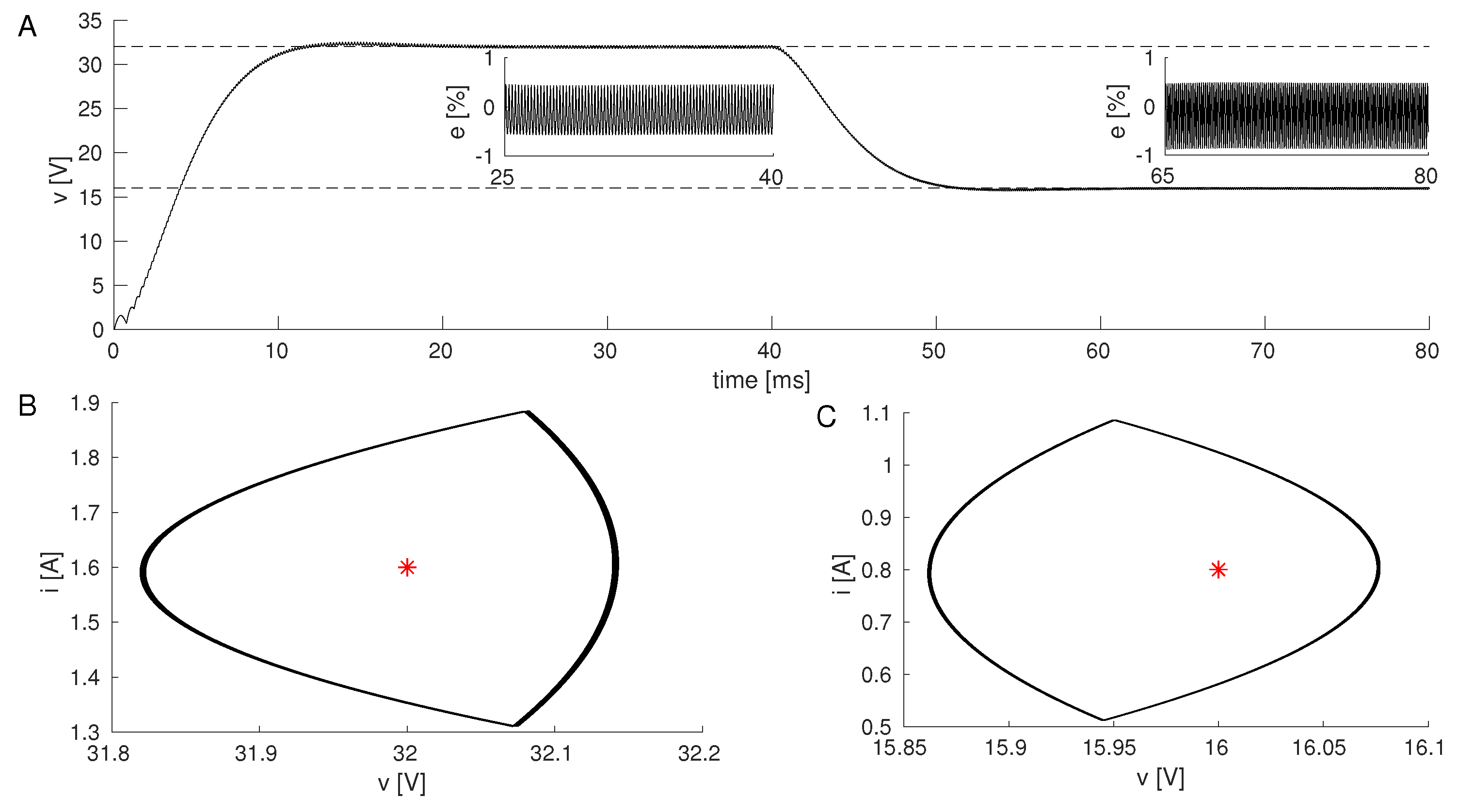
The results of the 3D system behavior and its ability to reject disturbances in the reference voltage are depicted in Figure 4. In this figure, a reference voltage of ${\overline{v}}_{ref}=32$ V is applied during the first 40 ms of the simulation, after this, the reference voltage is drastically decreased by a $50\%$, i.e., ${\overline{v}}_{ref}=16$ V and the system is allowed to evolve during 40ms more. From Figure 4a it is possible to deduce that, in the 3D system, the controller is also able to regulate with a settling time of ≈ 10 ms and a steady state error smaller than $1\%$. Not only this, but also the control is robust against disturbances in the reference output value. Panel B,C of the same figure show the orbit exhibited by the system in the steady state before and after the disturbance, which clearly evolves in the neighborhood of the equilibrium value $({\overline{v}}_{ref},{\overline{i}}_{ref})$ (red star).

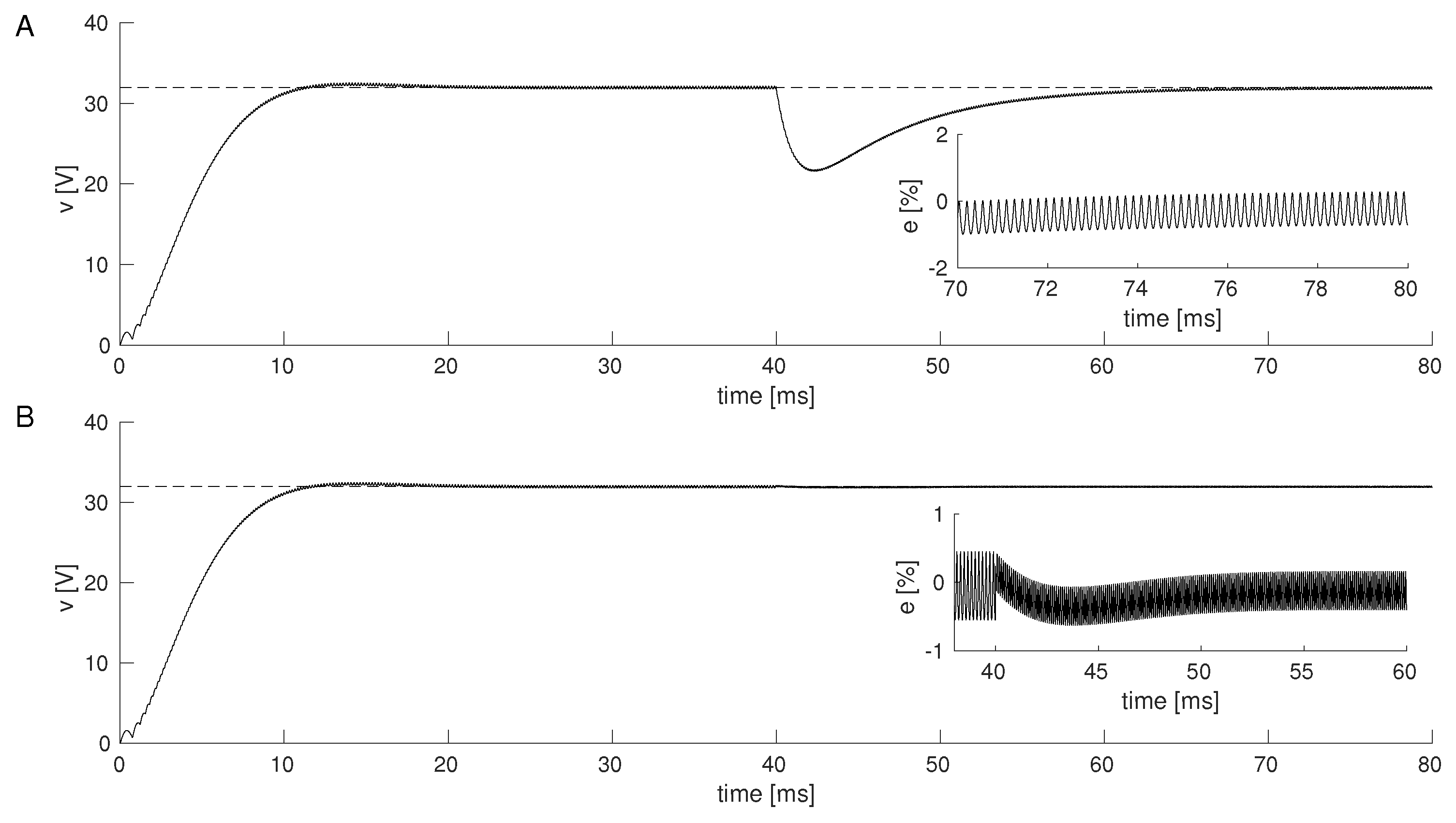
We also tested the capability of the system to reject disturbances both in the load R and the input voltage E. To do so we simulated a similar set-up to the one described for the 2D system. In particular we evolved the unperturbed system during 40 ms to achieve a steady state, and immediately after the perturbation is presented. For Figure 5a the perturbation is induced as a sudden change in the load from $R=20\mathsf{\Omega }$ to $R=15\mathsf{\Omega }$ (25% change). As depicted in the main figure of the panel and its inset, the system recovers to the reference voltage ${\overline{v}}_{ref}=32$ V (dashed line) with a percentage error smaller than 1%. A similar scenario is plotted in Figure 5b, in this case the perturbation is presented as a change in the input voltage from $E=40$ V to $E=50$ V. Even though the perturbation in the input corresponds to a $25\%$ change, the system barely moves from its steady state, and the perturbation only induces a slight increase in the error. This small error, which is never larger than 1%, rapidly returns to the steady value after 10 ms. (see inset). An important aspect of the controller design is that the first two elements in the normal vector of the switching surface in Equation (33), are exactly those of Equation (21) for the 2D case, where neither the norm of the vectors nor $\delta$ were involved. Hence, the effect of $c_1/c_2$ and $\delta$ are only exhibited in the third term.

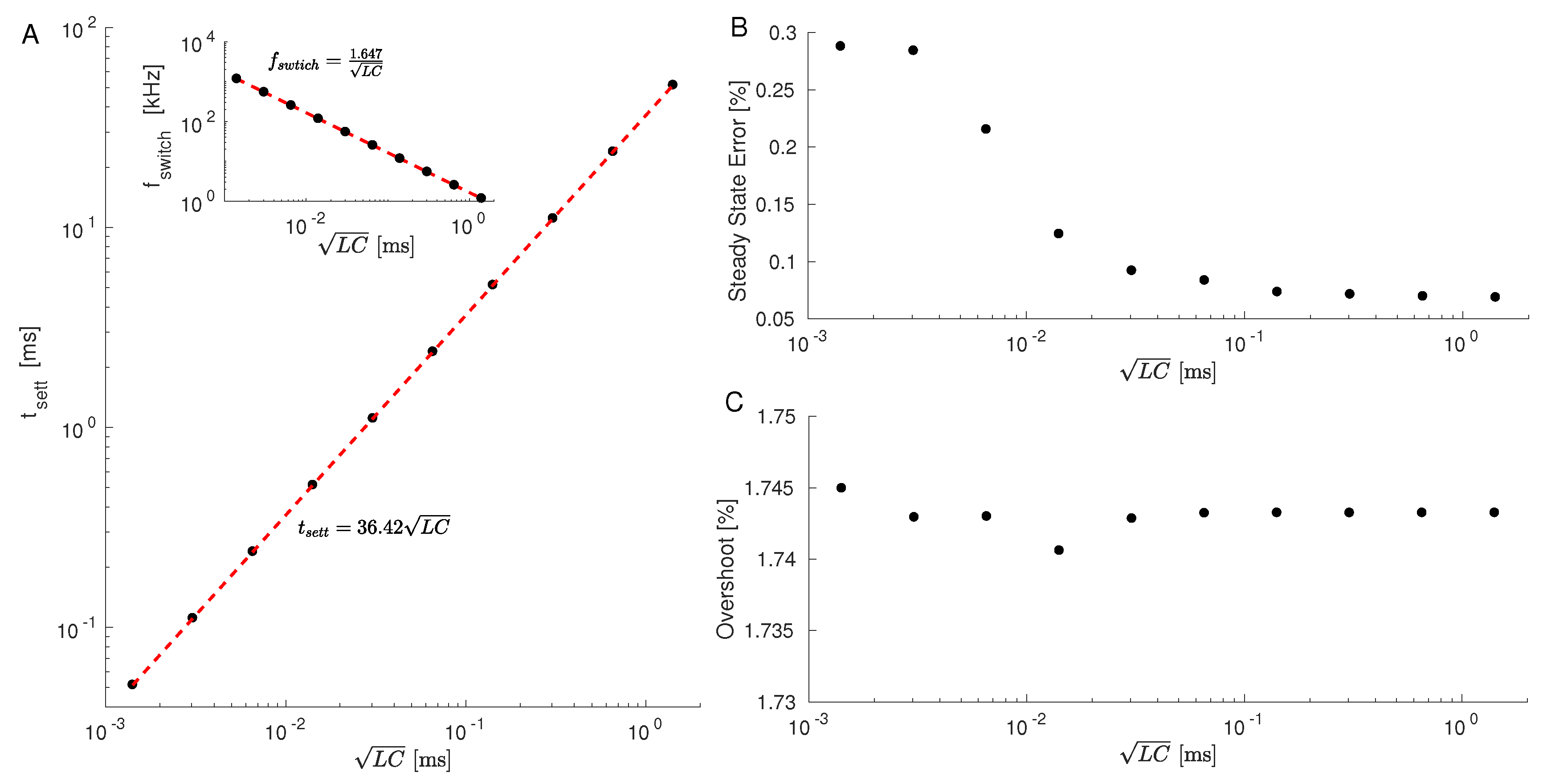
So far we have numerically analyzed the controller for a particular design of a buck converter determined by the values of the parameters R, L, C, and E and $v_{ref}$. However, as we demonstrated in Section 5, the methodology proposed here is general. To demonstrate this generality we performed simulations of our proposed controller under different values of parameters L and C which preserved the value of $\gamma \approx 0.3536$. To do so, we fixed the value of $R=20\mathsf{\Omega }$. Then the inductance was varied in the range $L=[20\mathsf{\mu }$H 10 mH] and the capacitance was automatically set to $C=L/50$ F. According to the normalization of the buck converter, this amounts to change the time scale $\sqrt{LC}$ in which the power converter evolves, while keeping the dynamical behavior invariant (recall that the actual dynamics of the normalized system only depend on the value of $\gamma$). The results of this analysis are reported in Figure 6. In particular, Figure 6a shows how the settling time changes when varying the time scale $\sqrt{LC}$. Not surprisingly, increasing values of $\sqrt{LC}$ produce a linearly increase also in the settling time, since the effect of the former is to stretch and compress the time in which the system evolves. The inset in this panel shows also how the switching frequency increases as the evolution of the system is faster (decreasing values of $\sqrt{LC}$). This behavior emerges since we have kept the hysteresis band $ϵ=\pm 0.05$, which highlights the need to use faster switches when trying to achieve faster dynamics. Finally we calculated also the average steady state error and the overshoot for each one of the $\sqrt{LC}$ values (see Figure 6b,c). On the one hand, the steady state error was always kept below 0.3%, regardless the time scale of the system. On the other hand, overshoot didn’t change significantly which supports again the claim that the dynamical behavior remains unchanged under this particular design criteria.

6. Conclusions and Future Work

In this paper we developed a switched control action for the buck power converter that guarantees global asymptotic stability, by applying recent results from contraction analysis. To do so, we took advantage of the Jordan canonical form of the system to fulfill the conditions of global stability resulting from contraction analysis, which wouldn’t have been met in the original form of the system. At first, we applied the design to the original 2D buck converter model where the controller presented good performance and robustness to voltage reference changes; however, as the load varied, regulation was lost. To overcome this issue, we extended the 2D-system to take into account the dynamics of the error inspired by the disturbance-rejection effect of a PI controller. With this design, the controlled system showed robustness to several types of disturbances including load and input voltage changes.

Although the 3D system is robust, it comes with the price of increasing the settling time respect to the 2D design. To overcome this issue, one can make use of a different buck converter design (different capacitance and/or inductance) to achieve the desired time-scale of the dynamics (which is mainly driven by the factor $\sqrt{LC}$) and then design the controller according to our methodology. It shall be noticed that other control techniques designed for the buck converter may show better performance in terms of efficiency, however, it is important to stress that the method outlined in this paper is not only simple in its implementation (design based on hysteresis band) but also quite general. This is because it is not based on the linearized version of the system but on the nonlinear form, such that the resulting controller is globally stable, a feature that cannot usually be guaranteed using linearization. Indeed we have numerically tested the globally stability property by performing extensive simulations for different initial conditions in the $(v,i,y)$ space. These tests showed convergence for all the simulations.

Throughout this paper we have analyzed and designed the controller assuming that the current flowing through the inductor is always positive, a topology known as Continuous Conduction Mode (CCM). Depending on the value of the load and disturbances in it, the buck converter can enter in Discontinuous Conduction Mode (DCM), where the current through the inductor is zero. The control design that we have provided in this paper only takes into consideration the dynamical behavior of the buck converter in CCM. Considering also DCM implies adding a further topology to the system (vector field) which implies the study of contraction in multimodal filippov systems. This issue is indeed a current topic of research in the field of applied mathematics.

Finally, whether the approach presented here can be applied to other power converters such as the boost, is currently an open problem. This is because not every single system can be easily approached by contraction theory and other standard tools for stability analysis might be the best option in these cases.

References

- Chen, S.M.; Wang, C.Y.; Liang, T.J. A novel sinusoidal boost-flyback CCM/DCM DC-DC converter. In Proceedings of the 2014 IEEE Applied Power Electronics Conference and Exposition–APEC, Fort Worth, TX, USA, 16–20 March 2014; pp. 3512–3516. [Google Scholar]
- Tseng, K.C.; Lin, J.T.; Cheng, C.A. An Integrated Derived Boost-Flyback Converter for fuel cell hybrid electric vehicles. In Proceedings of the 2013 1st International Future Energy Electronics Conference (IFEEC), Tainan, Taiwan, 3–6 November 2013; pp. 283–287. [Google Scholar]
- Siouane, S.; Jovanovic, S.; Poure, P. Service Continuity of PV Synchronous Buck/Buck-Boost Converter with Energy Storage. Energies 2018, 11, 1369. [Google Scholar] [CrossRef]
- Ortigoza, R.S.; Rodriguez, V.H.G.; Marquez, E.H.; Ponce, M.; Sanchez, J.R.G.; Juarez, J.N.A.; Ortigoza, G.S.; Perez, J.H. A Trajectory Tracking Control for a Boost Converter-Inverter-DC Motor Combination. IEEE Lat. Am. Trans. 2018, 16, 1008–1014. [Google Scholar] [CrossRef]
- Fernando, W.A.; Lu, D.D. Bi-directional converter for interfacing appliances with HFAC enabled power distribution systems in critical applications. In Proceedings of the 2017 20th International Conference on Electrical Machines and Systems (ICEMS), Sydney, Australia, 11–14 August 2017; pp. 1–6. [Google Scholar] [CrossRef]
- Singh, S.; Singh, B.; Bhuvaneswari, G.; Bist, V. A Power Quality Improved Bridgeless Converter-Based Computer Power Supply. IEEE Trans. Ind. Appl. 2016, 52, 4385–4394. [Google Scholar] [CrossRef]
- Undeland, T.M.; Robbins, W.P.; Mohan, N. Power Electronics: Converters, Applications, and Design; John Wiley and Sons: New York, NY, USA, 2003. [Google Scholar]
- Erickson, R.W.; Maksimović, D. Fundamentals of Power Electronics; Springer: Berlin, Germany, 2001. [Google Scholar]
- Mueller, J.A.; Kimball, J. Modeling Dual Active Bridge Converters in DC Distribution Systems. IEEE Trans. Power Electron. 2018. [Google Scholar] [CrossRef]
- Banerjee, S.; Verghese, G.C. Nonlinear Phenomena in Power Electronics: Attractors, Bifurcations, Chaos, and Nonlinear Control; IEEE Press: New York, NY, USA, 2001. [Google Scholar]
- Cheng, C.H.; Cheng, P.J.; Xie, M.J. Current sharing of paralleled DC–DC converters using GA-based PID controllers. Expert Syst. Appl. 2010, 37, 733–740. [Google Scholar] [CrossRef]
- Guo, L.; Hung, J.Y.; Nelms, R.M. Evaluation of DSP-Based PID and Fuzzy Controllers for DC-DC Converters. IEEE Trans. Ind. Electron. 2009, 56, 2237–2248. [Google Scholar]
- Rodríguez-Licea, M.A.; Pérez-Pinal, F.J.; Nuñez-Perez, J.C.; Herrera-Ramirez, C.A. Nonlinear Robust Control for Low Voltage Direct-Current Residential Microgrids with Constant Power Loads. Energies 2018, 11, 1130. [Google Scholar] [CrossRef]
- Aguilera, R.P.; Quevedo, D.E. Predictive Control of Power Converters: Designs With Guaranteed Performance. IEEE Trans. Ind. Inf. 2015, 11, 53–63. [Google Scholar] [CrossRef]
- Alsmadi, Y.M.; Utkin, V.; Haj-ahmed, M.A.; Xu, L. Sliding mode control of power converters: DC/DC converters. Int. J. Control 2017. [Google Scholar] [CrossRef]
- Khaligh, A.; Rahimi, A.M.; Emadi, A. Modified Pulse-Adjustment Technique to Control DC/DC Converters Driving Variable Constant-Power Loads. IEEE Trans. Ind. Electron. 2008, 55, 1133–1146. [Google Scholar] [CrossRef]
- Gabian, G.; Gamble, J.; Blalock, B.; Costinett, D. Hybrid buck converter optimization and comparison for smart phone integrated battery chargers. In Proceedings of the 2018 IEEE Applied Power Electronics Conference and Exposition (APEC), San Antonio, TX, USA, 4–8 March 2018; pp. 2148–2154. [Google Scholar]
- Lai, C.; Cheng, Y.; Hsieh, M.; Lin, Y. Development of a Bidirectional DC/DC Converter With Dual-Battery Energy Storage for Hybrid Electric Vehicle System. IEEE Trans. Veh. Technol. 2018, 67, 1036–1052. [Google Scholar] [CrossRef]
- Lukmana, M.A.; Nurhadi, H. Preliminary study on Unmanned Aerial Vehicle (UAV) Quadcopter using PID controller. In Proceedings of the 2015 International Conference on Advanced Mechatronics, Intelligent Manufacture, and Industrial Automation (ICAMIMIA), Surabaya, Indonesia, 15–17 October 2015; pp. 34–37. [Google Scholar] [CrossRef]
- Chiang, C.; Chen, C. Zero-Voltage-Switching Control for a PWM Buck Converter Under DCM/CCM Boundary. IEEE Trans. Power Electron. 2009, 24, 2120–2126. [Google Scholar] [CrossRef]
- Calderón, A.; Vinagre, B.; Feliu, V. Fractional order control strategies for power electronic buck converters. Signal Process. 2006, 86, 2803–2819. [Google Scholar] [CrossRef]
- Suh, J.; Seok, J.; Kong, B. A Fast Response PWM Buck Converter with Active Ramp Tracking Control in Load Transient period. IEEE Trans. Circuits Syst. II Express Briefs 2018. [Google Scholar] [CrossRef]
- Chang, C.; Yuan, Y.; Jiang, T.; Zhou, Z. Field programmable gate array implementation of a single-input fuzzy proportional-integral-derivative controller for DC-DC buck converters. IET Power Electron. 2016, 9, 1259–1266. [Google Scholar] [CrossRef]
- El Aroudi, A.; Giaouris, D.; Iu, H.H.C.; Hiskens, I.A. A review on stability analysis methods for switching mode power converters. IEEE J. Emerg. Sel. Top. Circuits Syst. 2015, 5, 302–315. [Google Scholar] [CrossRef]
- Fiore, D.; Hogan, S.J.; di Bernardo, M. Contraction analysis of switched systems via regularization. Automatica 2016, 73, 279–288. [Google Scholar] [CrossRef] [Green Version]
- di Bernardo, M.; Fiore, D. Switching control for incremental stabilization of nonlinear systems via contraction theory. In Proceedings of the 2016 European Control Conference (ECC), Aalborg, Denmark, 29 June–1 July 2016; pp. 2054–2059. [Google Scholar] [CrossRef]
- Lohmiller, W.; Slotine, J.J.E. On Contraction Analysis for Non-linear Systems. Automatica 1998, 34, 683–696. [Google Scholar] [CrossRef] [Green Version]
- Chen, C.T. Linear Systems Theory and dEsign; Oxford University Press: Oxford, UK, 1999. [Google Scholar]
- Vidyasagar, M. Nonlinear Systems Analysis; Prentice Hall: Englewood Cliffs, NJ, USA, 1993. [Google Scholar]
- Slotine, J.J.E.; Li, W. Applied Nonlinear Control; Prentice Hall: Englewood Cliffs, NJ, USA, 1991; Volume 199. [Google Scholar]
- Khalil, H.K. Nonlinear Control; Pearson: New York, NY, USA, 2015. [Google Scholar]
- Deane, J.H.; Hamill, D.C. Analysis, simulation and experimental study of chaos in the buck converter. In Proceedings of the PESC’90 Record 21st Annual IEEE Power Electronics Specialists Conference, San Antonio, TX, USA, 11–14 June 1990; pp. 491–498. [Google Scholar]
- Fossas, E.; Olivar, G. Study of chaos in the buck converter. IEEE Trans. Circuits Syst. I Fundam. Theory Appl. 1996, 43, 13–25. [Google Scholar] [CrossRef] [Green Version]
Figure 1.
Schematic diagram of a buck power converter.
Figure 2.
(A) Time trace of the voltage in the capacitor v. During the first 30 ms a V is used, after this a drastic change to V is applied (depicted in the dashed lines). The time trace of the steady state percentage error is also depicted in the insets for both values of ; (B) Phase representation of the steady state for ; (C) , with the equilibrium point indicated by the red star. Simulations were performed using MATLAB® with a fourth order Runge-Kutta algorithm with variable step and event detection to identify collisions with the hysteresis band. Steady state was considered after 20 ms of simulation time. Initial conditions were chosen as . Other parameters as in the main text.
Figure 3.
Time response of the capacitor’s voltage v. During the first 30 ms, the value of the resistor is set to , after this the load is changed to . Inset: Steady state percentage error (considered 15 ms after the presentation of the disturbance). The desired output is plot with the dashed line. Other details as in Figure 2.
Figure 4.
(a) Time trace of the voltage in the capacitor v. During the first 40 ms a V is used, after this a drastic change to V is applied (depicted in the dashed lines). The time trace of the steady state percentage error is also depicted in the insets for both values of ; (b) Phase representation of the steady state for ; (c) , with the equilibrium point indicated by the red star. This results were obtained by making and . Steady state was considered after 25 ms of transient dynamics. Other parameters as in the main text and Figure 2.
Figure 5.
(a) Time response of the capacitor’s voltage v. During the first 40ms, the value of the resistor is set to , after this the load is changed to . Inset: Steady state percentage error (considered 25 ms after the presentation of the disturbance). The desired output is plot with the dashed line; (b) Same as (A) for a disturbance in the input voltage E. During the first 40 ms V, after this it is changed to V. In this panel, the inset shows the percentage error during the first 20 ms after the presentation of the input disturbance. Other details as in Figure 2.
Figure 6.
(A) Black symbols: Settling time of the buck converter with different values of and fixed , preserving the value of . Red line: Linear fit of the simulation points. For this plot, we chose inductance values in the range H 10 mH] and a capacitance F. Settling time was calculated as the time it takes to the system to evolve from to the point in which the error doesn’t leave the band. Inset: Switching frequency resulting from the hysteresis band in Equation (33) for the different values of reported in the main figure (black symbols). Red line depicts the fitted function reported in the text box; (B) Average steady state error calculated as the mean value of the error after the settling time; (C) percentage overshoot for the values of reported in panel (A). For each simulation point, the system is evolved during a time span of . Other details as in Figure 2.
© 2018 by the authors. Licensee MDPI, Basel, Switzerland. This article is an open access article distributed under the terms and conditions of the Creative Commons Attribution (CC BY) license (http://creativecommons.org/licenses/by/4.0/).
Share and Cite
MDPI and ACS Style
Angulo-Garcia, D.; Angulo, F.; Osorio, G.; Olivar, G. Control of a DC-DC Buck Converter through Contraction Techniques. Energies 2018, 11, 3086. https://doi.org/10.3390/en11113086
AMA Style
Angulo-Garcia D, Angulo F, Osorio G, Olivar G. Control of a DC-DC Buck Converter through Contraction Techniques. Energies. 2018; 11(11):3086. https://doi.org/10.3390/en11113086
Chicago/Turabian StyleAngulo-Garcia, David, Fabiola Angulo, Gustavo Osorio, and Gerard Olivar. 2018. "Control of a DC-DC Buck Converter through Contraction Techniques" Energies 11, no. 11: 3086. https://doi.org/10.3390/en11113086
Note that from the first issue of 2016, this journal uses article numbers instead of page numbers. See further details here.