Multi-Step Short-Term Power Consumption Forecasting with a Hybrid Deep Learning Strategy


1
Key Laboratory of Electromagnetic Wave Information Technology and Metrology of Zhejiang Province, College of Information Engineering, China Jiliang University, Hangzhou 310018, China
2
Department of Electrical and Electronic Engineering, Xi’an Jiaotong-Liverpool University, Suzhou 215123, China
3
State Grid Zhejiang Electric Power Co., Ltd, Hangzhou 310007, China
*
Author to whom correspondence should be addressed.
Energies 2018, 11(11), 3089; https://doi.org/10.3390/en11113089
Submission received: 30 September 2018
/
Revised: 31 October 2018
/
Accepted: 7 November 2018
/
Published: 8 November 2018
(This article belongs to the Special Issue Intelligent Control in Energy Systems)
Abstract
:Electric power consumption short-term forecasting for individual households is an important and challenging topic in the fields of AI-enhanced energy saving, smart grid planning, sustainable energy usage and electricity market bidding system design. Due to the variability of each household’s personalized activity, difficulties exist for traditional methods, such as auto-regressive moving average models, machine learning methods and non-deep neural networks, to provide accurate prediction for single household electric power consumption. Recent works show that the long short term memory (LSTM) neural network outperforms most of those traditional methods for power consumption forecasting problems. Nevertheless, two research gaps remain as unsolved problems in the literature. First, the prediction accuracy is still not reaching the practical level for real-world industrial applications. Second, most existing works only work on the one-step forecasting problem; the forecasting time is too short for practical usage. In this study, a hybrid deep learning neural network framework that combines convolutional neural network (CNN) with LSTM is proposed to further improve the prediction accuracy. The original short-term forecasting strategy is extended to a multi-step forecasting strategy to introduce more response time for electricity market bidding. Five real-world household power consumption datasets are studied, the proposed hybrid deep learning neural network outperforms most of the existing approaches, including auto-regressive integrated moving average (ARIMA) model, persistent model, support vector regression (SVR) and LSTM alone. In addition, we show a k-step power consumption forecasting strategy to promote the proposed framework for real-world application usage.
1. Introduction
Artificial intelligence (AI) enhanced electric power consumption short-term forecasting is an important technique for smart grid planning, sustainable energy usage and electricity market bidding system design. Existing work shows that 20% extra energy output is required to overcome a 5% integrated residential electric power consumption peak increment without effective power consumption forecasting [1]. The advanced metering infrastructure (AMI) introduces the possibility to learn power consumption pattern for each residential house from its historical data. The resulting power consumption prediction provides an important hint for both the power suppliers and consumers to maintain a sustainable environment for energy saving, management and scheduling [2,3].
Efficient and precise power consumption forecasting is always demanded in dynamic electricity market bidding system design [4,5,6]. However, both manual or automated power bidding requires response time for computerized calculation. Most existing works only perform one-step power load forecasting, which enquire immediate response from the participants. A multi-step forecasting strategy can be more preferred under this situation. In summary, for individual household electric power consumption prediction, two main challenges exist in the literature:
- High prediction accuracy. The volatility level of single household power consumption is high due to the irregular human behaviours. Moreover, the source data is usually univariate, consisting only power consumption records in kilowatts (kws), which increases the difficulty for accurate power consumption forecasting.
- Multi-step forecasting. Most existing load forecasting works focus on one-step forecasting solutions. A longer time forecasting solution is required to facilitate real-world application usage, such as the dynamic electricity market bidding system design.
Traditional electric power forecasting methods overcome the uncertainty by integrating the overall power consumption of a large group of households or clustering similar pattern customers into sub-groups to reduce the irregularity. However, during the development process of smart grid, the accurate prediction of a household electric power consumption is highly demanded, which may come out with a customized electricity price plan for that particular household. Moreover, univariate data forecasting remains as one of the most challenging problems in the field of machine learning, since most of the dependent variables are unknown, such as the electric current, voltage, weather conditions, etc. [7]. Classic univariate forecasting methods are usually applied to cases that either the rest of the features are too difficult to be measured or there are too many variables to be measured, e.g., the stock market indices forecasting problems [8]. Flexibility of those univariate forecasting methods is introduced while no extra information is required. The proposed approach can be plugged into management system for other households power consumption forecasting as long as the historical data is available in the system.
In recent years, deep learning neural networks (DLNNs) became increasingly attractive throughout the world and were extensively employed in a large number of application fields, including natural language processing (NLP) [9], image object detection [10], time series analysis [11], etc. For individual household power consumption forecasting problems, recent works reported that the long short term memory (LSTM) neural network provides extremely high accuracy on prediction [2,12,13]. Experimental results show that, by using the conventional LSTM neural network alone, the prediction accuracy outperforms most of the traditional statistical and machine learning methods, including auto-regressive integrated moving average (ARIMA) model [14], support vector machine (SVM) [15], non-deep artificial neural networks (ANNs) [16] and their combinations [17], because of the extra neighboring time frame states dependencies introduced by memory gates in recurrent neural network (RNN). However, even recent works, such as [2,12,13] focus on short-term forecasting strategy, which forecast power load only one step further. For particular applications, such as electricity market bidding system design, a longer time forecasting strategy can be more preferred.
Moreover, LSTM neural network is a special form of RNN [18]; and there exist other types of DLNNs, such as convolution neural networks (CNNs) [19] and deep belief nets (DBNs) [20]. The temporal CNN, which consists of a special 1-D convolution operation, is also reported to be potentially useful for time series prediction problems [21]. In the field of NLP, there are suggestions to combine the temporal CNN with RNN to obtain more precise classification results [22].
1.1. Related Works
Electric power consumption forecasting is useful in many application areas. Besides electricity market bidding, it can also be applied to demand side management for transcative grid [3] and power ramp rate control [23]. Conventional forecasting methods include support vector regression (SVR), ANNs, fuzzy logic methods [24] and time series analysis methods, such as autoregressive integrated moving average (ARIMA) [25], autoregressive method with exogenous variables [26,27] and grey models (GMs) [28]. As early as 2007, Ediger and Akar [29] started to use ARIMA and seasonal ARIMA methods to forecast the energy consumption by fuel until the year 2020 in Turkey. Yuan et al. [14] compared the results of China’s primary energy consumption forecasting using ARIMA and GM (1,1). Both methods work well; and a hybrid method combining the two methods was also proposed to show the best mean absolute percent error (MAPE) value they could achieve. Oğcu et al. [30] compared ANN and support vector regression (SVR) models in forecasting electricity consumption of Turkey. For performance measurement, the mean absolute percentage error (MAPE) rates are used; and the SVR model showed a 0.6% better performance than ANN. Rodrigues et al. [31] designed an ANN energy consumption model consisting of a single hidden layer with 20 neurons to forecast 93 households energy consumptions in Portugal. Experimental results showed an averaged MAPE value of 4.2% for daily energy consumption forecasting in between of the 93 households. Deb et al. [32] compared ANN and an adaptive neuro-fuzzy interface system for energy consumption forecasting of three institution buildings in Singapore, and showed high forecasting accuracy. Wang and Hu [33] proposed hybrid forecasting method combining ARIMA model, extreme learning machine (ELM), SVRs and Gaussian process regression model for short-term wind speed forecasting problem. All individual base forecasting models are integrated in a non-linear way, where the experimental results showed the forecasting accuracy and reliability of the proposed hybrid method.
Deep learning neural networks are modern popular machine learning techniques dealing with big data with high classification and prediction accuracy, which has been widely applied in many fields, such as stock indices forecasting [34,35], wind speed prediction [36,37], solar irradiance forecasting [38,39], etc. In recent years, with the fast development of smart grid technology, DLNNs are widely employed to solve power consumption forecasting problems, both for industrial and residential buildings; and because of the significantly more internal hidden layers and computations compared to classic ANNs, DLNN is applied to more challenging problems, such as power consumption forecasting for individual households [21]. Ryu et al. [40] trained DLNN with single household electricity consumption data in 2016 and showed that the DLNN can produce better prediction accuracy compared with shallow neural network (SNN), double seasonal Holt–Winters (DSHW) model and the autoregressive integrated moving average (ARIMA). Shi et al. [12] proposed a pooling-based deep recurrent neural network to capture the uncertainty of single household load forecasting problem and applied the proposed method on 920 Ireland customers’ smart meter data. Experimental results show that the proposed deep learning neural network outperforms most classic data-driven forecasting methods, including ARIMA, SVR and RNN. Kong et al. [13] straightly applied a two-hidden-layer LSTM to single household power consumption forecasting problems; and compared their results with back-propagation neural network (BPNN), k-nearest neighbor regression (KNN) and extreme learning machine (ELM) to show the large forecasting accuracy improvement by using LSTM.
1.2. Contributions
In this study, a hybrid deep learning neural network framework combining LSTM neural network with CNN is designed to deal with the single household power consumption forecasting problem. The conventional LSTM neural network is extended by adding a pre-processing phase using CNN. The pre-processing phase extracts useful features from the original data and more importantly, converts the univariate data into multi-dimensional by 1-D convolution, which potentially enhances the prediction capability of the LSTM neural network. To evaluate the performance of the proposed framework, a series of experiments were performed based on five real-world households electric power consumption data collected by the UK-DALE dataset [41]. The experimental results show that the proposed hybrid DLNN framework outperforms most of the existing approaches in the literature, including auto-regressive integrated moving average (ARIMA) model, support vector regression (SVR) and LSTM alone with three measurement metrics, including root-mean-square error (RMSE), mean absolute error (MAE) and mean absolute percentage error (MAPE). The scientific impacts of this work to the literature involve:
- A 1-D convolutional neural network is introduced to pre-process the univariate dataset and convert the original data into multi-dimensional features after two layers of temporal convolution operations.
- A hybrid deep neural network is designed to forecasting power consumption for individual household. Experimental results show that the proposed framework outperforms most of the existing approaches including ARIMA, SVR and LSTM.
- A k-step forecasting strategy is designed to introduce k forecasting points/values simultaneously. The value of k is determined to be less than or equal to the number of cores/threads to maintain the efficiency. The actual forecasting period/response time depends on the power consumption recording interval and the value of k. Compared with traditional one-step forecasting strategies, the k-step forecasting solution provides more response time for dynamic electricity market bidding.
Five individual households located in UK are studied to show the effectiveness and robustness of the proposed hybrid DLNN structure design. The study of multi-step electric power consumption forecasting strategy can be useful in customizing the smart grid planning and electricity market bidding system design.
2. Materials and Methods
Long short term memory (LSTM) and convolutional neural network (CNN) are two hot branches of deep learning neural network and they have attracted wide attention across the world in recent years. In this study, aiming at solving the high volatility and uncertainty of single household power consumption forecasting problem, we combine LSTM and CNN to form a hybrid deep learning approach that is able to provide more accurate and robust forecasting result compared with traditional approaches.
With five real-world household power consumption data, the proposed framework pre-processes the raw data with CNN and uses the output of CNN to train the LSTM model.
2.1. Data Description
The power consumption data collected from five households located in London, UK was original published by Kelly and Knottenbelt [41]. In the original dataset, smart meters are used to collect power consumption data from each individual electric power device, such as television, air-con, fridge and so on. We utilize the aggregate power consumption data for the five households only. The original collection frequency is 6 s. We merge the data to convert it to time series datasets with time intervals at 5 min. Since the data lengths vary from different households, we select a continuous time period consisting of 12,000 data samples for each household. Out of 12,000 data samples, 10,800 data samples are used to train the proposed DLNN framework; and the remaining 1,200 data samples are retained for testing and verification purposes for each household.
2.2. Long Short Term Memory based Recurrent Neural Network
Long short term memory (LSTM) model is a special form of the recurrent neural network (RNN) that provides feedback at each neuron. The output of RNN is not only dependent on the current neuron input and weight but also dependent on previous neuron inputs. Therefore, theoretically speaking, the RNN structure is typically suitable for processing time series data. However, when dealing with a long and correlated series of data samples, exploding and vanishing gradients problems appear [42], which later becomes the cutting point for LSTM model to be introduced [43].
To overcome the vanishing gradients problem of RNN model, LSTM contains internal loops that maintain useful information and abandon garbages. There are four important elements in the flowchart of LSTM model: cell status, input gate, forget gate and output gate (Figure 1). The input, forget and output gates are used to control the update, maintenance and deletion of information contained in cell status. The forward computation process can be denoted as:
where , and represent current cell status value, last time frame cell status value and the update for the current cell status value, respectively. The notations , and represent forget gate, input gate and output gate, respectively. With proper parameter settings, the output value is calculated based on and values according to Equations (4) and (6). All weights, including: , , and , are updated based on the difference between the output value and the actual value following back-propagation through time (BPTT) algorithm [44].
2.3. Temporal Convolutional Neural Network
Convolutional neural network (CNN) is probably the most commonly used deep learning neural network which is currently mainly applied to image recognition/classification topics in the field of computer vision. With a large quantity of input raw data samples, CNN is usually capable to extract useful subsets of the input data efficiently. Generally speaking, CNN is still a feed-forward neural network, which is extended from multi-layer neural network (MLNN). The main difference between CNN and the traditional MLNN is that CNN has the properties of sparse interaction and parameter sharing [45].
Traditional MLNN uses full connection strategy to build the neural network between input layer and output layer, which means that each output neuron has the chance to interact with each input neuron. Suppose that there are m inputs and n outputs, the weight matrix has entries. CNN reduces the weight matrix size from to by setting up a convolutional kernel with size . Moreover, the convolutional kernel is shared by all inputs, which means that there is only one weight matrix with size to be learned from the training process. The two properties of CNN increases the training efficiency for parameter optimization; under the same computational complexity, the CNN is able to train a neural network with more hidden layers, or, in other words, a deeper neural network.
Temporal convolutional neural network introduces a special 1-D convolution, which is suitable for processing univariate time series data. Instead of using a convolutional kernel as in the traditional CNN, the temporal CNN uses a kernel size of . Suppose that the input data fits function ; the convolutional kernel function is . The 1-D convolution mapping between the input and kernel with step size d can be written as:
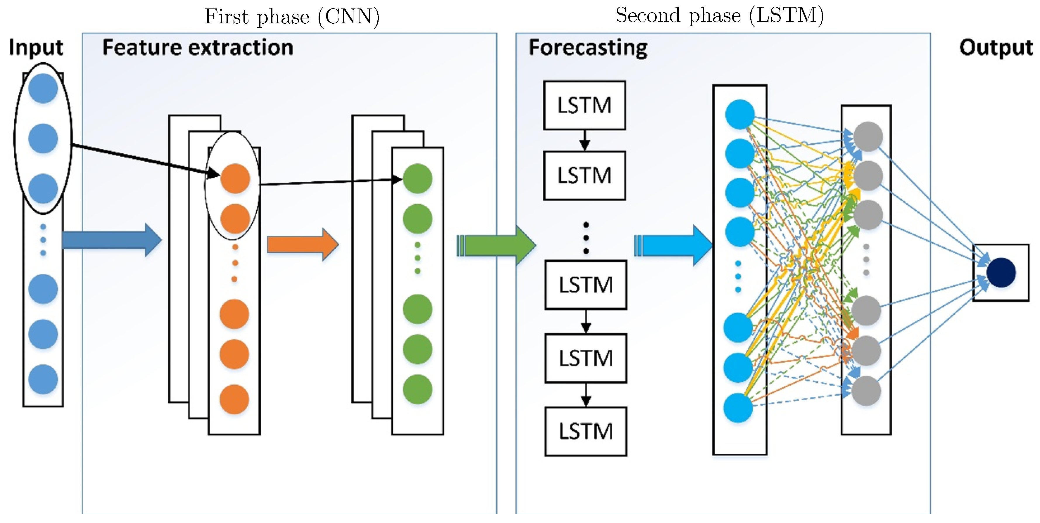
After the temporal convolutional operation, the original univariate dataset can be expanded to a m-dimensional feature dataset. In this way, the temporal CNN applies 1-D convolution to time series data and expand the univariate dataset to multi-dimensional extracted features (first phase in Figure 2); and the expanded features are found to be more suitable for prediction using LSTM.
2.4. CNN-LSTM Forecasting Framework
To attack the two challenges (volatility and univariate data) that we mentioned in Section 1, a hybrid deep neural network (DNN) combining CNN with LSTM is proposed. The structure of the hybrid DNN framework is depicted in Figure 2. In the pre-processing phase, CNN extract important information from the input data and most importantly, re-organize the univariate input data to multi-dimensional batches using convolution (Figure 2). In the second phase, the re-organized batches are input into LSTM units to perform forecasting.
From Figure 2, a two-hidden-layer temporal CNN is used to pre-process the input dataset. It is noted that the traditional temporal CNN usually includes pooling operations to prevent over-fitting when the number of hidden layer is greater than five. In this study, we omit the pooling operation to maximally retain the extracted features.
After pre-processing the input data, a LSTM neural network is designed to train and forecast the power consumption for individual household. The training process of LSTM structure is shown in Figure 3, where the extracted features from the first phase are treated as inputs to train the LSTM model. A dropout layer is added to the LSTM neural network to prevent overfitting. The loss value, which is the difference between the predicted output and the expected output , is computed to optimize the weights of all LSTM units. The optimization process follows the gradient descent optimization algorithm named RMSprop, which is commonly used for weight optimization of deep neural networks [46].
2.5. A k-Step Power Consumption Forecasting Strategy
Traditional power consumption forecasting approaches focus on one-step forecasting solutions [2,12,13]. For very short step size, such as 5 min, the response time can be too short for manual/automated electricity market bidding. In this study, we design a k-step power consumption forecasting strategy, which predicts k future data points simultaneously. Preassumption is made that the historical data is long enough to perform the data re-organization step.
Recall that the original power consumption data collected by UK-DALE has the step size at 6 s. The original data can be re-organized into different datasets with step size at n min, min, … min. In this study, we focus on . For each dataset, a core or a thread can be assigned to perform CNN-LSTM power consumption forecasting. The combinational result of all calculations from k cores provides a k-step power consumption forecasting solution, i.e., forecasting power consumption data points at 5 min, 10 min, … until 5k min in the future. Detailed algorithm of the proposed k-step power consumption forecasting strategy is shown in Algorithm 1.
| Algorithm 1 A k-step power consumption forecasting strategy |
Input: The UK-DALE dataset. Output: Data points at 5 min, 10 min, … 5k min. Initialization: re-organize the original data into k different datasets according to specified step sizes. While There are unassigned datasets and there are free threads/cores Assign any unassigned dataset to a free thread/core. Apply the proposed CNN-LSTM framework to the specific dataset and obtain one-step forecasting result. end-While Combine all one-step forecasting results to obtain a k-step power consumption forecasting result. |
Using the concurrent programming, we claim that the efficiency of the proposed k-step forecasting algorithm is competitive to the traditional one-step forecasting algorithms, given that the value of k is less than or equivalent to the number of threads/cores.
3. Results
The proposed hybrid DNN framework is implemented using Python 3.5.2 (64-bit) with PyCharm Community Edition 2016.3.2. The hardware configuration includes an Intel Core i7-7700 CPU @2.80GHz, 8G RAM and a NVIDIA GeForce GTX1050 graphics card. The proposed hybrid DNN framework is built based on the open source deep learning tool Tensorflow, proposed by Google [47] with Keras [48] version 2.0.8 as the front-end interface.
The prediction results of the proposed CNN-LSTM are compared with modern existing methods, including ARIMA model, SVR and LSTM. The prediction performances are evaluated using error metrics [49]. Three error metrics are calculated, including root-mean-square error (RMSE), mean absolute error (MAE) and mean absolute percentage error (MAPE). Generally speaking, smaller values of the error metrics present higher prediction accuracy. The formulations of the above three metrics are listed in Equations (7)–(9):
where is an actual testing sample value; is the prediction result of ; and N is the total number of testing samples.
All error metrics values of the five compared methods with all five households data described in Section 2.1 are listed in Table 1. The averaged computational time for each prediction point is recorded in Table 2 for all compared methods except the persistence model, since the persistence simply takes the previous time stamp’s data as the prediction result [50]. On average, and most of the cases in Table 1, the proposed CNN-LSTM framework outperforms all other compared forecasting methods with reasonable computational time (around 0.06 s for each prediction). Compared with SVR, the proposed framework has slightly higher MAE and RMSE values for households 2 and 4. From the data description of UK-DALE project, the power consumption curves of households 2 and 4 are less volatile; and the power consumption curves of households 1, 3 and 5 are relatively more active. The prediction results suggest that the deep learning methods are more suitable for volatile data description. Moreover, for MAPE, which measures the relative errors of the prediction results, the proposed CNN-LSTM framework shows lower error rates compared with all other methods for all five households.
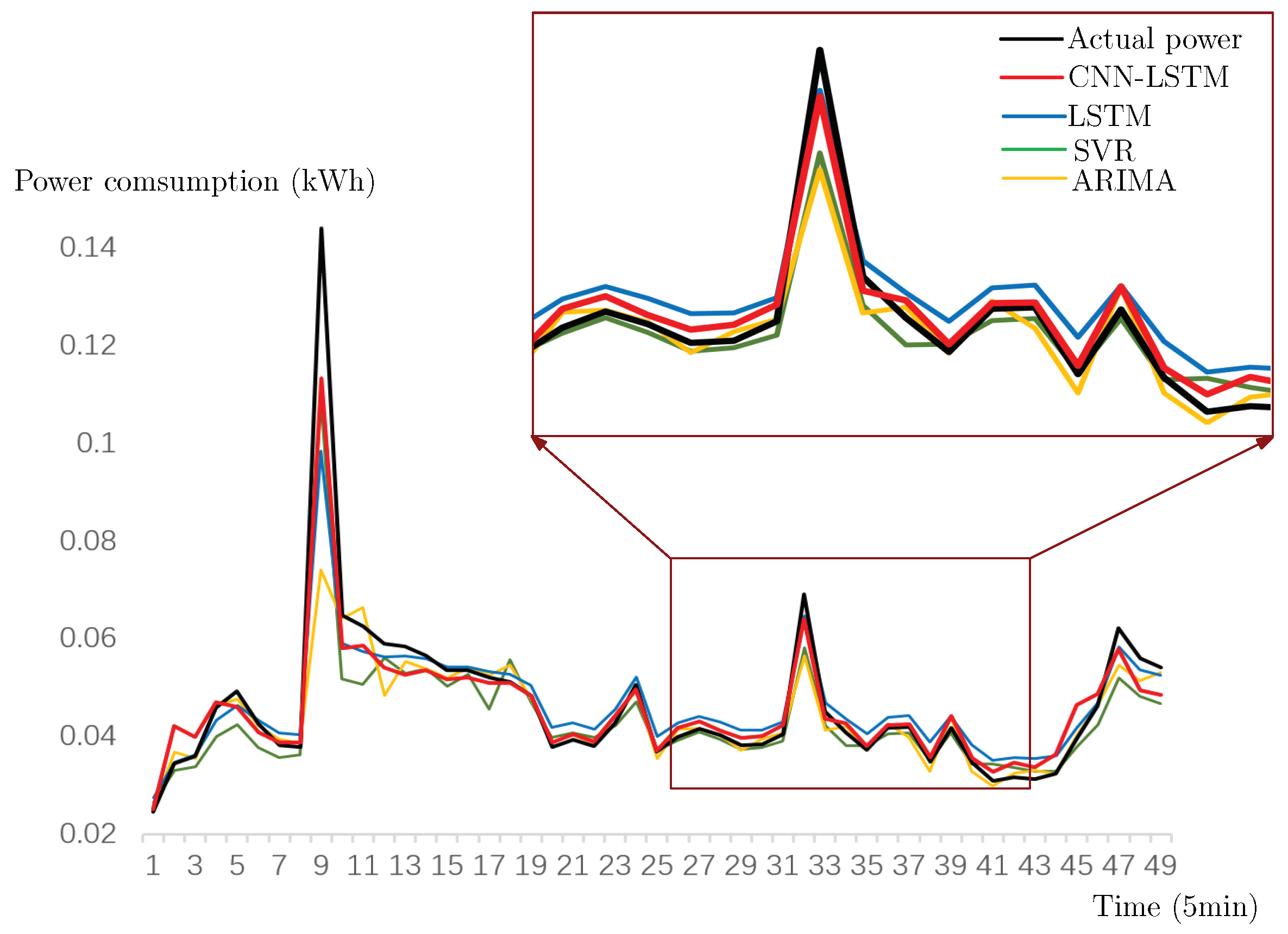
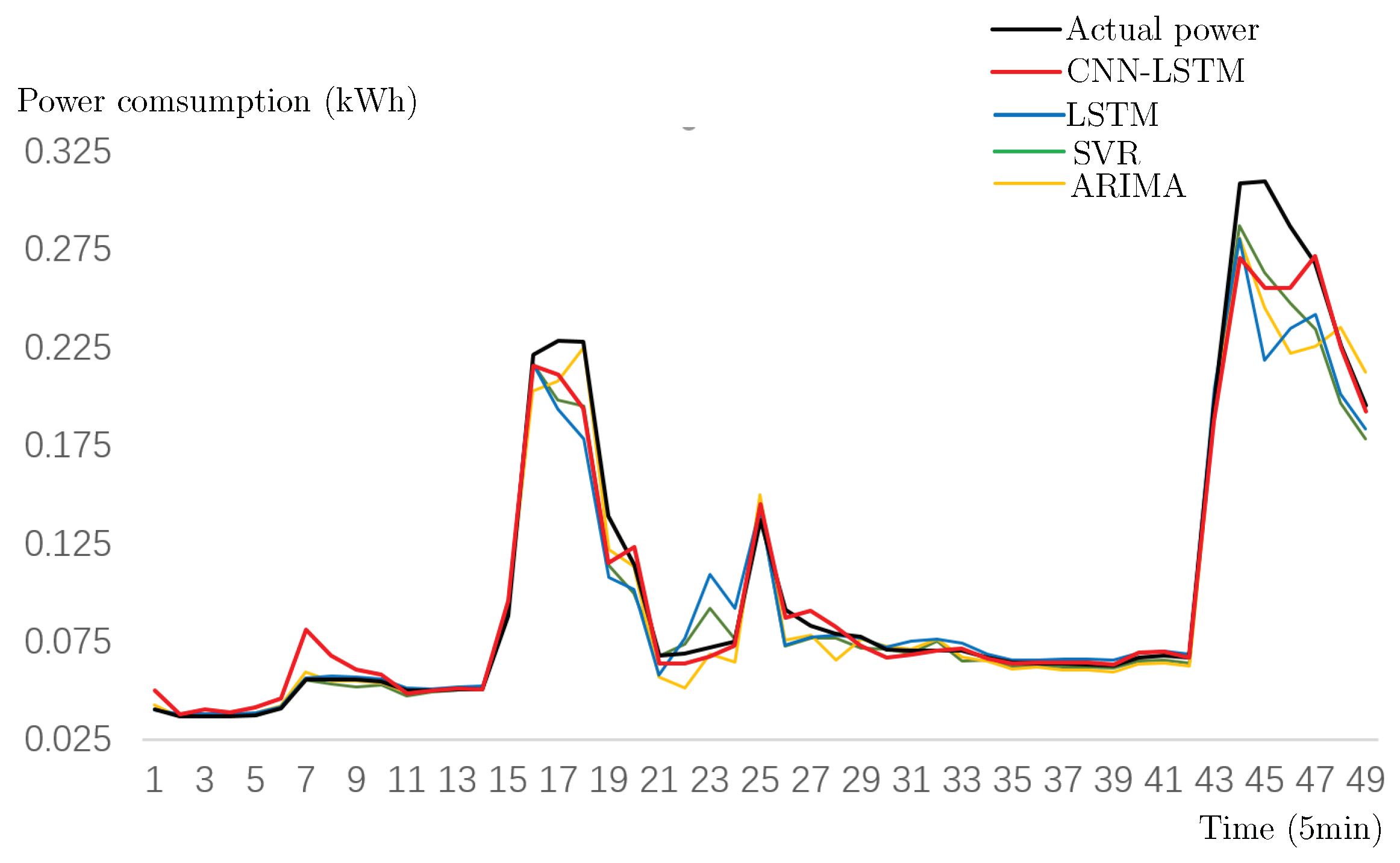
Figure 4, Figure 5 and Figure 6 show the detailed prediction results for households 1, 3 and 5. The actual power consumption curves are shown in black color; and the CNN-LSTM prediction results are shown in red. In general, from Figure 4, Figure 5 and Figure 6, the proposed CNN-LSTM method shows lower prediction errors and consequently higher prediction accuracy compared with ARIMA model, SVR and LSTM for all fives houses power consumption data collected by the UK-DALE dataset, which suggests that the proposed method is more robust than other methods for short-term power consumption forecasting.
In addition, we show the k-step power consumption forecasting results for k value up to 6. Table 3 shows RMSE and MAPE values for each house, while the value of k increases from 2 to 6. In Figure 7, twenty groups of 6-step power consumption forecasting results are depicted with training data omitted. It can be easily observed that the k-step forecasting algorithm produces more steps of forecasting results with acceptable compared to traditional one-step forecasting approaches.
Based on Algorithm 1, the k-step forecasting method repetitively runs the proposed CNN-LSTM framework. The average error and the average running time for the k-step algorithm will be very close to the original one-step CNN-LSTM framework, given that the value of k is less than or equivalent to the number of cores/threads.
Considering a very small power consumption interval at 5 min, the proposed method demonstrates a 30 min response time forecasting for dynamic electricity market bidding, which can be potentially useful in real-world applications [6]. The 30 min forecasting period is the necessary response time that we considered in this experimental section. Nevertheless, the 30 min response time can be further extended in two ways:
- First, the 5 × 6 = 30 min can be extended with larger k value. In order to keep our computation in real-time, we force the value of k to be less than or equivalent to the number of cores/threads. The response time can be extended with more powerful CPU.
- Second, the 5 × 6 = 30 min can also be extend using a coarser time interval, e.g., 15 min resolution instead of 5 min. For k = 6, the proposed k-step forecasting algorithm provides a one-and-a-half-hour response time for market bidding.
The project page and source code of the proposed CNN-LSTM framework is freely available online at: http://www.keddiyan.com/files/PowerForecast.html.
4. Conclusions and Future Work
This study proposed a novel hybrid deep learning neural network framework combining convolutional neural network (CNN) and long short term memory (LSTM) neural work to deal with univariate and volatile residential power consumption forecasting. Recent works already show that by LSTM neural network alone, high prediction accuracy for power consumption forecasting can be achieved [2,12,13]. We further demonstrate that the hybrid framework that was proposed in this study outperforms the conventional LSTM neural network. The CNN extracts the most useful information from the original raw data and converts the univariate single household power consumption dataset into multi-dimensional data, which potentially facilitates the prediction performance of LSTM.
Figure 8 shows the prediction accuracy improvement from conventional LSTM to CNN-LSTM using MAPE as a measurement metric. The results were obtained based on five real-world households power consumption data collected by the UK-DALE project. The proposed CNN-LSTM framework is 13.1%, 48.8%, 2.4%, 33.2% and 14.5% lower than LSTM, respectively, for the five tested households, using MAPE as the error metric, which demonstrates the usefulness of the proposed method for maintaining a sustainable balance between energy consumption and savings.
Instead of adopting the traditional one-step forecasting approaches, our method proposes a k-step forecasting algorithm for small step sizes, e.g., 6-step or 30 min forecasting period compared with the original 5 min short-term forecasting, to provide more response time for real-world applications, such as the electricity market bidding system design. The experimental results show the effectiveness for the proposed k-step forecasting algorithm for longer time period power consumption forecasting. The proposed approach can be further extended to deal with longer response time by varying different time interval resolutions and k values.
For the future work of this study, we intend to apply the proposed CNN-LSTM framework to more sophisticated real-world load datasets to verify the robustness of the proposed framework.
Author Contributions
Conceived and designed the algorithms: K.Y., X.W. and Y.D.; Performed the simulations: K.Y., X.W., N.J. and H.H.; Processed and Analyzed the data: X.W. and H.Z. Wrote the paper: K.Y., X.W.and Y.D.; Provide ideas to improve the computational approach: K.Y. and Y.D.
Funding
This work was supported by the National Natural Science Foundation of China (No. 61850410531, No. 61803315 and No. 61602431), research development fund of XJTLU (RDF-17-01-28), Key Program Special Fund in XJTLU (KSF-A-11), Jiangsu Science and Technology Program (SBK2018042034) and Zhejiang Provincial Basic Public Welfare Research Project (from Natural Science Foundation of Zhejiang Province) (No. LGF18F020017).
Conflicts of Interest
The authors declare no conflict of interest.
References
- Gyamfi, S.; Krumdieck, S. Scenario analysis of residential demand response at network peak periods. Electr. Power Syst. Res. 2012, 93, 32–38. [Google Scholar] [CrossRef] [Green Version]
- Kong, W.; Dong, Z.Y.; Hill, D.J.; Luo, F.; Xu, Y. Short-term residential load forecasting based on resident behaviour learning. IEEE Trans. Power Syst. 2018, 33, 1087–1088. [Google Scholar] [CrossRef]
- Chen, S.; Liu, C. From demand response to transactive energy: State of the art. J. Mod. Power Syst. Clean Energy 2017, 5, 10–19. [Google Scholar] [CrossRef]
- Gountis, V.P.; Bakirtzis, A.G. Bidding strategies for electricity producers in a competitive electricity marketplace. IEEE Trans. Power Syst. 2004, 19, 356–365. [Google Scholar] [CrossRef]
- Kian, A.R.; Cruz, J.B., Jr. Bidding strategies in dynamic electricity markets. Decis. Support Syst. 2005, 40, 543–551. [Google Scholar] [CrossRef]
- Siano, P. Demand response and smart grids—A survey. Renew. Sustain. Energy Rev. 2014, 30, 461–478. [Google Scholar] [CrossRef]
- Hu, M.; Ji, Z.; Yan, K.; Guo, Y.; Feng, X.; Gong, J.; Zhao, X.; Dong, L. Detecting anomalies in time deries fata via a meta-feature based approach. IEEE Access 2018, 6, 27760–27776. [Google Scholar] [CrossRef]
- Hsieh, T.J.; Hsiao, H.F.; Yeh, W.C. Forecasting stock markets using wavelet transforms and recurrent neural networks: An integrated system based on artificial bee colony algorithm. Appl. Soft Comput. 2011, 11, 2510–2525. [Google Scholar] [CrossRef]
- Socher, R.; Lin, C.C.; Manning, C.; Ng, A.Y. Parsing natural scenes and natural language with recursive neural networks. In Proceedings of the 28th International Conference on Machine Learning (ICML-11), Bellevue, WA, USA, 28 June–2 July 2011; pp. 129–136. [Google Scholar]
- Shao, L.; Cai, Z.; Liu, L.; Lu, K. Performance evaluation of deep feature learning for RGB-D image/video classification. Inform. Sci. 2017, 385, 266–283. [Google Scholar] [CrossRef]
- Kuremoto, T.; Kimura, S.; Kobayashi, K.; Obayashi, M. Time series forecasting using a deep belief network with restricted Boltzmann machines. Neurocomputing 2014, 137, 47–56. [Google Scholar] [CrossRef]
- Shi, H.; Xu, M.; Li, R. Deep learning for household load forecasting—A novel pooling deep RNN. IEEE Trans. Smart Grid 2018, 9, 5271–5280. [Google Scholar] [CrossRef]
- Kong, W.; Dong, Z.Y.; Jia, Y.; Hill, D.J.; Xu, Y.; Zhang, Y. Short-term residential load forecasting based on LSTM recurrent neural network. IEEE Trans. Smart Grid 2017. [Google Scholar] [CrossRef]
- Yuan, C.; Liu, S.; Fang, Z. Comparison of China’s primary energy consumption forecasting by using ARIMA (the autoregressive integrated moving average) model and GM (1, 1) model. Energy 2016, 100, 384–390. [Google Scholar] [CrossRef]
- Yan, K.; Du, Y.; Ren, Z. MPPT perturbation optimization of photovoltaic power systems based on solar irradiance data classification. IEEE Trans. Sustain. Energy 2018. [Google Scholar] [CrossRef]
- Du, Y.; Yan, K.; Ren, Z.; Xiao, W. Designing localized MPPT for PV systems using fuzzy-weighted extreme learning machine. Energies 2018, 11, 2615. [Google Scholar] [CrossRef]
- Shen, W.; Babushkin, V.; Aung, Z.; Woon, W.L. An ensemble model for day-ahead electricity demand time series forecasting. In Proceedings of the Fourth International Conference on Future Energy Systems, Berkeley, CA, USA, 21–24 May 2013; pp. 51–62. [Google Scholar]
- Funahashi, K.I.; Nakamura, Y. Approximation of dynamical systems by continuous time recurrent neural networks. Neural Netw. 1993, 6, 801–806. [Google Scholar] [CrossRef]
- Krizhevsky, A.; Sutskever, I.; Hinton, G.E. Imagenet classification with deep convolutional neural networks. In Proceedings of the 25th International Conference on Neural Information Processing Systems, Lake Tahoe, NV, USA, 3–6 December 2012; pp. 1097–1105. [Google Scholar]
- Hinton, G.E.; Osindero, S.; Teh, Y.W. A fast learning algorithm for deep belief nets. Neural Comput. 2006, 18, 1527–1554. [Google Scholar] [CrossRef] [PubMed]
- Almalaq, A.; Edwards, G. A Review of deep learning methods applied on load forecasting. In Proceedings of the 2017 16th IEEE International Conference on Machine Learning and Applications (ICMLA), Cancun, Mexico, 18–21 December 2017; pp. 511–516. [Google Scholar]
- Wang, J.; Yu, L.C.; Lai, K.R.; Zhang, X. Dimensional sentiment analysis using a regional CNN-LSTM model. In Proceedings of the 54th Annual Meeting of the Association for Computational Linguistics, Berlin, Germany, 7–12 August 2016; pp. 225–230. [Google Scholar]
- Chen, X.; Du, Y.; Wen, H.; Jiang, L.; Xiao, W. Forecasting based power ramp-rate control strategies for utility-scale PV systems. IEEE Trans. Ind. Electron. 2018, 3, 1862–1871. [Google Scholar] [CrossRef]
- Karnik, N.N.; Mendel, J.M. Applications of type-2 fuzzy logic systems to forecasting of time-series. Inform. Sci. 1999, 120, 89–111. [Google Scholar] [CrossRef]
- Conejo, A.J.; Plazas, M.A.; Espinola, R.; Molina, A.B. Day-ahead electricity price forecasting using the wavelet transform and ARIMA models. IEEE Trans. Power Syst. 2005, 20, 1035–1042. [Google Scholar] [CrossRef]
- Yan, K.; Ji, Z.; Shen, W. Online fault detection methods for chillers combining extended kalman filter and recursive one-class SVM. Neurocomputing 2017, 228, 205–212. [Google Scholar] [CrossRef]
- Yan, K.; Shen, W.; Mulumba, T.; Afshari, A. ARX model based fault detection and diagnosis for chillers using support vector machines. Energy Build. 2014, 81, 287–295. [Google Scholar] [CrossRef]
- Kumar, U.; Jain, V. Time series models (Grey-Markov, Grey Model with rolling mechanism and singular spectrum analysis) to forecast energy consumption in India. Energy 2010, 35, 1709–1716. [Google Scholar] [CrossRef]
- Ediger, V.Ş.; Akar, S. ARIMA forecasting of primary energy demand by fuel in Turkey. Energy Policy 2007, 35, 1701–1708. [Google Scholar] [CrossRef]
- Oğcu, G.; Demirel, O.F.; Zaim, S. Forecasting electricity consumption with neural networks and support vector regression. Procedia-Soc. Behav. Sci. 2012, 58, 1576–1585. [Google Scholar] [CrossRef]
- Rodrigues, F.; Cardeira, C.; Calado, J.M.F. The daily and hourly energy consumption and load forecasting using artificial neural network method: A case study using a set of 93 households in Portugal. Energy Procedia 2014, 62, 220–229. [Google Scholar] [CrossRef]
- Deb, C.; Eang, L.S.; Yang, J.; Santamouris, M. Forecasting energy consumption of institutional buildings in Singapore. Procedia Eng. 2015, 121, 1734–1740. [Google Scholar] [CrossRef]
- Wang, J.; Hu, J. A robust combination approach for short-term wind speed forecasting and analysis—Combination of the ARIMA (Autoregressive Integrated Moving Average), ELM (Extreme Learning Machine), SVM (Support Vector Machine) and LSSVM (Least Square SVM) forecasts using a GPR (Gaussian Process Regression) model. Energy 2015, 93, 41–56. [Google Scholar]
- Armano, G.; Marchesi, M.; Murru, A. A hybrid genetic-neural architecture for stock indexes forecasting. Inform. Sci. 2005, 170, 3–33. [Google Scholar] [CrossRef]
- Rather, A.M.; Agarwal, A.; Sastry, V. Recurrent neural network and a hybrid model for prediction of stock returns. Expert Syst. Appl. 2015, 42, 3234–3241. [Google Scholar] [CrossRef]
- Wang, H.; Wang, G.; Li, G.; Peng, J.; Liu, Y. Deep belief network based deterministic and probabilistic wind speed forecasting approach. Appl. Energy 2016, 182, 80–93. [Google Scholar] [CrossRef]
- Khodayar, M.; Kaynak, O.; Khodayar, M.E. Rough deep neural architecture for short-term wind speed forecasting. IEEE Trans. Ind. Inf. 2017, 13, 2770–2779. [Google Scholar] [CrossRef]
- Voyant, C.; Notton, G.; Kalogirou, S.; Nivet, M.L.; Paoli, C.; Motte, F.; Fouilloy, A. Machine learning methods for solar radiation forecasting: A review. Renew. Energy 2017, 105, 569–582. [Google Scholar] [CrossRef]
- Alzahrani, A.; Shamsi, P.; Dagli, C.; Ferdowsi, M. Solar irradiance forecasting using deep neural networks. Procedia Comput. Sci. 2017, 114, 304–313. [Google Scholar] [CrossRef]
- Ryu, S.; Noh, J.; Kim, H. Deep neural network based demand side short term load forecasting. Energies 2016, 10, 3. [Google Scholar] [CrossRef]
- Kelly, J.; Knottenbelt, W. The UK-DALE dataset, domestic appliance-level electricity demand and whole-house demand from five UK homes. Sci. Data 2015. [Google Scholar] [CrossRef] [PubMed]
- Jozefowicz, R.; Zaremba, W.; Sutskever, I. An empirical exploration of recurrent network architectures. In Proceedings of the 32nd International Conference on International Conference on Machine Learning, Lille, France, 6–11 July 2015; pp. 2342–2350. [Google Scholar]
- Hochreiter, S.; Schmidhuber, J. Long short-term memory. Neural Comput. 1997, 9, 1735–1780. [Google Scholar] [CrossRef] [PubMed]
- Werbos, P.J. Backpropagation through time: What it does and how to do it. Proc. IEEE 1990, 78, 1550–1560. [Google Scholar] [CrossRef]
- Ketkar, N. Convolutional Neural Networks. In Deep Learning with Python; Springer: Berlin, Germany, 2017; pp. 63–78. [Google Scholar]
- Goodfellow, I.; Bengio, Y.; Courville, A.; Bengio, Y. Deep Learning; MIT Press: Cambridge, UK, 2016; Volume 1. [Google Scholar]
- Abadi, M.; Barham, P.; Chen, J.; Chen, Z.; Davis, A.; Dean, J.; Devin, M.; Ghemawat, S.; Irving, G.; Isard, M.; et al. TensorFlow: A System for Large-Scale Machine Learning. In Proceedings of the 12th USENIX Conference on Operating Systems Design and Implementation, Savannah, GA, USA, 2–4 November 2016; pp. 265–283. [Google Scholar]
- Keras: The Python Deep Learning library. Available online: http://keras.io/ (accessed on 1 November 2018).
- Brailsford, T.J.; Faff, R.W. An evaluation of volatility forecasting techniques. J. Bank. Financ. 1996, 20, 419–438. [Google Scholar] [CrossRef]
- Kavasseri, R.G.; Seetharaman, K. Day-ahead wind speed forecasting using f-ARIMA models. Renew. Energy 2009, 34, 1388–1393. [Google Scholar] [CrossRef]
Figure 1.
The internal structure of LSTM model.

Figure 2.
The proposed hybrid DNN power consumption forecasting framework.

Figure 3.
The training process of the LSTM model.

Figure 4.
The prediction results for household 1 power consumption data using various methods. The dark red box shows a zoom-in region of the prediction results.
Figure 4.
The prediction results for household 1 power consumption data using various methods. The dark red box shows a zoom-in region of the prediction results.

Figure 5.
The prediction results for household 3 power consumption data.

Figure 6.
The prediction results for household 5 power consumption data.

Figure 7.
Twenty groups of k-step (k = 6) power consumption forecasting results for different household datasets, showing the performance and robustness of the proposed CNN-LSTM framework.
Figure 7.
Twenty groups of k-step (k = 6) power consumption forecasting results for different household datasets, showing the performance and robustness of the proposed CNN-LSTM framework.

Figure 8.
Experimental result comparison between LSTM and CNN-LSTM using MAPE as an error metric.


Table 1.
Prediction results comparison between ARIMA, SVR, LSTM, persistent model (persis.) and the proposed method (propos.), using RMSE, MAE and MAPE.
Table 1.
Prediction results comparison between ARIMA, SVR, LSTM, persistent model (persis.) and the proposed method (propos.), using RMSE, MAE and MAPE.
| Dataset | RMSE | MAE | MAPE | ||||||||||||
|---|---|---|---|---|---|---|---|---|---|---|---|---|---|---|---|
| ARIMA | SVR | LSTM | Persis. | Propos. | ARIMA | SVR | LSTM | Persis. | Propos. | ARIMA | SVR | LSTM | Persis. | Propos. | |
| Hse 1 | 0.0305 | 0.034 | 0.0299 | 0.0335 | 0.0304 | 0.0151 | 0.0156 | 0.0149 | 0.0153 | 0.0140 | 20.8196 | 18.3178 | 20.8594 | 21.3442 | 18.1268 |
| Hse 2 | 0.0027 | 0.0014 | 0.0023 | 0.0038 | 0.0016 | 0.0024 | 0.0011 | 0.0018 | 0.0018 | 0.0010 | 12.5666 | 5.2907 | 7.3485 | 7.7049 | 3.7647 |
| Hse 3 | 0.0122 | 0.0144 | 0.0168 | 0.0356 | 0.0117 | 0.0072 | 0.0078 | 0.0090 | 0.0168 | 0.0069 | 8.7881 | 8.6152 | 8.7619 | 16.9004 | 8.5512 |
| Hse 4 | 0.0075 | 0.0058 | 0.0070 | 0.0072 | 0.0064 | 0.0054 | 0.0036 | 0.0050 | 0.0046 | 0.0042 | 27.1986 | 14.2533 | 22.9484 | 17.5189 | 15.3256 |
| Hse 5 | 0.0070 | 0.0073 | 0.0069 | 0.0071 | 0.0060 | 0.0043 | 0.0037 | 0.0032 | 0.0028 | 0.0028 | 8.4620 | 6.7788 | 5.8760 | 5.0290 | 5.0226 |
| Average | 0.0120 | 0.0127 | 0.0126 | 0.0175 | 0.0112 | 0.0069 | 0.0064 | 0.0068 | 0.0083 | 0.0058 | 15.5670 | 10.6512 | 13.1589 | 13.6995 | 10.1582 |
Table 2.
Averaged computational time (in seconds) taken by CNN-LSTM, LSTM, SVR and ARIMA models for each predicted data point.
Table 2.
Averaged computational time (in seconds) taken by CNN-LSTM, LSTM, SVR and ARIMA models for each predicted data point.
| Approach | House 1 | House 2 | House 3 | House 4 | House 5 | Average |
|---|---|---|---|---|---|---|
| CNN-LSTM | 0.0652 | 0.0631 | 0.0591 | 0.0631 | 0.0656 | 0.0632 |
| LSTM | 0.0059 | 0.0036 | 0.0044 | 0.0044 | 0.0038 | 0.0021 |
| SVR | 0.0075 | 0.0065 | 0.0045 | 0.0095 | 0.005 | 0.0066 |
| ARIMA | 0.7493 | 0.6898 | 0.6918 | 0.7109 | 0.8783 | 0.7440 |
Table 3.
Averaged RMSE and MAPE values for each household data. The value of k increases from 2 to 6.
Table 3.
Averaged RMSE and MAPE values for each household data. The value of k increases from 2 to 6.
| Metric | RMSE | MAPE | ||||||||
|---|---|---|---|---|---|---|---|---|---|---|
| Dataset | k = 2 | k = 3 | k = 4 | k = 5 | k = 6 | k = 2 | k = 3 | k = 4 | k = 5 | k = 6 |
| House 1 | 0.0341 | 0.0339 | 0.0478 | 0.0508 | 0.0577 | 18.42 | 18.98 | 19.66 | 19.89 | 20.15 |
| House 2 | 0.0017 | 0.0021 | 0.0024 | 0.0026 | 0.0025 | 3.91 | 4.33 | 4.64 | 4.90 | 4.85 |
| House 3 | 0.0120 | 0.0274 | 0.0284 | 0.0236 | 0.0256 | 9.24 | 10.31 | 10.50 | 11.98 | 10.98 |
| House 4 | 0.0068 | 0.0069 | 0.0072 | 0.0070 | 0.0071 | 15.41 | 15.25 | 16.38 | 15.79 | 16.08 |
| House 5 | 0.0067 | 0.0068 | 0.0079 | 0.0879 | 0.0100 | 5.53 | 5.78 | 6.03 | 6.41 | 6.64 |
© 2018 by the authors. Licensee MDPI, Basel, Switzerland. This article is an open access article distributed under the terms and conditions of the Creative Commons Attribution (CC BY) license (http://creativecommons.org/licenses/by/4.0/).
Share and Cite
MDPI and ACS Style
Yan, K.; Wang, X.; Du, Y.; Jin, N.; Huang, H.; Zhou, H. Multi-Step Short-Term Power Consumption Forecasting with a Hybrid Deep Learning Strategy. Energies 2018, 11, 3089. https://doi.org/10.3390/en11113089
AMA Style
Yan K, Wang X, Du Y, Jin N, Huang H, Zhou H. Multi-Step Short-Term Power Consumption Forecasting with a Hybrid Deep Learning Strategy. Energies. 2018; 11(11):3089. https://doi.org/10.3390/en11113089
Chicago/Turabian StyleYan, Ke, Xudong Wang, Yang Du, Ning Jin, Haichao Huang, and Hangxia Zhou. 2018. "Multi-Step Short-Term Power Consumption Forecasting with a Hybrid Deep Learning Strategy" Energies 11, no. 11: 3089. https://doi.org/10.3390/en11113089
Note that from the first issue of 2016, this journal uses article numbers instead of page numbers. See further details here.