SOCP Relaxations of Optimal Power Flow Problem Considering Current Margins in Radial Networks

Abstract

Optimal power flow (OPF) is a non-linear and non-convex problem that seeks the optimization of a power system operation point to minimize the total generation costs or transmission losses. This study proposes an OPF model considering current margins in radial networks. The objective function of this OPF model has an additional term of current margins of the line besides the traditional transmission losses and generations costs, which contributes to thermal stability margins of power systems. The model is a reformulated bus injection model with clear physical meanings. Second order cone program (SOCP) relaxations for the proposed OPF are made, followed by the over-satisfaction condition guaranteeing the exactness of the SOCP relaxations. A simple 6-node case and several IEEE benchmark systems are studied to illustrate the efficiency of the developed results.

1. Introduction

The Optimal power flow (OPF) problem is widely researched in the many fields of power systems, such as energy management, economic dispatch, congestion management, demand response, etc. [1]. In Carpentier’s research about economic dispatch, this optimization problem is firstly raised [2]. Dommel and Tinney make the contribution of making OPF a complete optimization model [3].

Constrained by Kirchhoff’s law, the OPF problem is a nonlinear mathematical program, being non-convex and NP-hard [4]. Myriad algorithms for solving OPF have been proposed in recent years. Linearized power flow equations have been used extensively in practice, often called DC OPF, see [5,6,7,8]. It approximates the AC power flow in a mathematical format resembling DC power flow. The model is simpler in a linear format and makes the simulation faster. However, the solution cannot be exactly correct due to unavoidable errors. In [9], OPF is solved with the Newton-method. After that, many methods according to Newton-method and gradient-algorithm are proposed, see [10,11,12]. In these methods, the optimization point is found with iterations in the specific direction. However, the problem is that it is very slow to reach convergence near the optimal point. Besides, when there are many local optimal solutions, it is hard to get the global optimization point. With the rapid development of computer science, the artificial intelligence algorithm makes great progress in searching the optimal solution. Many algorithms are therefore applied in solving OPF, see [13,14,15,16,17,18]. However, these methods occupy much space of storage and the operational time depends very much on the performance of the CPU.

In order to ensure a global optimization solution, people tend to model OPF through convex optimization problems. Some familiar ways are to relax the nonconvex constraints of bus injection model by a semidefinite program (SDP) or the branch flow model’s constraints by a second order cone program (SOCP). Ref. [19] firstly transforms the power flow model in a quadric format with SDP relaxations. This model processes superlinear convergence but it is not exactly equal to the original problem. Ref. [20] reveals that SDP relaxation is exact only if the duality gap is zero. This method is based on the bus injection model, relaxing the nonconvex rank-1 constraint of network’s voltage matrix. The bus injection model is established on the relationship of the node voltage, voltage product of the connected nodes and apparent power, of which the physical meaning is easy to understand. However, the rank-1 solution cannot be obtained for some cases. Exact SOCP relaxations are demonstrated in [21,22]. By relaxing the constraints of apparent power, branch current and node voltage, the OPF is shown in a convex optimization model. The SOCP method can use short operation time and does not have much relations with the network scale. It calculates faster than the SDP method with colossal matrices. In this model, the physical relationship is no longer clear due to the squared algorithm of the power flow equation and the direction in which the line should be defined.

The objective functions in OPF are often about transmission losses and generator’s active power costs. Due to practical requirements, there can be some other constraints or objectives of OPF in addition to these two objectives. Ref. [23] considers an emission and voltage stability enhancement index in the objective functions. Ref. [24] focuses on voltage deviation and emission objective. Ref. [25] solves OPF under security consideration. It adds operating limits in both pre-contingency and post-contingency conditions. The OPF in [26] has additional voltage stability constraints. It puts constraints on voltage difference. From the perspective of stability, people always put constraints on the maximum transmission power or current and maximum voltage difference. The margin of transmission current influences the thermal stability greatly. When the current margin is relatively large, the system will obtain strong robustness to the transient current burst. Current margins seem to be more important with high penetration of renewable energies that will lead to large power flow changes due to inherent fluctuations.

In this paper, we propose an OPF problem considering current margins in radial networks. We use different weight coefficients to make the current margins, active power losses and generation costs an objective function. It concentrates on enough current margins on each branch, smallest transmission losses and generators’ costs. The OPF model is derived from the bus injection model and with some branch variables accounting for the current margins. SOCP relaxations are made for rank-1 constraints of voltage matrix of each branch. The complex variables are decoupled into real ones so as to formulate the OPF into a real convex optimization problem whose theory is self-contained nowadays and can be solved in polynomial time with a global optimal solution. One theorem with the over-satisfaction condition is presented to guarantee the exactness of the relaxations.

The paper is organized as follows: In Section 2, we introduce the notations in this paper and the original OPF problem. Also, the basic OPF problem is elaborated from objective functions to equality and inequality constraints. The objective functions here consider the current margins. In Section 3, we solve OPF by two steps of relaxations. After two steps, the OPF is reformulated as a convex optimization problem. In Section 4, we discuss the exactness of relaxations and propose one condition to guarantee the exactness. In Section 5, a 6-node system and IEEE benchmark systems are applied to test the algorithm. In Section 6, we conclude the paper, summarizing the main contributions of this manuscript.

2. Problem Formulation

2.1. Notations

In this paper, we use the following notations:

1. Indices and Sets

$$\begin{array}{cccc}\hfill \mathbb{R}& thesetofrealnumbers\hfill & \hfill \mathbb{C}& thesetofcomplexnumbers\hfill \\ \hfill Re\left(a\right)& therealpartsofa\hfill & \hfill Im\left(a\right)& theimaginarypartsofa\hfill \\ \hfill a^H& theconjugateformofa\hfill & \hfill E& thesetofconnectedlines\hfill \\ \hfill N^0& thesetofallthenodes\hfill & \hfill \mathit{i}& theimaginarynumberconstant\hfill \\ \hfill N& thesetofnodeswithoutslacknode\hfill & \hfill G& thesetofgenerator{s}^{\prime }node\hfill \\ \hfill i\sim j& thebranchfromitoj\hfill & \hfill k& serialnumberofeachnode\hfill \end{array}$$

2. Parameters

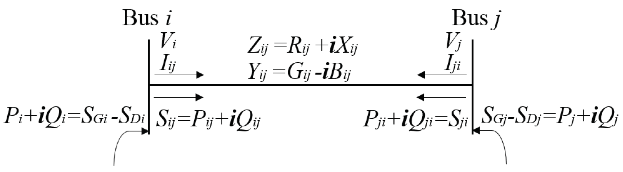
For each bus node $i\in N^0$, the variables are in capital letters, and the subscripts of them represent the bus node numbers. $U_i$ denotes the voltage in node i, $I_i$ denotes the injection current of node i. We define $P_{Gi}$ and $P_{Di}$ for a node i, where $P_{Di}$ denotes the active power of node i demanded, $P_{Gi}$ denotes the active power which node i generated. Similarly, we define $Q_{Gi}$ and $Q_{Di}$ the generated and demanded reactive power of node i. For the injection power of each node $S_i=(P_{Gi}-P_{Di})+\mathit{i}(Q_{Gi}-Q_{Di})$ denotes the complex power of node i, and $Y_i=G_i-\mathit{i}{B}_i$ denotes the admittance to ground.

For each line $(i,j)\in E$, let $I_{ij}$ denote the current from i to j and $I_{ijmax}$ denote the maximum transferred current of each line. Let $S_{ij}=P_{ij}+\mathit{i}{Q}_{ij}$ denote the transmission power from i to j, and $S_{ji}=P_{ji}+\mathit{i}{Q}_{ji}$ denote the transmission power from j to i. $Y_{ij}=G_{ij}-\mathit{i}{B}_{ij}$ denotes the admittance of the line. $Z_{ij}=R_{ij}+\mathit{i}{X}_{ij}$ denotes the line impedance and $Y_{ij}=\frac{1}{Z_{ij}}$. In the AC network, $U,Y,Z,I,S$ are all complex variables, $P,Q,G,B,R,X$ are all real variables.

Some notations are illustrated in Figure 1.

2.2. Optimal Power Flow Problem and Assumptions

An OPF problem can be stated mathematically as

$$\begin{array}{cc}\hfill \mathrm{Minimize}& f\left(x\right)\hfill \\ \hfill \mathrm{s}.\mathrm{t}.& g\left(x\right)=0\hfill \\ \hfill & h\left(x\right)\le 0.\hfill \end{array}$$

(1)

This is an optimization format where the objective function is described as $f\left(x\right)$ here and $g\left(x\right)$ represents all the equality constraints of the variable x. $h\left(x\right)$ means the inequality constraints. The word “s.t.” is the abbreviation of the phrase “subject to”. As summarized in Equation (1), we make the problems by minimizing the value of $f\left(x\right)$ when the equality constraints $g\left(x\right)$ and inequality constraints $h\left(x\right)$ are satisfied and x is the optimization variable.

2.2.1. Objective Functions

The objective function $f\left(x\right)$ in OPF generally focuses on the transmission power losses or total generators’ costs. The power loss can be formulated with the square of transmission current or the square voltage of bus nodes. The generators’ cost function can be described with the non-negative thermal plants’ coefficients $c_i$ and the generators’ active power $P_G$. It can be shown as

$$f(I_{ij},P_{Gi})=\sum _{(i,j)\in E}{I}_{ij}^2{R}_{ij}+\sum _{i\in G}{c}_i{P}_{Gi},$$

(2)

The total power loss is represented with $\sum I_{ij}^2{R}_{ij}$ here. $\sum c_i{P}_{Gi}$ is the total generators’ cost. In this paper, our objective functions involve a new term of current margin considering the thermal stability limit.

In a power system, there is always a specific limit for the apparent power or current that can be transferred from one node to another. This constraint only considers the maximum transforming limit rather than margins of the branch. For a specific line, the percentage of transmission current and limit current constructs the current margins. Let ${\phi }_{ij}=\frac{I_{ij}}{I_{ijmax}}$ be an index variable where $I_{ijmax}$ represents the maximum transferred current of each line $(i,j)$ which is greater than 0. If each of branch is labeled with $i_k{j}_k$ where in radial network k ranges from 1 to n, there is ${\phi }_{i_1{j}_1},{\phi }_{i_2{j}_2},\cdots ,{\phi }_{i_n{j}_n}$ individually for every line where $(i_1,j_1),(i_2,j_2),\cdots ,(i_n,j_n)\in E$. With a relative small and similar value on ${\phi }_{i_k{j}_k}$, enough current margins will be acquired on all lines. For the connected lines, it goes as follows:

$$0<{\phi }_{i_1{j}_1}={\phi }_{i_2{j}_2}=\cdots ={\phi }_{i_n{j}_n}<1$$

(3)

To simplify the notations, ${\phi }_{i_k{j}_k}$ will be abbreviated to $\phi$. To obtain the uniform current margins, (3) should be added as a constraint in OPF. However, this cannot be strictly satisfied considering different situations of operation. Our targets are to get the relatively similar current margins which means to approach (3) instead of exactly being at (3). We prefer small difference in $\phi$ of neighboring branches. Due to the Cauchy-Buniakowsky-Schwarz inequality theorem [27], it is known (3) can be obtained when the lower bound of $\sum {\phi }^2$ is acquired under the condition that the sum of $\phi$ is fixed, and $0<\phi <1$. Therefore, we put the $\sum {\phi }^2$ in the objective functions. The objective functions considering current margins will be shown as:

$$f(I_{ij},P_{Gi})=\kappa \sum _{(i,j)\in E}{I}_{ij}^2{R}_{ij}+\beta \sum _{i\in G}{c}_i{P}_{Gi}+\iota \sum _{(i,j)\in E}\frac{I_{ij}^2}{I_{ijmax}^2},$$

(4)

where $\beta ,\kappa ,\iota$ are the weight coefficients here.

2.2.2. Equality Constraints

The equality constraints $g\left(x\right)$ in OPF are about load flow equations which are governed by the Kirchhoff’s law and power balance’s law. For two bus nodes i and j in a connected branch as shown in Figure 1, the formulation goes as follows:

$$\begin{array}{c}{S}_{ij}=U_i{I}_{ij}^H,\hfill \end{array}$$

(5a)

$$\begin{array}{c}{I}_{ij}=(U_i-U_j)Y_{ij},\hfill \end{array}$$

(5b)

$$\begin{array}{c}\mathsf{\Sigma }{S}_{ij}=(P_{Gi}-P_{Di})+\mathit{i}(Q_{Gi}-Q_{Di}).\hfill \end{array}$$

(5c)

Equation (5) shows the load flow equations of each line. Equation (5a) demonstrates the relations of the node voltage, transmission current and complex power. The Equation (5b) describes the relationship of transmission current and voltage difference. Equation (5c) means each node’s power is governed by the power balance law.

2.2.3. Inequality Constraints

The inequality constraints $h\left(x\right)$ refer to limit of transmission power and current, limits for voltage and capacity power considering system’s stable and safe operation. Let $P_{Gimin}$, $P_{Dimin}$ and $P_{Gimax}$, $P_{Dimax}$ denote lower and upper bounds of the generated and demanded active power, $Q_{Gimin}$, $Q_{Dimin}$ and $Q_{Gimax}$, $Q_{Dimax}$ denote lower and upper bounds of the generated and demanded reactive power. For a load node, the bounded values of $P_{Gi}$ and $Q_{Gi}$ are regulated 0. For the non-dispatchable load, the value of $P_{Dimin}$ and $P_{Dimax}$, $Q_{Dimin}$ and $Q_{Dimax}$ will remain the same as its demand value respectively. Then $P_{Gi},P_{Di},Q_{Gi},Q_{Di}$ can be constrained as:

$$\begin{array}{c}{P}_{Gimin}\le P_{Gi}\le P_{Gimax},\hfill \end{array}$$

(6a)

$$\begin{array}{c}{Q}_{Gimin}\le Q_{Gi}\le Q_{Gimax},\hfill \end{array}$$

(6b)

$$\begin{array}{c}{P}_{Dimin}\le P_{Di}\le P_{Dimax},\hfill \end{array}$$

(6c)

$$\begin{array}{c}{Q}_{Dimin}\le Q_{Di}\le Q_{Dimax}.\hfill \end{array}$$

(6d)

In the power system, the voltage of each node should not fluctuate much from the sending point to the receiving point. The limits are usually $\pm 5\%$ within the base voltage value. $U_{imin}$ and $U_{imax}$ represents the minimum and maximum voltage value respectively. $U_i$ gets the following constraints:

$$\begin{array}{c}\hfill U_{imin}\le U_i\le U_{imax}.\end{array}$$

(7)

The nodes following Equation (7) are the ones that do not connect to the main grid, that is to say $i\in N$. While for the slack bus which connects to the grid, the power limits of active power and reactive power can vary from $-\infty$ to ∞. However, we always regulate its voltage to be $1+0i$ under unitary or regulate with a fixed voltage $U_0^{ref}$.

For a transmission line from i to j, there are some constraints for the thermal limit to make sure that the transmission line operates safely and stably. It can be shown as follows:

$$|I_{ij}|\le I_{ijmax}$$

(8)

where $I_{ijmax}$ denotes the maximum limit of the transmission current. Usually, it depends on the transmission line’s length and materials. We may use (8) for each line separately in different occasions.

2.2.4. OPF Problem and Assumptions

The OPF problem can be represented according to the above formulations:

$$\begin{array}{cc}\hfill \mathrm{Minimize}& \left(4\right)\hfill \\ \hfill \mathrm{s}.\mathrm{t}.& \left(5\right),\left(6\right),\left(7\right),\left(8\right)\hfill \end{array}$$

(9)

In this paper, we make the following assumptions:

• The network graph $\mathcal{G}$ in network topology is connected.
• The OPF in (9) is feasible.

3. OPF in Conic Format

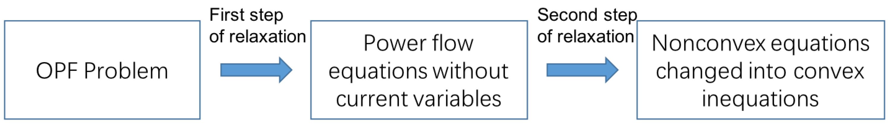
Due to the nonlinear equality constraints in (5a), OPF is a nonlinear and nonconvex program problem which is hard to find the global optimal solution. To make OPF solvable in polynomial time and the optimal operation point found, we change OPF problem into a convex optimization format. In this part, we aim to solve OPF problem (9) through two steps of relaxations. After the fist step, the current variables in OPF problem will be wade away. In the second step, the quadric equations will be relaxed with SOCP relaxations. The OPF problem can be solved thus by convex optimizations and the global optimum can be obtained successfully. The structure of this section is summarized in Figure 2.

3.1. First Step

The first step of relaxation is to handle with the current variables. By eliminating the current variables, the non-convexitiy in power flow constraints (5a) will be changed. In the transformation, we introduce the variables $S_{ij}$ and $S_{ji}$ at the same time for a transmission line $i,j$. $S_{ij}$ denotes the direction of current form i to j and $S_{ji}$ denotes the power transformed form j to i. Please note that on the transmission line $i\sim j$, the current from i to j equals to the value of $-I_{ji}$. However, due to the voltage difference, the transmission power $S_{ij}$ does not equal to $-S_{ji}$. By eliminating the variables $I_{ij}$ and $I_{ji}$, the power flow formulation becomes:

$$\begin{array}{cc}\hfill \mathsf{\Sigma }{S}_{ij}& =(P_{Gi}-P_{Di})+\mathit{i}(Q_{Gi}-Q_{Di}),\hfill \end{array}$$

(10a)

$$\begin{array}{cc}\hfill S_{ij}& =Y_{ij}^H{U}_i{U}_i^H-Y_{ij}^H{U}_i{U}_j^H,\hfill \end{array}$$

(10b)

$$\begin{array}{cc}\hfill S_{ji}& =Y_{ij}^H{U}_j{U}_j^H-Y_{ij}^H{U}_j{U}_i^H.\hfill \end{array}$$

(10c)

We define the variables as:

$$\begin{array}{cc}{V}_i=U_i{U}_i^H,\hfill & i\in N\hfill \\ V_{ij}=U_i{U}_j^H.\hfill & (i,j)\in E\hfill \end{array}$$

(11)

where $V_i\in \mathbb{R}$ and $V_i\ge 0,V_{ij}\in \mathbb{C}$. Through the transformation, the following power flow formula can be obtained by substituting variables:

$$\begin{array}{cc}\hfill \mathsf{\Sigma }{S}_{ij}& =(P_{Gi}-P_{Di})+\mathit{i}(Q_{Gi}-Q_{Di}),\hfill \end{array}$$

(12a)

$$\begin{array}{cc}\hfill S_{ij}& =Y_{ij}^H{V}_i-Y_{ij}^H{V}_{ij},\hfill \end{array}$$

(12b)

$$\begin{array}{cc}\hfill S_{ji}& =Y_{ij}^H{V}_j-Y_{ij}^H{V}_{ij}^H,\hfill \end{array}$$

(12c)

where $i\in N,i,j\in E$.

With the transformation, there is relationship for the voltage of each line. It can be shown as:

$$|V_{ij}{|}^2=V_i{V}_j.$$

(13)

Equation (12) together with (13) is the new power flow constraints that indicate the current, voltage and power balance in each branch of a power system topology. It is the power flow constraints instead of the (5).

From Equation (12) above, we can see that $V_{ij}$ and $V_{ij}^H$ exist at the same time. For a convex optimization problem, all the equality constraints should be affine, the objective functions and inequality constraints should be convex functions. The Equation (12b) combining with (12c) together are no longer affine functions due to the non-affine relationship between $V_{ij}$ and $V_{ij}^H$. Therefore we change the power flow constraints in the real number filed and replace $V_{ij}$ and $V_{ij}^H$ with new variables in real number field.

Below we decouple the active and reactive power, real and imaginary parts of voltage and current totally; the complex problem is changed into a real convex problem. More details about convex optimization can be seen in [28]. The active and reactive power balance equation can be described as

$$\begin{array}{cc}\hfill P_{Gi}-P_{Di}& =\mathsf{\Sigma }{P}_{ij},\hfill \end{array}$$

(14a)

$$\begin{array}{cc}\hfill Q_{Gi}-Q_{Di}& =\mathsf{\Sigma }{Q}_{ij},\hfill \end{array}$$

(14b)

where $i\in N$ and $(i,j)\in E$. $P_{Gi}$ and $P_{Di}$ are always equal or larger than zero. The equations above means the total power of node i is the sum power of all connecting branches. The real and imaginary part of $V_{ij}$ is defined as $a_{ij}$ and $b_{ij}$. That is to say,

$$V_{ij}=a_{ij}+b_{ij}\mathit{i}.$$

(15)

Then the relations of $P_{ij}$,$P_{ji}$,$Q_{ij}$,$Q_{ji}$ can be shown as follows:

$$\begin{array}{c}{P}_{ij}=G_{ij}(V_i-a_{ij})+B_{ij}{b}_{ij},\hfill \end{array}$$

(16a)

$$\begin{array}{c}{P}_{ji}=G_{ij}(V_j-a_{ij})-B_{ij}{b}_{ij},\hfill \end{array}$$

(16b)

$$\begin{array}{c}{Q}_{ij}=-G_{ij}{b}_{ij}+B_{ij}(V_i-a_{ij}),\hfill \end{array}$$

(16c)

$$\begin{array}{c}{Q}_{ji}=G_{ij}{b}_{ij}+B_{ij}(V_j-a_{ij}).\hfill \end{array}$$

(16d)

The Equation (13) can be represented as

$$a_{ij}^2+b_{ij}^2=V_i{V}_j,$$

(17)

because of (15).

Since there are no more variables as $I_{ij}$ in the power flow constraints, the objective functions should be reformulated correspondingly.

For (4), the power loss of $i\sim j$ can be represented with the sum of $P_{ij}$ and $P_{ji}$. The active power loss is consumed by the resistance of the line. For ${\phi }^2$ here, we can describe as

$${\phi }_{ij}^2=\frac{(P_{ij}+P_{ji})}{R_{ij}{I}_{ijmax}^2}(i,j)\in E$$

The objective function (4) can be shown as:

$$g(P_{ij},P_{ji},P_{Gi})=\sum _{(i,j)\in E}{\alpha }_{ij}[P_{ij}+P_{ji}]+\beta \sum _{i\in G}f\left(P_{Gi}\right),$$

(18)

where

$${\alpha }_{ij}=\kappa +\frac{\iota }{R_{ij}{I}_{ijmax}^2}.$$

(19)

The objective function is concerned with the active power of each line which can be written as:

$$\begin{array}{c}\hfill \mathrm{Minimize}g\left(P\right),\end{array}$$

(20)

where P refers to $(P_{ij},P_{ji},P_{Gi})$. It should be noted the objective functions here can get the same value of (4). For the voltage constraint, it will be for the new variables $V_i$ instead of $U_i$.

$$\begin{array}{c}{U}_{min}^2\le V_i\le U_{max}^2,i\in N\hfill \\ V_0=U_{ref}^2.\hfill \end{array}$$

(21)

$U_{ref}$ denotes the reference voltage of the slack node.

For the inequality constraints (8), the constraints for $I_{ij}$ can be represented with the variables $P_{ij}$ since $P_{ij}=I_{ij}^2{R}_{ij}$ and $R_{ij}$ is a constant variable. For the line $i\sim j$, the maximum transmission value of $I_{ij}$ is same as that of $-I_{ji}$, which both represents the current limit of the line $(i,j)$. The constraints (8) can be represented as:

$$\begin{array}{c}\hfill -R_{ij}{I}_{ijmax}^2\le P_{ij}\le R_{ij}{I}_{ijmax}^2,\\ \hfill -R_{ij}{I}_{ijmax}^2\le P_{ji}\le R_{ij}{I}_{ijmax}^2.\end{array}$$

(22)

With the variables $P_{ij}$ and $P_{ji}$, we have the following constraints considering the actual physical meanings.

$$P_{ij}+P_{ji}\ge 0.$$

(23)

When the value of $I_{ij}$ is positive, the value of $I_{ji}$ must be negtive and vice versa. The sum of $P_{ij}$ and $P_{ji}$ represents the power loss of the transmission line which should be positive.

After the first step of relaxation, the relaxed OPF problem is like this:

$$\begin{array}{cc}\hfill \mathrm{Minimize}& g\left(P\right)\hfill \\ \hfill \mathrm{s}.\mathrm{t}.& \left(14\right),\left(16\right),\left(17\right),\left(6\right),\left(21\right),\left(22\right),\left(23\right)\hfill \end{array}$$

(24)

The objective functions $g\left(P\right)$ in a convex function of variables. The equality constraints (14a)–(14b) and (16a)–(16d) are totally linear and affine and in a simple form. The equality constraints (17) are in quadratic form. The inequality constraints (6), (21), (22) and (23) are all convex. Besides all the variables are in real format. To make this problem a convex optimization, we need to do with the non-affine equality constraints (17). This will be done in the next step.

3.2. Second Step

SOCP relaxations are applied to quadratic equations to convexify the OPF problem in this subsection.

The quadric Equation (17) is converted into an inequality constraint after the relaxation. The quadratic equation is changed into a rotating cone when relaxing the sign of equality into the sign of inequality.

$$a_{ij}^2+b_{ij}^2\le V_i{V}_j.$$

(25)

This Equation (25) can be presented as a cone in a 2-norm form.

$${∥\begin{array}{c}2a_{ij}\\ 2b_{ij}\\ V_i-V_j\end{array}∥}_2\le V_i+V_j.$$

(26)

This way, the inequality constraints are in conic format. The OPF (24) becomes a convex optimization problem in real field after the second step of relaxation:

$$\begin{array}{cc}\hfill \mathrm{Minimize}& g\left(P\right)\hfill \\ \hfill \mathrm{s}.\mathrm{t}.& \left(14\right),\left(16\right),\left(25\right),\left(6\right),\left(21\right),\left(22\right),\left(23\right).\hfill \end{array}$$

(27)

To guarantee the correctness of the solution, it is expected that the final result exists on the bound of the cone. If we get the solution when the formulation (26) acquires the equal sign, the relaxation is what we call it an exact relaxation. When (26) gets the exact relaxations, the relaxed problem is equal to (24) then. The exactness of the relaxation will be illustrated in the next section.

3.3. Relaxation Discussions

It is (27) that is the final presenting form in this paper. It is in a standard convex optimization format, which ensures global optimality. The objective function considering power loss and current margins here are linear independent with variables $P_{ij}$ and $P_{ji}$. In addition, the generators’ cost objective is a convex function with variables $P_{Gi}$. Therefore, it is regarded as a convex objective function in OPF problem. The nonconvexity in the power flow constraints changes into convex constraints after two steps of relaxations. Then, all the variables above are in $\mathbb{R}$, the equality constraints are in affine format, and the inequality constraints are convex functions. From the formulation, we can know that the optimization problem is about variables $P_{Gi},P_{Di},Q_{Gi},Q_{Di},V_i,a_{ij},b_{ij}$ and $P_{ij},P_{ji},Q_{ij},Q_{ji}$ are the intermediate variables.

Compared with the SDP relaxation method mentioned in [20], we transform the positive semidefinite matrix of the voltage into some $2X2$ ones, the number of which depend on branches’ amount. We improve the operational efficiency this way. Furthermore, with the bus injection model adding branch variables, we make the current margin as a part of objective functions under thermal stability consideration. The optimal solution of this objective function will leave enough margins to branches and contribute to the power system’s stable operation. Compared with the SOCP relaxation method proposed in the branch flow model in [21], we do not use the current variables in the model. Instead, we use voltage variables. In addition, for each branch, we focus on the branch itself. In branch flow OPF, when building up model for node i, it regulates the direction of transmission such as $k\sim i$ and $i\sim j$. In the above method, we split the power system with nodes and there is no need to regulate the transforming direction for the branches.

The OPF solutions of voltage U can be recovered from square root calculations of $V_i$ and division operations of $a_{ij}+b_{ij}\mathit{i}$. With the solutions of $V_i,a_{ij},b_{ij}$, we present the following Algorithm 1 to recover voltage of each node. In this algorithm, we first make the value of $U_0$ equal to $U_0^{ref}$ and initialize the set $M_{stay}$ with number 0. When the set $M_{stay}$ is not equal to the set $N^0$, the algorithm runs into the loop. In this loop, we will get the voltage value of the node and update the $M_{stay}$ at the same time. When the set $M_{stay}$ is same as the set $N^0$, the loop will end.

Algorithm 1: Recover U from $V_i$, $a_{ij}$ and $b_{ij}$

Input:($V_i,a_{ij},b_{ij}$) that satisfies Lemma 1

Output:U

1. $U_0$←$U_0^{ref}$;

2. $M_{stay}$← 0;

3. while $M_{stay}\ne N^0$ do

find $i\to j$ that $i\in M_{stay}$ and $j\notin M_{stay}$;

compute $U_j\to \frac{a_{ij}-bij\mathit{i}}{U_i^H}$;

$M_{stay}\to M_{stay}\cup$j;

end while

Lemma 1.

Let$V_i\in \mathbb{R}$for$i\in N^0$, let$a_{ij}$and$b_{ij}$ for $(i,j)\in E$.

If 1.$V_0=U_0^{ref}{\left[U_0^{ref}\right]}^H$for$U_0^{ref}\in \mathbb{C}$;

 2. $V_i$ is nonzero for $i\in N^0$;

 3. $V_i{V}_j=a_{ij}^2+b_{ij}^2$;

then the above algorithm computes the unique$U_i$that satisfies

$$\begin{array}{c}{U}_0=U_0^{ref}\hfill \end{array}$$

(28a)

$$\begin{array}{c}{V}_i=\left(U_i\right){\left(U_i\right)}^{H}i\in N,\hfill \end{array}$$

(28b)

$$\begin{array}{c}{a}_{ij}+b_{ij}\mathit{i}=U_i{U}_j^H(i,j)\in E.\hfill \end{array}$$

(28c)

Proof of Lemma 1.

We will proof this with the recursive algorithm. The total recursive time is denoted by the postive interger T. Let t indicate the recursive time where $t=1,2,\cdots ,T$. Let $M_{\left(0\right)}=0$, $M_t$ represent the set $M_{stay}$ after the t recursion.

In the algorithm, for node 0 we simplify name one of the nodes connecting to it with number 1. When $t=0$, it is easy to know:

$$\begin{array}{c}{V}_0=\left(U_0\right){\left(U_0\right)}^H,\hfill \end{array}$$

(29a)

$$\begin{array}{c}{V}_1\ne 0,\hfill \end{array}$$

(29b)

$$\begin{array}{c}{a}_{01}^2+b_{01}^2=V_0{V}_1.\hfill \end{array}$$

(29c)

Because of Algorithm 1, it can be obtained:

$$\begin{array}{c}{U}_0=U_0^{ref}\hfill \end{array}$$

(30a)

$$\begin{array}{c}{a}_{01}-b_{01}\mathit{i}=U_1{U}_0^H.\hfill \end{array}$$

(30b)

It satisfies (28a) naturally due to (30a). Combining (29) and (30b) together, we will get the following equations:

$$\begin{array}{c}{a}_{01}+b_{01}\mathit{i}=U_0{U}_1^H,\hfill \end{array}$$

(31a)

$$\begin{array}{c}{V}_1=U_1{U}_1^H.\hfill \end{array}$$

(31b)

It satisfies (28b) and (28c) at the same time. Therefore, Lemma 1 is satisfied for node 0 and the branch connecting to node 0. Assume Lemma 1 holds for the node k and the branch $(k-1,k)$ after the t recursion where $k-1\in M_t,k\in M_t,1<t<T-1$. Therefore for one of the nodes connecting to k which is denoted as $k_1$ and $k_1\notin M_t$, we can know:

$$\begin{array}{c}{V}_k=U_k{U}_k^H,\hfill \end{array}$$

(32a)

$$\begin{array}{c}{V}_{k_1}\ne 0,\hfill \end{array}$$

(32b)

$$\begin{array}{c}{a}_{k,k_1}^2+b_{k,k_1}^2=V_k{V}_{k_1}.\hfill \end{array}$$

(32c)

Similarly, applying Algorithm 1 in the $t+1$ recursion, we can get:

$$\begin{array}{c}\hfill a_{k,k_1}-b_{k,k_1}\mathit{i}=U_{k_1}{U}_k^H.\end{array}$$

(33)

Combining (32) and (33), we can get

$$\begin{array}{c}{a}_{k,k_1}+b_{k,k_1}\mathit{i}=U_k{U}_{k_1}^H,\hfill \end{array}$$

(34a)

$$\begin{array}{c}{V}_{k_1}=U_{k_1}{U}_{k_1}^H.\hfill \end{array}$$

(34b)

(28) is satisfied for the node $k_1$ and the connecting branch $k\sim k_1$. Therefore, Lemma 1 holds for $t+1$ recursion. This completes the proof that Algorithm 1 computes a U that satisfies (28). □

Please note that such recursion holds on condition that the network topology is radial. In radial networks, introducing a new node will only lead to one new branch. While in mesh networks, a new node introduced will construct more than one branch when the node is in a circle. This makes it no more sufficient in the recursion.

Lemma 1 offers a way to recover the OPF solution of (9) from the solution of (27) under the condition that the second step of relaxation is exact.

For constraints, the solution of (27) with variables $P_{Gi},Q_{Gi},P_{Di},Q_{Di},a_{ij},b_{ij}$ satisfy the equality and inequality constraints in (27). The Algorithm 1’s recovered variables $P_{Gi},Q_{Gi},P_{Di},Q_{Di},U_i$ can be proved to satisfy the constraints (5)–(8) by putting (28) and (14), (16), (17), (6), (21), (22), (23) into the formula. This implies that when the second step of relaxation is exact, the relaxed OPF constraints can accord with primal OPF constraints equivalently.

For objective functions in (9) and (27), we can get some $f(I_{ij},P_{Gi})=g(P_{ij},P_{ji},P_{Gi})$ here. In the first step of relaxation above, we can see the first step is done by introducing variables $V_i,a_{ij}$ and $b_{ij}$ satisfying $V_i=U_i{U}_i^H$ and $U_i{U}_j^H=a_{ij}+b_{ij}\mathit{i}$. With each $I_{ij}$ and $U_i$, we can get the corresponding $V_i,a_{ij}$, $b_{ij},P_{ij}$ and $P_{ji}$. Thus,

$$f(I_{ij},P_{Gi})\le g(P_{ij},P_{ji},P_{Gi}).$$

(35)

Due to Lemma 1, with Algorithm 1 we can recover $U_i$ and $I_{ij}$. Subsequently,

$$g(P_{ij},P_{ji},P_{Gi})\ge f(I_{ij},P_{Gi}).$$

(36)

Then,

$$f(I_{ij},P_{Gi})=g(P_{ij},P_{ji},P_{Gi}).$$

(37)

Since solving (27) gets a global optimal solution of $g(P_{ij},P_{ji},P_{Gi})$, the recovered solution will be the global optimum of $f(I_{ij},P_{Gi})$. Therefore, the recovered solution of relaxed OPF in Algorithm 1 is the optimal solution of OPF problem.

4. Exactness of the Relaxation

As is shown before, we call the relaxation is exact if the optimal solution is where the formulation (26) gets the equality sign. In this section, we will give one theorem to guarantee the exactness of relaxation.

Theorem 1.

If there is no upper bound on$P_{Dmax}$and$Q_{Dmax}$, the relaxation is exact then.

Proof of Theorem 1.

Assume we get a group of optimal solutions, $a_{ij},b_{ij},V_i$ and $V_j$. In addition, we get exact solutions on line $i\sim j$ where $i,j\ne 0$ except the particular line $k\sim l$. That is to say, $\{i,j\}\cap \{k,l\}\ne \varnothing$ and

$$\begin{array}{c}\hfill a_{ij}^2+b_{ij}^2=V_i{V}_{j}when\{i,j\}\ne \{k,l\},\\ \hfill a_{ij}^2+b_{ij}^2<V_i{V}_{j}when\{i,j\}=\{k,l\}.\end{array}$$

(38)

On the line $k\sim l$, we define

$$\begin{array}{cc}\hfill a_{kl}^{\ast }& =\sqrt{V_k{V}_l-b_{kl}},\hfill \\ \hfill b_{kl}^{\ast }& =b_{kl},\hfill \\ \hfill V_k^{\ast }& =V_k,\hfill \\ \hfill V_l^{\ast }& =V_l.\hfill \end{array}$$

(39)

We define the following variables with $a_{kl}^{\ast },b_{kl}^{\ast },V_k^{\ast },V_l^{\ast }$,

$$\begin{array}{cc}\hfill P_{kl}^{\ast }& =G_{kl}(V_k^{\ast }-a_{kl}^{\ast })+B_{kl}{b}_{kl}^{\ast },\hfill \\ \hfill P_{lk}^{\ast }& =G_{kl}(V_l^{\ast }-a_{kl}^{\ast })-B_{kl}{b}_{kl}^{\ast },\hfill \\ \hfill Q_{kl}^{\ast }& =-G_{kl}{b}_{kl}^{\ast }+B_{kl}(V_k^{\ast }-a_{kl}^{\ast }),\hfill \\ \hfill Q_{lk}^{\ast }& =G_{kl}{b}_{kl}^{\ast }+B_{kl}(V_l^{\ast }-a_{kl}^{\ast }).\hfill \end{array}$$

(40)

Since $a_{kl}^2+b_{kl}^2<V_k{V}_l$, $a_{kl}^{\ast }$ is larger than $a_{kl}$. Then

$$P_{kl}^{\ast }-P_{kl}=G_{kl}(V_k^{\ast }-a_{kl}^{\ast })+B_{kl}{b}_{kl}^{\ast }-G_{kl}(V_k-a_{kl})-B_{kl}{b}_{kl}=G_{kl}(a_{kl}^{\ast }-a_{kl})<0,$$

(41)

$$Q_{kl}^{\ast }-Q_{kl}=-G_{kl}{b}_{kl}^{\ast }+B_{kl}(V_k^{\ast }-a_{kl}^{\ast })+G_{kl}{b}_{kl}-B_{kl}(V_k-a_{kl})=B_{kl}(a_{kl}^{\ast }-a_{kl})<0.$$

(42)

The Equations (41) and (42) represent the difference of the transmission power on branch $k\sim l$. For the injected active power at node k and l, we can get

$$\begin{array}{cc}\hfill P_{Gk}^{\ast }-P_{Dk}^{\ast }& =P_{kl}^{\ast }+{\mathsf{\Sigma }}_{k\ast \sim i}{P}_{ki}^{\ast }\hfill \\ & =P_{kl}^{\ast }+{\mathsf{\Sigma }}_{k\ast \sim i}{P}_{ki}<P_{Gk}-P_{Dk}\hfill \\ \hfill P_{Gl}^{\ast }-P_{Dl}^{\ast }& =P_{lk}^{\ast }+{\mathsf{\Sigma }}_{l\ast \sim i}{P}_{li}^{\ast }\hfill \\ & =P_{lk}^{\ast }+{\mathsf{\Sigma }}_{l\ast \sim i}{P}_{ki}<P_{Gl}-P_{Dl}\hfill \\ \hfill Q_{Gk}^{\ast }-Q_{Dk}^{\ast }& =Q_{kl}^{\ast }+{\mathsf{\Sigma }}_{k\ast \sim i}{Q}_{ki}^{\ast }\hfill \\ & =Q_{kl}^{\ast }+{\mathsf{\Sigma }}_{k\ast \sim i}{Q}_{ki}<Q_{Gk}-Q_{Dk}\hfill \\ \hfill Q_{Gl}^{\ast }-Q_{Dl}^{\ast }& =Q_{lk}^{\ast }+{\mathsf{\Sigma }}_{l\ast \sim i}{Q}_{li}^{\ast }\hfill \\ & =Q_{lk}^{\ast }+{\mathsf{\Sigma }}_{l\ast \sim i}{Q}_{ki}<Q_{Gl}-Q_{Dl}\hfill \end{array}$$

(43)

When the demanded active power at node k and l remains unchanged, $P_{Gk}^{\ast }<P_{Dk}$ and $P_{Gl}^{\ast }<P_{Dl}$. When the demanded reactive power at node k and l remains unchanged, $Q_{Gk}^{\ast }<Q_{Dk}$ and $Q_{Gl}^{\ast }<Q_{Dl}$. If the value of $P_G$ and $Q_G$ has already reached the lower bound of $P_{Gmin}$ and $Q_{Gmin}$, we can change the value of $P_{Di}$ and $Q_{Di}$ due to the fact there is no upper bound for $P_{Dmax}$ and $Q_{Dmax}$. The value of $P_{Gi}$ and $Q_{Gi}$ will remain unchanged then which will satisfy the constraint (6). According to the objective functions of power cost are strictly increasing in variables $P_G$, the objective function with the variable $P_G$ will have a smaller value or the same value. Besides,

$$\begin{array}{c}\hfill P_{kl}^{\ast }+P_{lk}^{\ast }-(P_{kl}+P_{lk})=G_{kl}(V_k^{\ast }-V_k+V_l^{\ast }-V_l-2a_{kl}^{\ast }+2a_{kl})<0.\end{array}$$

(44)

Then, the objective function with $P_{ij}+P_{ji}$ has a smaller value.

For this set of solutions $a_{kl}^{\ast },b_{kl}^{\ast },V_k^{\ast },V_l^{\ast }$, we can know that this satisfies (14) and (16) according to (40) and (43). Obviously, this set of solution satisfies (25), (6), (21), (22),(23). Therefore, the solutions satisfy the constraint (14) and (6). In addition, it is definitely a solution of (24) and has a better value on objective functions. The optimal solution is such that every inequality sign in Equation (26) achieves equality sign. This concludes the proof. □

Please note that there is no upper bound on the active and reactive demand power means for a node i, we can supply more power than it originally needed, this can be called load over-satisfaction condition. This condition has been mentioned in ref. [20] and ref. [21]. From the proof above, we can know that if the relaxation is not exact, we can always find a better optimal solution which contradicts the global optimum. Therefore, we can get the exact solutions under this over satisfaction condition. Besides, the proof has no relation with the network structure. This works for the mesh network as well.

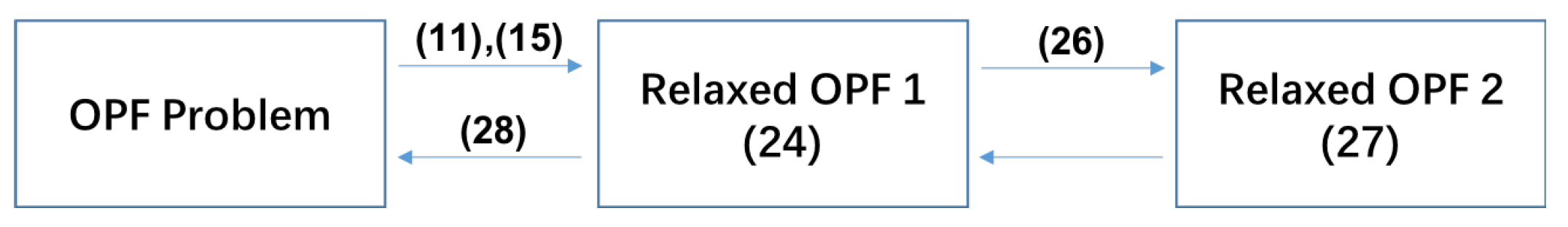
From all above, the proposed two step relaxation can be summarized by the following Figure 3.

5. Case Study

The novel OPF formulation is tested in some cases in this section. One is a six-node system as an example and the other is the standard IEEE benchmark systems which helps to verify whether the relaxations are exact. The case studies are evaluated on a computer whose CPU is Intel Core 5 at 2.9 GHz with 8 G RAM. The operation system is Mac OS 10.13. The YALMIP [29] is used to depict the variables of the model in Matlab 2016a. In addition, the CPLEX [30] solver is used to solve the convex relaxation problems.

5.1. A 6-Node Small System Example

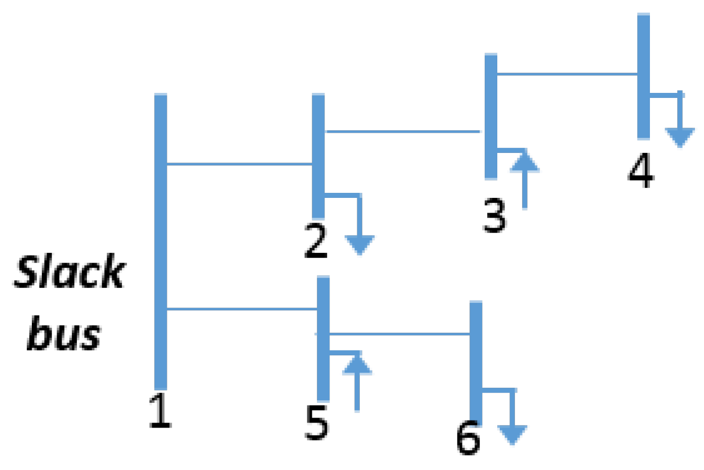
In the simple radial network, there are six nodes and five branches in total as shown in Figure 4. In this system, the node 1 refers to the default slack bus. The node 3 and 5 represent the generator node, and the node 2, 4 and 6 is the adjustable load nodes with controllers. The specific parameters are summarized in the below

Table 1. 6-Node System Bus Parameters.

Bus Parameters
Node	P	Q	Vmin	Vmax	${\mathit{c}}_{\mathbf{0}}$	${\mathit{c}}_{\mathbf{1}}$	${\mathit{c}}_{\mathbf{2}}$
1	∞	∞	1	1	0.22	2.5	0.11
2	−2.4	−3.2	0.8	1.2	0	0	0
3	limit	limit	0.8	1.2	0.25	2.4	0.85
4	−3.5	−1.8	0.8	1.2	0	0	0
5	limit	limit	0.8	1.2	0	2.4	0.25
6	−2.5	0	0.8	1.2	0	0	0

and

Table 2. 6-Node System Line Parameters.

Line Parameters
From to Node	r	x	b	${\mathit{p}}_{\mathit{lim}}$	${\mathit{q}}_{\mathit{lim}}$
1–2	0.05	0.20	0.030	7.5	4.5
1–5	0.10	0.20	0.040	7.5	4.5
2–3	0.05	0.075	0.070	7.5	4.5
3–4	0.01	0.01	0.030	7.5	4.5
5–6	0.01	0.01	0.04	7.5	4.5

, and all the values are in per unit quantities (100MVA Base).

The OPF problems can be formulated with Equation (27). Therefore, each branch is constrained with 7 formulations, 3 of which are inequality constraints and 4 of which are equality equations. For the nodes, considered on the limit, two equality constraints and five inequality constraints are applied for each node.

Our optimization objective of this system is to minimize the total cost, transmission loss and to the best of uniform current margin of the system. We firstly make the objective function $g=P_{ij}+P_{ji}+f\left(P_{Gi}\right)$ focusing on transmission loss and power cost and denote it as LC. Moreover, we choose objective function as $g=(1+\frac{1}{R_{ij}{I}_{ijmax}^2})(P_{ij}+P_{ji})+f\left(P_{Gi}\right)$ and denote it as LCC. In these two models, the weight coefficients are all equal to 1. Applying the data in Table 1 and Table 2, we get the corresponding result as follows in

Table 3. Branch value.

Objective Function	LC		LCC
Branch No.	${\mathit{P}}_{\mathit{ij}}+{\mathit{P}}_{\mathit{ji}}$	$\mathit{\phi }$	${\mathit{P}}_{\mathit{ij}}+{\mathit{P}}_{\mathit{ji}}$	$\mathit{\phi }$
1–2	0.047295	0.30	0.055648	0.47
2–3	0.7975	0.88	0.76391	0.82
3–4	0.11632	0.55	0.11632	0.55
1–5	0.0019792	0.38	0.02467	0.49
5–6	0.061718	0.95	0.071718	0.82
Total power loss	1.025		1.032

. The transmission loss of each branch here is denoted with $P_{ij}+P_{ji}$, and we calculate the value of $\phi$ in each branch. All the values are in per unit quantities (100MVA Base).

We list the corresponding bus value in

Table 4. Bus value.

Objective Function	LC		LCC
Bus No.	${\mathit{P}}_{\mathit{Gi}}$	$\mathit{V}$	${\mathit{P}}_{\mathit{Gi}}$	$\mathit{V}$
1	0.72371	1	0.9011	1
2	0	0.88	0	0.87
3	6.0817	0.94	5.8975	0.95
4	0	0.94	0	0.93
5	2.6266	1.2	2.6334	1.2
6	0	0.92	0	0.91
Total power cost	22.71		22.73

. The value of $P_{Gi}$ is the active power generated. In addition, V here is the square amplitude of node voltage.

Comparing the results above, we can see with current margin considered in OPF, there will be changes to the value of $\phi$ in each branch. As is shown in in Table 3, the $\phi$ of branch 2–3 and 5–6 are so large in LC. However, it becomes less somehow in LCC then. Similarly, the value of $\phi$ of branch 2–3 and 5–6 becomes larger in LCC than LC. In addition, at the cost of considering current margin, the active power generated will be more in LCC than LC as shown in Table 4. It can be seen the $\phi$ is not uniform when the weight coefficients equal to one. Further increasing the weight coefficients, we make the objective function as $F=(1+\frac{100}{R_{ij}{I}_{ijmax}^2})(P_{ij}+P_{ji})+f\left(P_{Gi}\right)$ and denote it as LCBC. This way we make the weight of current margin bigger than power loss and generators’ cost. We get the corresponding branch results as follows in

Table 5. Branch value of LCBC.

Branch No.	${\mathit{P}}_{\mathit{ij}}+{\mathit{P}}_{\mathit{ji}}$	$\mathit{\phi }$
1–2	0.068284	0.56
2–3	0.68128	0.60
3–4	0.11632	0.55
1–5	0.002786	0.54
5–6	0.046313	0.61

.

The corresponding bus value is listed in

Table 6. Bus value of LCBC.

Bus No.	${\mathit{P}}_{\mathit{Gi}}$	V
1	1.672	1
2	0	0.78
3	5.2342	1.1
4	0	0.97
5	2.6352	1.2
6	0	0.82

, where the value of $P_{Gi}$ is the generated active power and V is the square amplitude of node voltage.

From the results we can see different $\phi$ are in the tendency of accordance. The values of $\phi$ are around 0.5 then. With bigger weight of current margin objective, we obtain the relative uniform $\phi$.

5.2. Test Results in IEEE Benchmark

In the standard IEEE benchmark, the test networks are modified in the Matlab toolbox matpower. Since the IEEE systems are meshed, we split the circles of five systems for simulation. Our optimization objective function focuses on the active power loss, which is the sum of $P_{ij}$ and $P_{ji}$. The operation time is compared in two different models. The first model is proposed in [31] and we use the relaxed OPF 3 model metioned in the paper of which the SDP relaxations have been changed into SOCP ones. We denote this model as BIMR. The second model is according to (27) and denote this model as BIMBR. The comparison results are shown in

Table 7. Two Relaxation Tests in IEEE Benchmark Systems.

Relaxation	System	Power Loss	Operation Time
BIMR	IEEE 9	2.548	0.0262
	IEEE 14	13.574	0.0367
	IEEE 30	7.359	0.0486
	IEEE 57	19.482	0.0521
	IEEE 118	62.6212	0.1321
BIMBR	IEEE 9	2.548	0.0251
	IEEE 14	13.574	0.0334
	IEEE 30	7.359	0.0354
	IEEE 57	19.482	0.0425
	IEEE 118	62.6212	0.0905

. The unit of time is in second and all the values are in per unit quantities (100MVA Base)

It can be seen from Table 7 that the proposed relaxation makes OPF a convex and solvable optimization problem. The computation speed of the optimization is counted on the topology and scale of system. The optimal value of the objective functions is the same in two models. This shows that both of the relaxation is exact and tight. The model mentioned in [31] is in a complex number field and our model is illustrated in a real number filed, and as is shown in Table 7, the model proposed in this paper calculates faster than the bus injection model with SOCP relaxation of each branch, which is especially obvious in the large systems.

5.3. Discussions

From the case study above, it can be seen that this kind of method is applicable in both small networks and standard IEEE benchmark systems whose networks are transformed in radial formats. When the loads have not reached the maximum capacity, our relaxations can be proved to be exact. With our methods, the current margins of testing cases tend to be more uniform. Besides, compared with the relaxed SDP method, our method shows a better efficiency.

6. Conclusions

In this paper, we propose an OPF power flow formulation considering current margins in radial networks. With current margins in objective function, we obtain OPF solutions with relatively similar and enough margins of each branch. This OPF model makes it possible to consider the current margins under thermal stability consideration with new branch variables added to bus injection model. Applying the SOCP relaxations, the OPF is convex and solvable. With branch variables added into bus injection model, the proposed method is not sensitive to the system scale and has no need to define transmission directions. Moreover, we propose one sufficient condition to guarantee the exactness of relaxations. In the case studies, the simple 6-node network model shows relatively uniform current margins and the tests in standard IEEE benchmark systems using achieve a higher efficiency.

References

- Sakis, A.P.; Xia, F. Optimal Power Flow Application to Composite Power System Reliability Analysis. In Proceedings of the Joint International Power Conference Athens Power Tech, Athens, Greece, 5–8 September 1993; pp. 185–190. [Google Scholar]
- Carpentier, J. Contribution to the economic dispatch problem. Bull. Soc. Franc. Electr. 1962, 3, 836–845. [Google Scholar]
- Dommel, H.W.; Tinney, W.F. Optimal Power Flow Solutions. IEEE Trans. Power Appar. Syst. 1968, PAS-87, 1866–1876. [Google Scholar] [CrossRef]
- Shyamasundar, R.K. Introduction to Algorithms; MIT Press: Cambridge, MA, USA, 2010; pp. 14–24. [Google Scholar]
- Dvijotham, K.; Molzahn, D.K. Error bounds on the DC power flow approximation: A convex relaxation approach. In Proceedings of the 2016 IEEE 55th Conference on Decision and Control, Las Vegas, NV, USA, 12–14 December 2016; pp. 2411–2418. [Google Scholar]
- Stott, B.; Jardim, J.; Alsac, O. DC Power Flow Revisited. IEEE Trans. Power Syst. 2009, 24, 1290–1300. [Google Scholar] [CrossRef]
- Yang, Z.; Zhong, H.; Xia, Q.; Bose, A.; Kang, C. Optimal power flow based on successive linear approximation of power flow equations. IET Gener. Transm. Distrib. 2016, 10, 3654–3662. [Google Scholar] [CrossRef]
- Babu, M.R.; Harini, D. LP based solution for Security Constrained Optimal Power Flow. In Proceedings of the International Conference on Science Technology Engineering and Management, Chennai, India, 30–31 March 2016; pp. 355–359. [Google Scholar]
- Sasson, A.M.; Viloria, F.; Aboytes, F. Optimal Load Flow Solution Using the Hessian Matrix. IEEE Trans. Power Appar. Syst. 1973, PAS-92, 31–41. [Google Scholar] [CrossRef]
- Tinney, W.F.; Hart, C.E. Power Flow Solution by Newton’s Method. IEEE Trans. Power Appar. Syst. 2007, PAS-86, 1449–1460. [Google Scholar] [CrossRef]
- Li, X.; Sun, D.; Toh, K.C. An efficient linearly convergent semismooth Netwon-CG augmented Lagrangian method for Lasso problems. Siam J. Optim. 2016, 28, 433–458. [Google Scholar] [CrossRef]
- Raviprabakaran, V. Enhanced ant colony optimization to solve the optimal power flow with ecological emission. Int. J. Syst. Assur. Eng. Manag. 2016, 9, 58–65. [Google Scholar] [CrossRef]
- Li, M.S.; Tang, W.J.; Tang, W.H.; Wu, Q.H.; Saunders, J.R. Bacterial Foraging Algorithm with Varying Population for Optimal Power Flow. Biosystems 2010, 100, 185–197. [Google Scholar] [CrossRef] [PubMed]
- Sivasubramani, S.; Swarup, K.S. Sequential quadratic programming based differential evolution algorithm for optimal power flow problem. IET Gener. Transm. Distrib. 2011, 5, 1149–1154. [Google Scholar] [CrossRef]
- Radosavljević, J.; Jevtić, M.; Arsić, N.; Klimenta, D. Optimal power flow for distribution networks using gravitational search algorithm. Electr. Eng. 2014, 96, 335–345. [Google Scholar] [CrossRef]
- Kahourzade, S.; Mahmoudi, A.; Mokhlis, H.B. A comparative study of multi-objective optimal power flow based on particle swarm, evolutionary programming, and genetic algorithm. Electr. Eng. 2015, 97, 1–12. [Google Scholar] [CrossRef]
- King, R.T.F.A.; Tu, X.; Dessaint, L.A.; Kamwa, I. Multi-contingency transient stability-constrained optimal power flow using multilayer feedforward neural networks. In Proceedings of the Electrical and Computer Engineering, Vancouver, BC, Canada, 15–18 May 2016; pp. 1–6. [Google Scholar]
- Shilaja, C.; Ravi, K.; Shilaja, C.; Ravi, K. Optimal Power Flow Using Hybrid DA-APSO Algorithm in Renewable Energy Resources. Energy Procedia 2017, 117, 1085–1092. [Google Scholar] [CrossRef]
- Bai, X.; Wei, H.; Fujisawa, K.; Wang, Y. Semidefinite programming for optimal power flow problems. Int. J. Electr. Power Energy Syst. 2008, 30, 383–392. [Google Scholar] [CrossRef]
- Lavaei, J.; Low, S.H. Zero Duality Gap in Optimal Power Flow Problem. IEEE Trans. Power Syst. 2012, 27, 92–107. [Google Scholar] [CrossRef] [Green Version]
- Farivar, M.; Low, S.H. Branch flow model: Relaxations and convexification. In Proceedings of the 2012 IEEE 51st IEEE Conference on Decision and Control (CDC), Maui, HI, USA, 10–13 December 2012; pp. 3672–3679. [Google Scholar]
- Chen, Y.; Li, Y.; Xiang, J.; Shen, X. An Optimal Power Flow Formulation with SOCP Relaxation in Radial Network. In Proceedings of the 2018 IEEE 14th International Conference on Control and Automation (ICCA), Anchorage, AK, USA, 12–15 June 2018; pp. 921–926. [Google Scholar]
- Niknam, T.; Narimani, M.R.; Aghaei, J.; Azizipanah-Abarghooee, R. Improved particle swarm optimisation for multi-objective optimal power flow considering the cost, loss, emission and voltage stability index. IET Gener. Transm. Distrib. 2012, 6, 515–527. [Google Scholar] [CrossRef]
- Varadarajan, M.; Swarup, K.S. Solving multi-objective optimal power flow using differential evolution. IET Gener. Transm. Distrib. 2008, 2, 720–730. [Google Scholar] [CrossRef]
- Zhang, R.; Dong, Z.; Xu, Y.; Wong, K.; Lai, M. Hybrid computation of corrective security-constrained optimal power flow problems. IET Gener. Transm. Distrib. 2014, 8, 995–1006. [Google Scholar] [CrossRef]
- Rabiee, A.; Nikkhah, S.; Soroudi, A.; Hooshmand, E. Information gap decision theory for voltage stability constrained OPF considering the uncertainty of multiple wind farms. IET Renew. Power Gener. 2017, 11, 585–592. [Google Scholar] [CrossRef]
- Rooin, J.; Inequality, K.F.; Inequality, B. Inequalities and Applications; Birkhäuser Verlag: Basel, Switzerland, 2009; p. i. [Google Scholar]
- Boyd, S.; Vandenberghe, L.; Faybusovich. Convex Optimization. IEEE Trans. Autom. Control 2006, 51, 1859. [Google Scholar]
- Johan, L. YALMIP: A toolbox for modeling and optimization in MATLAB. Skelet. Radiol. 2011, 41, 287–292. [Google Scholar]
- Z/Os, I.C.O.F. IBM ILOG CPLEX Optimizer; IBM Corporation: Armonk, NY, USA, 2013. [Google Scholar]
- Sojoudi, S.; Lavaei, J. Physics of power networks makes hard optimization problems easy to solve. In Proceedings of the Power and Energy Society General Meeting, San Diego, CA, USA, 22–26 July 2012; pp. 1–8. [Google Scholar]
Figure 1.
Summary of notations.
Figure 2.
The structure of this section schematic.
Figure 3.
The structure of relaxing and recovering schematic.