Optimal Scheduling of Hybrid Energy Resources for a Smart Home
by
 , , , , and
Muhammad Kashif Rafique
1 ,
,
Zunaib Maqsood Haider
1,
Khawaja Khalid Mehmood
1,
Muhammad Saeed Uz Zaman
1,
Muhammad Irfan
2,
Saad Ullah Khan
1 and
Chul-Hwan Kim
1,* 1
Department of Electrical and Computer Engineering, Sungkyunkwan University, Suwon 16419, Korea
2
Department of Electrical Engineering, Khwaja Fareed University of Engineering and Information Technology (KFUEIT), Rahim Yar Khan 64200, Pakistan
*
Author to whom correspondence should be addressed.
Energies 2018, 11(11), 3201; https://doi.org/10.3390/en11113201
Submission received: 29 September 2018
/
Revised: 12 November 2018
/
Accepted: 14 November 2018
/
Published: 18 November 2018
(This article belongs to the Special Issue Analysis and Design of Hybrid Energy Storage Systems)
Abstract
:The present environmental and economic conditions call for the increased use of hybrid energy resources and, concurrently, recent developments in combined heat and power (CHP) systems enable their use at a domestic level. In this work, the optimal scheduling of electric and gas energy resources is achieved for a smart home (SH) which is equipped with a fuel cell-based micro-CHP system. The SH energy system has thermal and electrical loops that contain an auxiliary boiler, a battery energy storage system, and an electrical vehicle besides other typical loads. The optimal operational cost of the SH is achieved using the real coded genetic algorithm (RCGA) under various scenarios of utility tariff and availability of hybrid energy resources. The results compare different scenarios and point-out the conditions for economic operation of micro-CHP and hybrid energy systems for an SH.
1. Introduction
1.1. Background and Motivation
The share of non-electric energy resources such as natural gas in modern power systems is significantly increasing due to environmental, economic and reliability concerns. At the same time, penetration of state of the art combined heat and power (CHP) systems is also on the rise due to their high efficiency and compact size. A CHP system is a cogeneration system that provides heat and electricity simultaneously. The recent technological advancement has made possible the miniaturization of cogeneration systems into micro-CHP units and their integration to power networks at a smart home (SH) level. A report from American Council for an Energy-Efficient Economy reveals that the CHP systems can operate at a high efficiency (80%) in comparison to the conventional modes of separately producing heat and power at a low efficiency (45%) [1]. Another major development in recent years is the increased penetration of low-emission electric vehicles (EV), which are significantly less dependent on the scarce fossil fuels. EVs, however, pose a challenge to the stability and economy of power systems as they require a plentiful power for their battery charging. Considering the high penetration of EVs and micro-CHP systems at house level, there is a need of comprehensive research to discover their optimal utilization and in-sync operation with the utility grid. Moreover, the feasibility of an integrated operation of the EVs and the CHP systems will increase if the economy of their combined operation is studied carefully [2]. So, this study presents an optimal scheduling of electrical and gas energy resources for a house in the presence of an EV.
1.2. Literature Review
CHP systems are an interesting topic among researchers, and a significant work has been devoted to study their feasibility, operation and to address the associated challenges [3,4,5,6]. A review of micro-CHP systems for residential applications concluded that 30% CO emission can be reduced using micro-CHP systems [7]. In [8], a cost saving of 29% is achieved after applying a stochastic programming based reliability constrained optimization approach to CHP system components. A discrete optimization model for the optimal operation of a CHP system composed of a gas turbine and an auxiliary boiler is presented by Xie et al. in [9]. The study concluded that the increased CHP loading may not always result in an economic operation and the thermal to electric ratio also affects the profit of a CHP system. Different design options for integration of fuel cell (FC)-based micro-CHP systems in residential buildings is presented in [10]. Zhi et al reported that a gas turbine based combined cooling, heating and power system including electric batteries has multiple advantages, but the efficiency of the system decreases gradually with load reduction [11]. References [12,13] presented the economic operation of an FC-based CHP system in which different scenarios of recovered heat dissipation were compared.
Romano et al. [14] designed a Monte Carlo simulation based hybrid energy management system (EMS) having a PV and a battery energy storage system (BESS) in a smart house. The EMS was used to control the schedulable loads. A dynamic simulation was performed to study the interaction between and internal combustion engine (ICE) based micro-CHP system and the EV charging in a semi-detached home in two different geographical locations in Italy [15]. A parametric analysis based on different daily driving distances for EVs was performed and the proposed method resulted a cost saving of up to 60%.
The combined use of a plug-in hybrid electric vehicle (PHEV) and a polymer electrolyte fuel cell-based cogeneration system is discussed in [16], and the developed model was analyzed using mixed-integer linear programming. Due to an increased electric capacity factor and a thermal power supply rate, this synergistic operation resulted in energy saving and cost reduction as compared to their separate use. The combined impact of an FC-based micro-CHP system and PHEV on the annual utility energy consumption is studied in [17] for three daily running distances of 0, 10 and 20 km. The results show that the combined use of micro-CHP and PHEV reduced the annual utility consumption up to 3.7% compared to their separate use.
The potential synergy of the ICE-based micro-CHP and EV charging is explored in [18], and the results indicate improvement in the economy. The work in [19] presents the optimal charging and discharging schedule of EVs in a parking station installed with the PV and BESS to minimize the overall operational cost.
A closed-form solution is proposed to schedule responsive loads with a special focus on the EV charging with uncertain departure times in [20]. In [21], an intelligent charging method for EVs is proposed considering time-of-use (TOU) tariff and in [22], considering the intermittent renewable energy sources. The work presented in [23] proposed a rule-based energy management scheme considering flat rates of the electricity.
Wu et al. proposed a scheme for the cost minimization of electricity considering the power demands of a home and EV charging [24]. However, the thermal loads of the home were not taken into account in the study. García-Villalobos et al. [25] reviewed different PHEV charging strategies (i.e., charging without any special control, charging during off-peak period, valley filling charging, and peak shaving charging). The findings of this study suggest that although the former two techniques are user-friendly and easy to implement, the latter two methods result in improved ancillary services, flattened load profile, and optimal integration of renewable energy resources. An EMS to regulate voltage profile and allocate power shares to EVs is proposed in [26]. The residential EV charging impact upon the distribution system voltages was reviewed in [27], and a method was proposed to mitigate the EV load effects. Infrastructural changes as well as TOU-pricing based indirect EV charging controls were proposed, and an optimal TOU schedule was presented with the objective of maximizing both the utility and the customer benefits. In [28], an optimization scheme is proposed to schedule the household appliances in an SH network. The above referenced studies provide a valuable contribution to the literature, however, in the context of modern SHs which are equipped with hybrid energy resources and EVs, following aspects need more attention.
- The inclusion of an EV exerts a unique stress on the house loads. It raises the electrical demand while the thermal load remains unchanged. Hence, the feasibility of its responsive behavior must be explored.
1.3. Contribution and Paper Organization
The contribution and highlights of this work are summarized as follows:
- A model of an SH is developed. The SH is equipped with an EV, a BESS, and an FC-based micro-CHP system which is powered by natural gas. Two typical tariffs (flat and variable) of the utility are realized, and the effect of responsive nature of the EV is explored.
- An optimization problem for the economic operation of the hybrid energy system of the SH is developed, and the constraints are defined for the systems and the devices. The problem is modeled to utilize the real coded genetic algorithm (RCGA) to optimally schedule the resources and the responsive loads.
- A comprehensive simulation results of six test cases reveal interesting features of the developed model and optimization process. The necessary conditions for the optimal operation of the energy resources are also discussed.
2. Development of SH Model
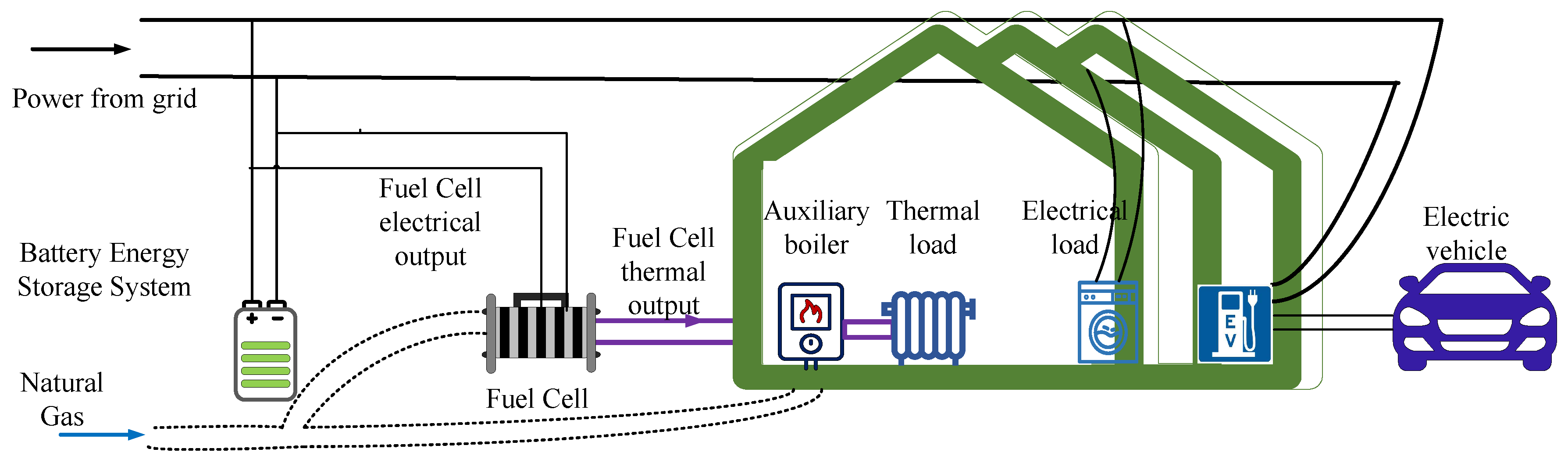
A typical SH having hybrid energy resources such as natural gas and electric power is presented in Figure 1. The energy flow in the SH is divided into two loops.
Thermal Loop:
It consists of thermal loads, an auxiliary boiler, and recovered heat from an FC. The energy source for the FC and auxiliary boiler is natural gas. The waste heat from the FC is recovered and provided to the thermal loads. If the heat provided by the FC is not sufficient to meet the total thermal power demand, the deficit power is provided by the auxiliary boiler.
Electrical Loop:
It consists of responsive and non-responsive electrical loads and electrical power resources (i.e., utility, FC, and BESS). The charging and discharging of the BESS depends upon its efficiency and the energy already stored in it according to the developed optimization model (as explained in Section 4). Modeling of the components of an SH is presented as follows.
2.1. FC Model
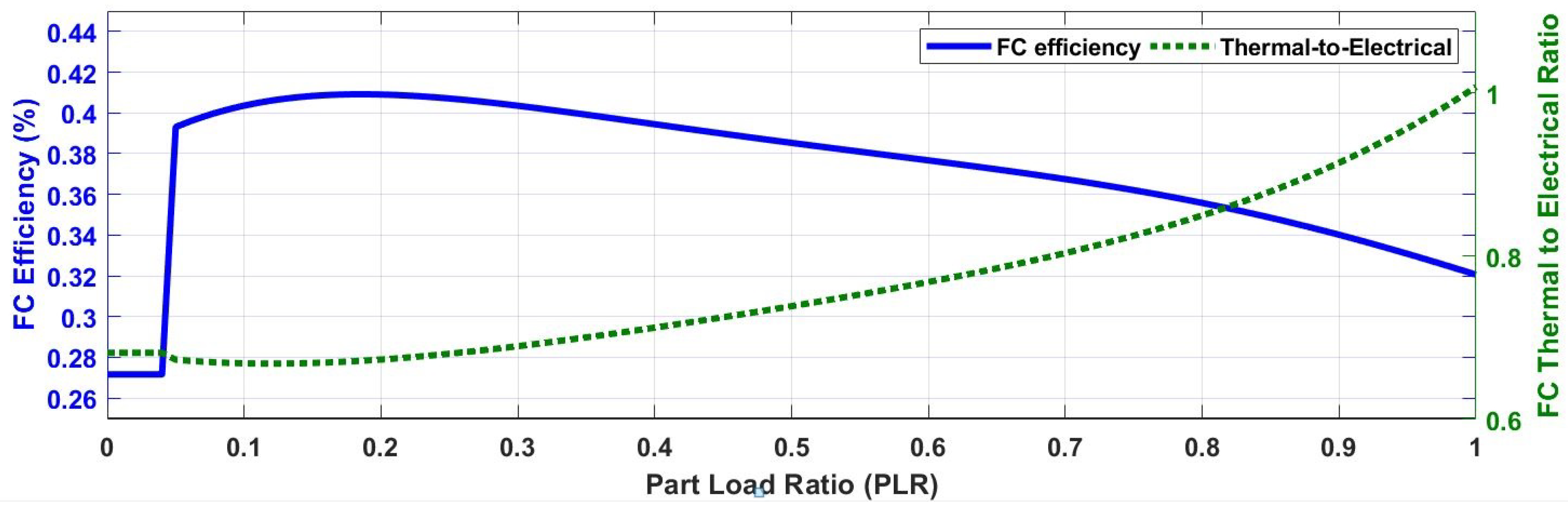
There are several types of FCs depending upon the fuel used for energy conversion. In this work, a proton exchange membrane fuel cell (PEM-FC) [30,31] is used. Serving as a micro-CHP system for the SH, input of the FC is natural gas and its outputs are electricity and heat. Efficiency of the FC is related to its part load ratio (PLR). PLR is the ratio of the electrical output at interval i to maximum power rating of the FC and is given in Equation (1):
where is the PLR at interval i when the FC output power is . Mathematical relations for the efficiency and thermal to electric ratio (rTE) are given as follows.
When :
When :
Having , the thermal power produced by the FC at interval i is calculated as:
Figure 2 represents typical performance characteristics of an FC [32]. At very low PLR (<10%), the parasitic losses are high and the overall efficiency is very low. Beyond this region, the FC operates at 30–40% electrical efficiency. The efficiency is slightly higher at lower PLR compared to the peak power operation. However, the performance and efficiency vary for different designs of FCs.
2.2. EV Model
To model the battery of an EV, several factors are required to be considered. These factors include the state of charge (SOC) at plug-out time, driving distance, driving style, route choice, traffic, etc. In this study, the data available in [33,34] is used. The effect of driving distance on SOC of battery is modeled as follows [24]:
where
| PEVi | EV charging power at interval i (kW) |
| SOCEV.i | EV SOC at interval i (%) |
| SOCEVpi | EV SOC at plugging-in time (%) |
| SOCEVpo | EV SOC at plugging-out time (%) |
| SOCEVmin | Minimum SOC of the EV (%) |
| d | Trip distance of the EV |
| ηEV | Overall electric drive efficiency |
| CEV | Capacity of the EV (kWh) |
If d and are given, the can be calculated using Equation (6). The is lower-bounded by the minimum SOC of the EV, which prevents the depletion damage to the EV battery.
The charging of EV is expressed as follows
2.3. BESS Model
The model of a BESS is provided in Equation (8). The charging and discharging efficiencies of the battery are considered in this work and the net BESS efficiency is 90%.
where is energy of the BESS at interval i, and denotes the power vector with the BESS charging and discharging powers, and are the charging and discharging efficiencies of the BESS, and T is the simulation step.
2.4. TOU Tariff
A TOU tariff refers to the different prices of electricity at different hours. Typically, the power demand is higher during certain time intervals of a day causing the overloading of a power grid. The utility companies set a higher price of electricity during these intervals to reduce stress on the power system. On the other hand, a lower price at some other intervals attracts the consumers and improves the utilization factor. In this work, the tariff considered for the SH is a peak-valley tariff which is a type of the TOU tariff. Three different prices of electricity are considered in this work during peak, plain and valley hours [35]. The price of electricity during these intervals is listed in Table 1 with their corresponding time intervals [36]. The price is normalized with respect to the maximum price defined in the peak period. These normalized values are used in Equation (12).
3. Optimization Model
This section presents the optimization model for the SH. The goal of the proposed optimization model is to minimize the 24 h operating costs of the SH subject to the following assumptions:
- The forecasted data for the thermal and electrical loads is available.
- The initial conditions of the SOC of the BESS and trip distance of the EV is available.
- All the devices are already installed. Therefore, the installation costs are not considered.
3.1. Objective Function
The objective function to be minimized is modeled as
where
where
| n | Number of hours |
| T | Length of a time interval (h) |
| α,β | Startup, Shutdown costs of the FC |
| CFC.i | Cost of the FC operation for interval i kWh) |
| CBL.i | Cost of the boiler operation for interval i kWh) |
| CU.i | Cost of the utility power for interval i kWh) |
| Cgas | Cost for purchasing the gas kWh) |
| CUb | Base cost for purchasing the power from utility |
| PFCe.i | Electrical power from the FC at interval i (kW) |
| PBL.i | Heating provided by the boiler at interval i (kW) |
| PU.i | Electrical power provided by the utility at interval i (kW) |
| Tp.v | Multiplier for the peak-valley price as provided in Table 1 |
| ηFC.i | Efficiency of the FC |
3.2. Constraints
Due to physical and operational limits of the devices and energy systems, the variables for power, energy and SOC should meet the following constraints during the optimization process.
3.2.1. Constraints of Power Balance
Electrical Power Balance
The input power from the utility is distributed among the electrical loads. The BESS either works as a source of electric power or an electric load. Therefore, following equations model the electrical power balance and this dual role of BESS.
When the BESS is charging:
When the BESS is discharging:
where
| Electrical demand at interval i (kW) | |
| Power being delivered to the EV at interval i (kW) | |
| BESS power at interval i (kW). It is negative in charging mode and positive in discharging mode | |
| Heating demand at interval i (kW) | |
| Heating produces by the FC at interval i (kW) | |
| Charging efficiency of the BESS | |
| Discharging efficiency of the BESS |
Thermal Power Balance
The total demand of thermal power is met by the FC and the auxiliary boiler in the SH. The constraint of thermal power balance is formulated as:
where
| PDh.i | Heating demand at interval i (kW) |
| PFCh.i | Heating produced by the FC at interval i (kW) |
| PBL.i | Heating produced by the auxiliary boiler at interval i (kW) |
3.2.2. Constraints of Devices
The constraints applicable to the devices available in the SH are explained below.
Constraints of FC
The rate of change of the FC output is limited to the upper and the lower boundaries of ramp rate. Therefore, following inequalities must be satisfied:
where
| ΔPFCup | FC ramp rate limit for increasing power |
| ΔPFCdn | FC ramp rate limit for decreasing power |
| PFCmin | FC minimum power limit |
| PFCmax | FC maximum power limit |
Constraints of EV
Charging and discharging of the EV battery is subject to certain limitations regarding its maximum charging power and the SOC as given below:
where is the maximum charging power of the EV in (kW) and is the maximum SOC.
Constraints of BESS
Following constraints the BESS must be satisfied:
If the battery is in charging/discharging mode, it is subjected to the maximum charging and discharging rates as explained below:
During Charging Mode
During Discharging Mode
where
| WB.i | BESS energy at interval i (kWh) |
| WBmin | BESS minimum energy limit (kWh) |
| WBmax | BESS maximum energy limit (kWh) |
| PBchmax | BESS minimum charging rate limit (kW) |
| PBdchmax | BESS maximum discharging rate limit (kW) |
| T | Length of time interval |
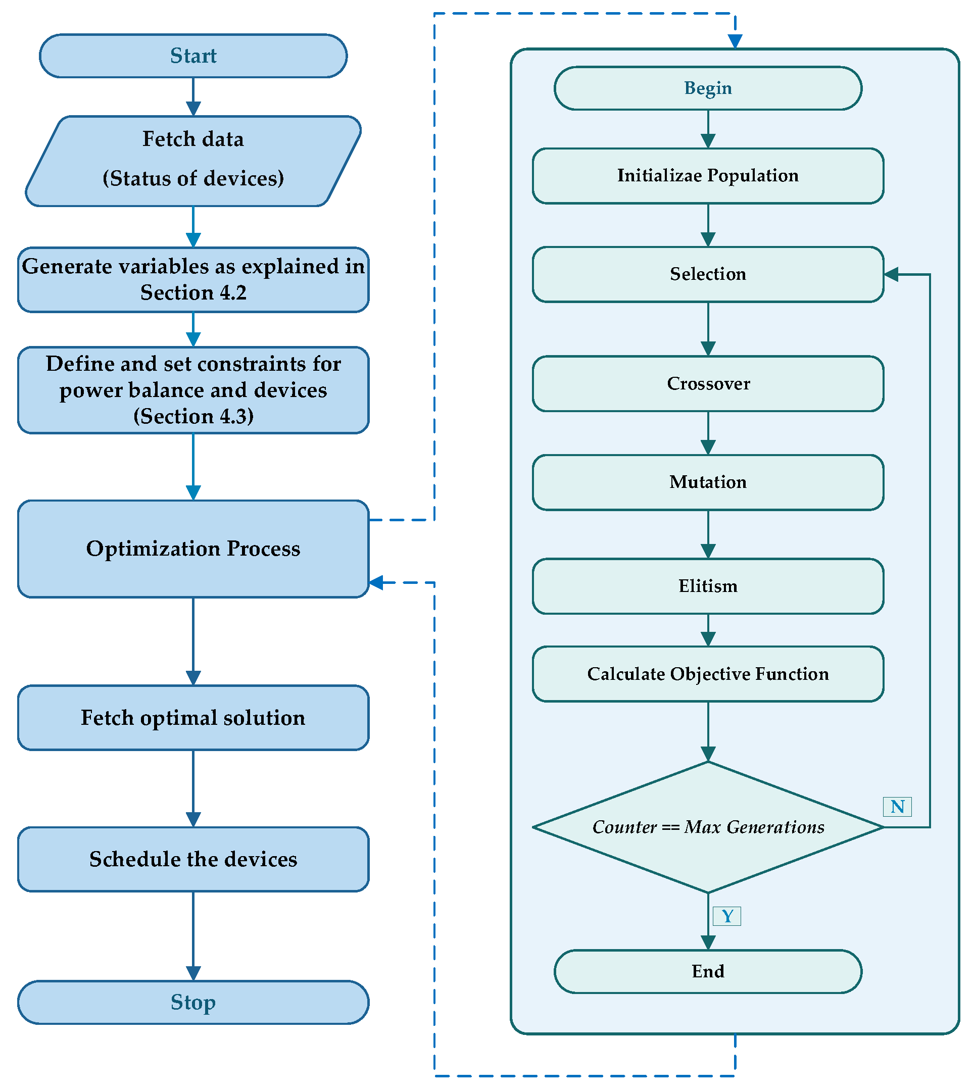
4. Real Coded Genetic Algorithm
Modern heuristic techniques are fast and emerging tools to optimize non-linear systems. Generally, they outperform the traditional derivative based techniques which have limitations of getting trapped in a local minimum, computational complexity, or are not applicable to certain objective functions. The Genetic Algorithm (GA) is one of the most used evolutionary algorithms in power system applications. Its mechanism is based on evolution in nature and the algorithm essentially consists of genetic operations of selection, cross-over and mutation applied to a population of chromosomes. RCGA which is an improved version of the GA is implemented in this study for the optimization purpose. For real valued numerical optimization problems, the floating point or integer representation of population variables in RCGA outperforms the binary representation of the variables in the GA. In comparison to the GA, the RCGA provides higher consistency, more precision and faster convergence [37].
RCGA is an efficient method which does not require a derivative of the objective function to find the optimal solution. Therefore, in contrast to the linear programming or derivative-based techniques, RCGA can effectively handle all types of objective functions and constraints whether they are smooth, non-smooth; linear, non-linear; continuous, discontinuous; convex, non-convex; stochastic or does not possess derivatives. A detailed discussion of the RCGA is available in [38,39,40]. A brief description of the steps involved in the implementation of the RCGA for optimal scheduling of the SH’s energy resources is presented below.
4.1. Initialization
Similar to other evolutionary algorithms, the RCGA starts with generation of an initial population called “chromosomes”. In an N-dimensional optimization problem, the position of i-th gene is determined as follows:
where each gene denotes power (kW) of a device and is total number of genes in a chromosome.
4.2. Dimensionality
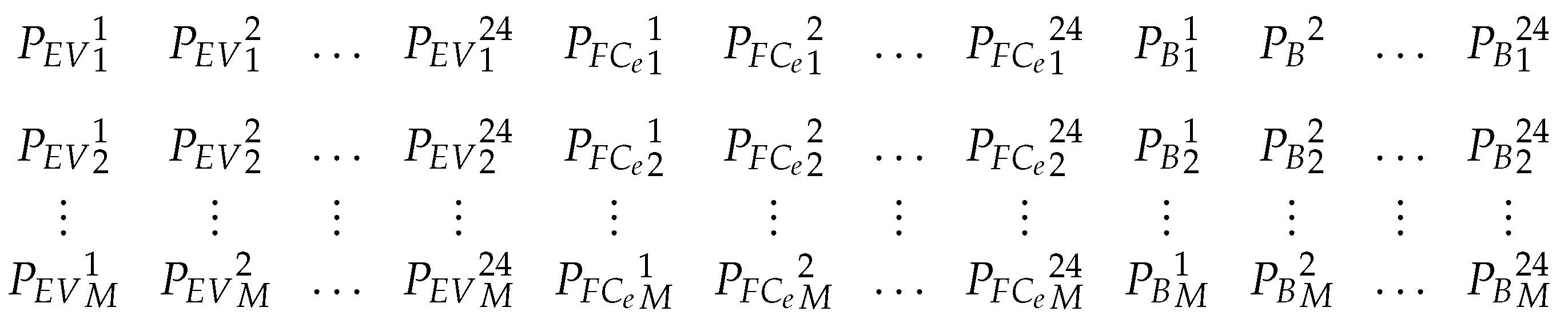
The number of independent variables in a system determines the dimensions of an optimization problem. For the SH presented in this work, there are three independent variables namely , and . The information of these independent variables and power demands of the thermal and electrical loads are used to determine all the remaining unknown variables. For example, knowing , can be solved using Equations (2)–(5). Similarly, and can be computed using Equations (13)–(15). The objective of this study is to calculate an optimal scheduling of SH devices for one day (24 h) with a time interval of h. Therefore, three variables in each hour result in the dimension of optimization problem .
If M is the number of chromosomes in one generation then gives the dimensionality in terms of one generation of the RCGA as shown in Figure 3.
4.3. Implementation of the Constraints
In each time interval, all the system constraints for and are checked as follows:
- Constraints of FC
- Constraints of the BESS
- For each interval i, if exceeds the battery capacity limit in charging mode i.e., , then and h to satisfy the upper limit of (21).
- For each interval i, if depletes more than battery minimum limit in discharging mode, i.e., then and to satisfy the lower limit of (21).
- If the battery is in charging mode i.e., , then the difference between values of battery energy in two consecutive intervals should not exceed according to (22). Otherwise h.
- If the battery is in discharging mode i.e., , then the difference between the values of battery energy in two consecutive intervals should be less than according to (23). Otherwise h.
- Constraints of the EV
The flowchart of the RCGA-based optimal scheduling process is shown in Figure 4.
5. Simulation Results
This section presents the results of the numerical simulations to highlight the significant features of the proposed optimization model. As the SH has hybrid energy resources and is equipped with various devices, therefore, multiple simulation scenarios are generated to compare their impacts under different utility tariffs as shown in Table 1. In all the simulation scenarios, the electric power can be purchased from the utility and the auxiliary boiler is available for the thermal energy. Table 2 presents these cases.
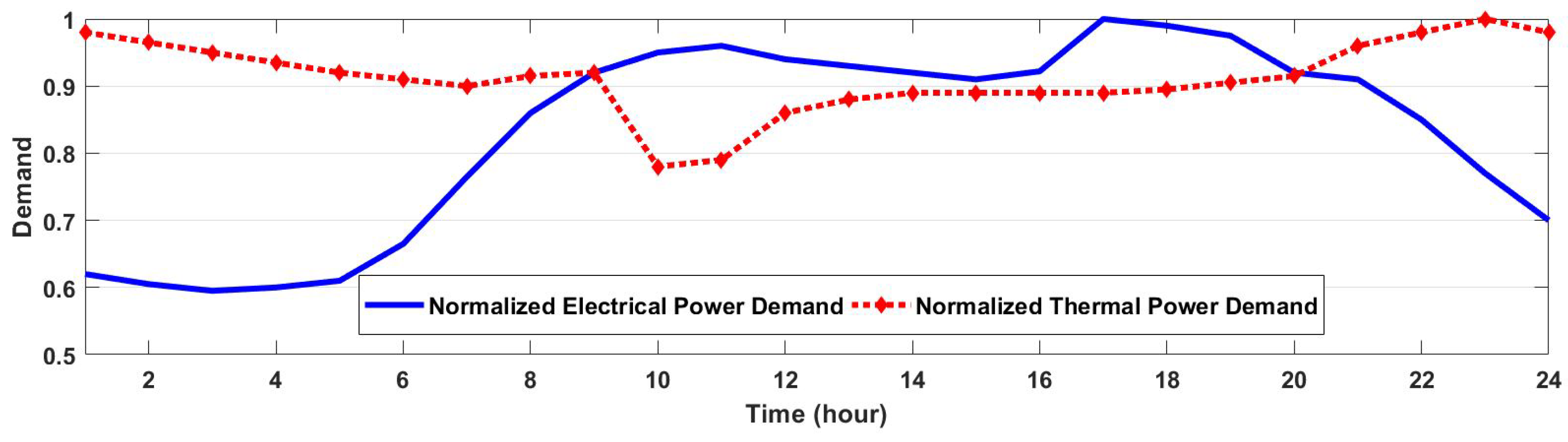
The normalized curves for the 24 h thermal and electric power demands of the SH are shown in Figure 5 [41]. The thermal demand curve is relatively stable with mean to peak ratio of 91.5% whereas the electrical power demand curve is fluctuating and its mean to peak ratio is 83%. To meet the load demands, the proposed optimization model finds the optimal resources for the 24 h operation of the SH. The electrical resources need more attention due to significantly changing profile of the electrical power demand. The heat and electricity demands are 2.5 kW each for the SH. The cost is calculated for the 24 h. The micro-CHP system follows the electrical demand to generate the electricity while delivering the heat as a by-product. The EV used in this study is Mitsubishi’s compact i-MiEV [42]. It can travel 62 miles on a full charge in typical driving conditions. The distance traveled by the EV, time-in and time-out are selected according to the U.S. National House-hold Travel Survey (NHTS) [33,34]. A smart charging mechanism for the EV and BESS is considered which charges them according to the optimized values generated by the proposed optimization model based on the RCGA. All the parameters related to the SH, EV, FC, BESS, and optimization model are given in Table 3.
5.1. Case 1: Base Case
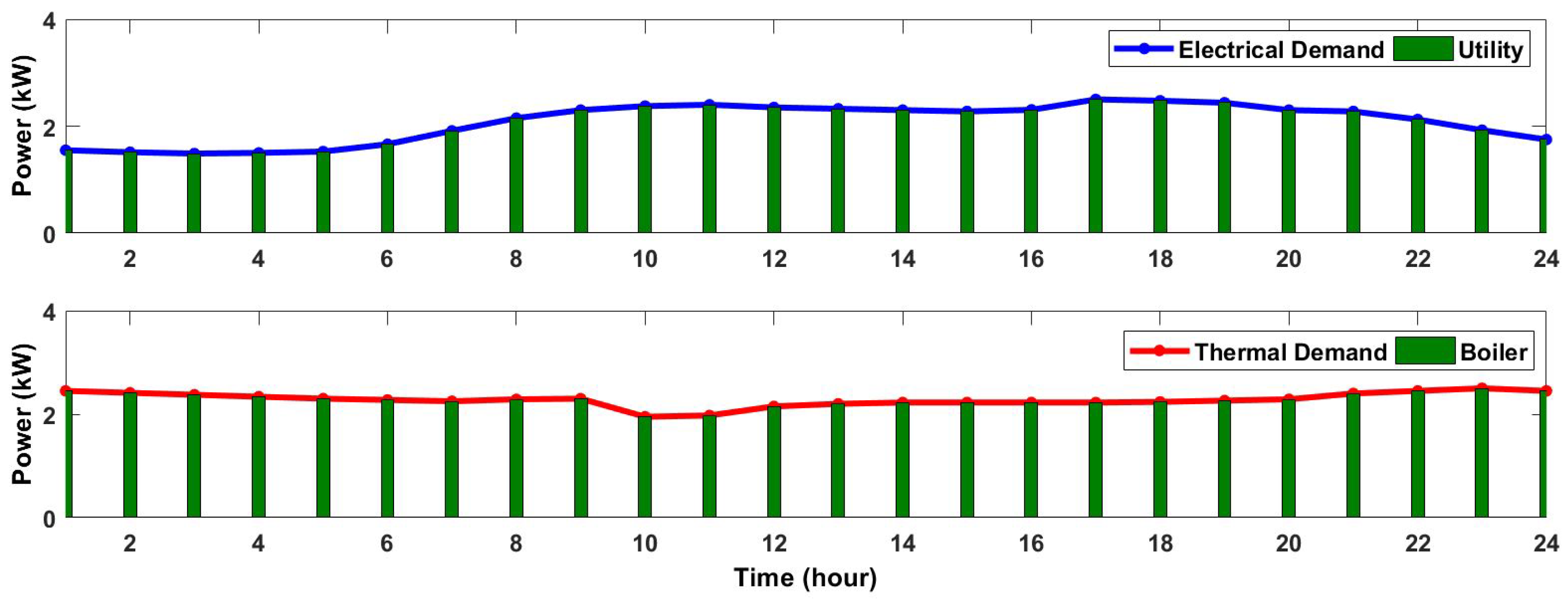
Case 1 serves as a base case which represents a typical conventional home without a micro-CHP and an EV. As shown in Table 3, this case does not consider availability of the BESS at the home, and the variable tariff is not applied. The proposed optimization model is not applicable to this case. The non-schedulable electric demand of the home is met by the utility, and the thermal demand is met by the boiler as shown in Figure 6. In this case, the total cost of the energy is 9.20 ($/day).
5.2. Case 2: Installation of FC
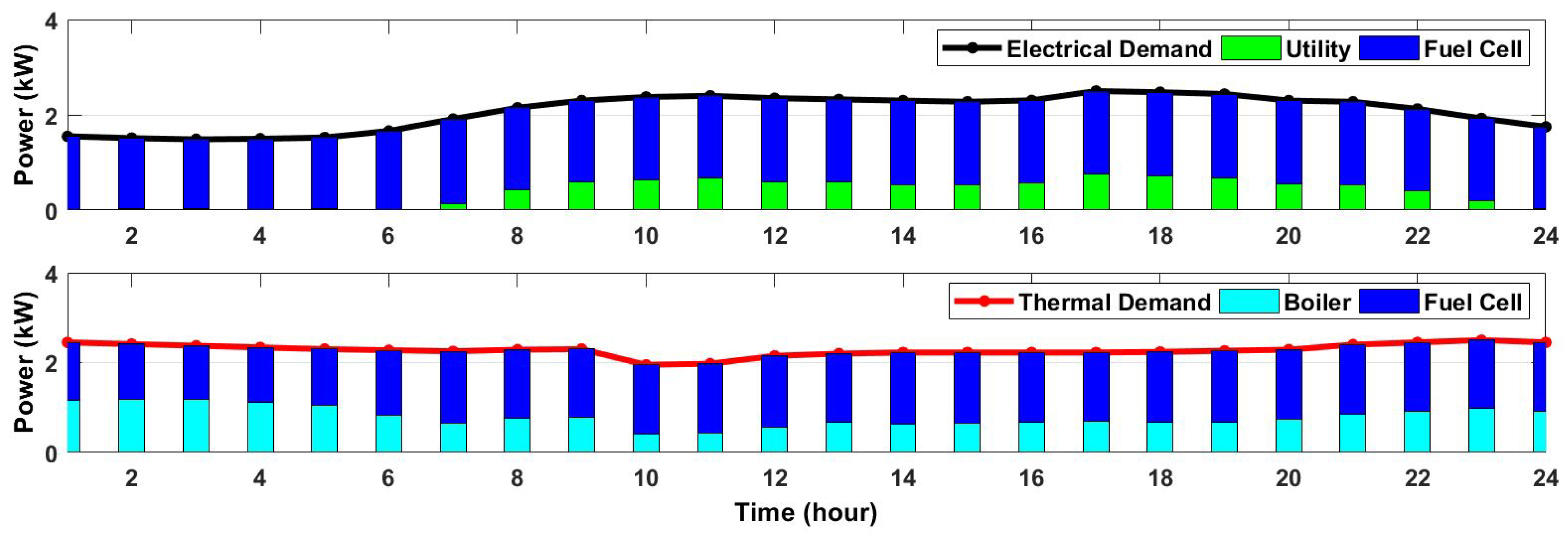
In this case, an FC is added to the SH which serves as a micro-CHP system, and a significant portion of electric and thermal loads shifts to it due to its economic operation. Due to the power rating of the FC, it cannot meet the whole electric power demand of the SH and a part of electric energy is purchased from the utility. Similarly, the auxiliary boiler provides the additional heating if the thermal power demand is more than the FC’s thermal power output. Figure 7 shows the results for the optimal dispatch of the FC, utility and auxiliary boiler. It is observed that FC follows the electrical load curve in the night hours when demand is low. During the day, the FC works at near its maximum power generation limit. The remaining power is provided by the utility. No variable tariff is considered at this point, and the FC output is almost constant for 24 h. Another important point is that the FC is not working exactly at its maximum power generation capacity. According to (3), if the FC generates maximum power, its efficiency decreases and the total operational cost becomes higher than the cost of purchasing from the utility. The net cost is 7.97 ($/day) in this case which is 13.37% less as compared to the cost incurred in Case 1 when there was no micro-CHP in the SH.
5.3. Case 3: Addition of EV
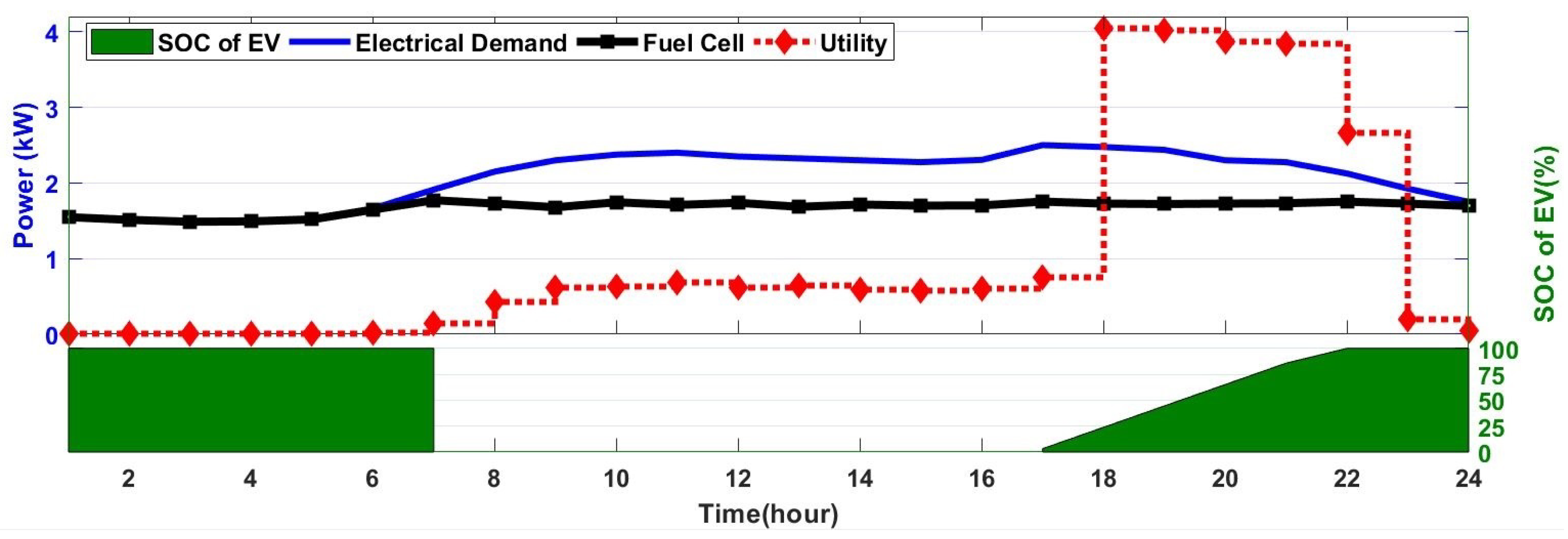
In this case, an EV is added to the SH and its impact is analyzed. This case considers the EV as a constant and unscheduled load. Thus, depending upon the initial SOC of EV, it presents itself as a constant load from the time it is plugged-in until it gets fully charged. Figure 8 shows the SOC of EV battery and electric powers from the utility and FC in this case. The operating cost of the system is 9.98 ($/day) which is higher than Case 2 due to the loading effect of the EV.
5.4. Case 4: Considering Variable Tariff
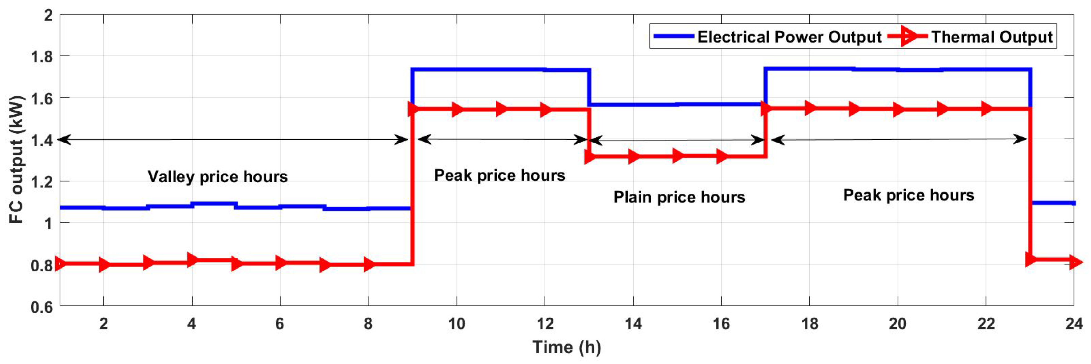
In the previous cases, the utility tariff was considered as flat rates for 24 h. This case and the following cases, however, consider a variable tariff which is widely applicable in the present power markets. A peak-valley tariff is considered in this case according to Table 1. As shown in Figure 9, EV loading on the system is the same as in Case 3 but the FC adjusts its output to take benefit of the valley prices. To achieve an economic operation, the proposed optimization algorithm makes the FC increase its output during peak price hours and reduce its output during valley price hours. This is in contrast to Case 2 when the FC was operating on almost constant output for 24 h. Due to the exploitation of variable tariff by the optimization model, the total system cost has decreased to 9.88 ($/day).
5.5. Case 5: Scheduling the EV Charging
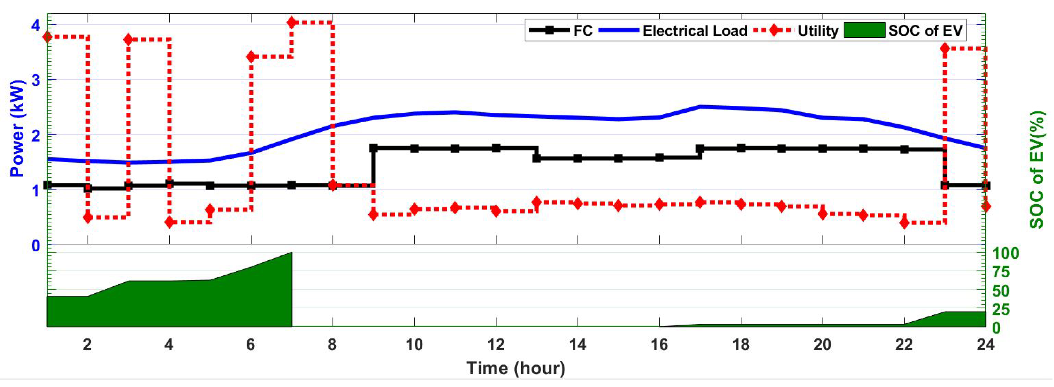
The modern concept of scheduling of responsive electric loads results in great economic and technical benefits [43,44]. The electric loads of high power rating and low criticality such as EV, washing machines are the prime candidates for such scheduling. In this case, the EV is modeled as a responsive load and its charging is scheduled. The optimization algorithm selects those hours for the EV charging when the total cost is optimized and the EV is fully charged. Figure 10 shows the EV charging hours, SOC of the EV battery, and electric powers from the utility and the FC in this case.
Although EV is connected to the system as soon as it reaches the house at 5:00 P.M., the optimization algorithm forced it to charge during those hours when the customer can get more benefit. The charging of EV starts from 11:00 P.M. (during valley prices) and the SOC reaches up to 100% before EV leaves home at 7:00 A.M. The cost reduces to 9.44 ($/day) which is around 5% decrease as compared to Case 4.
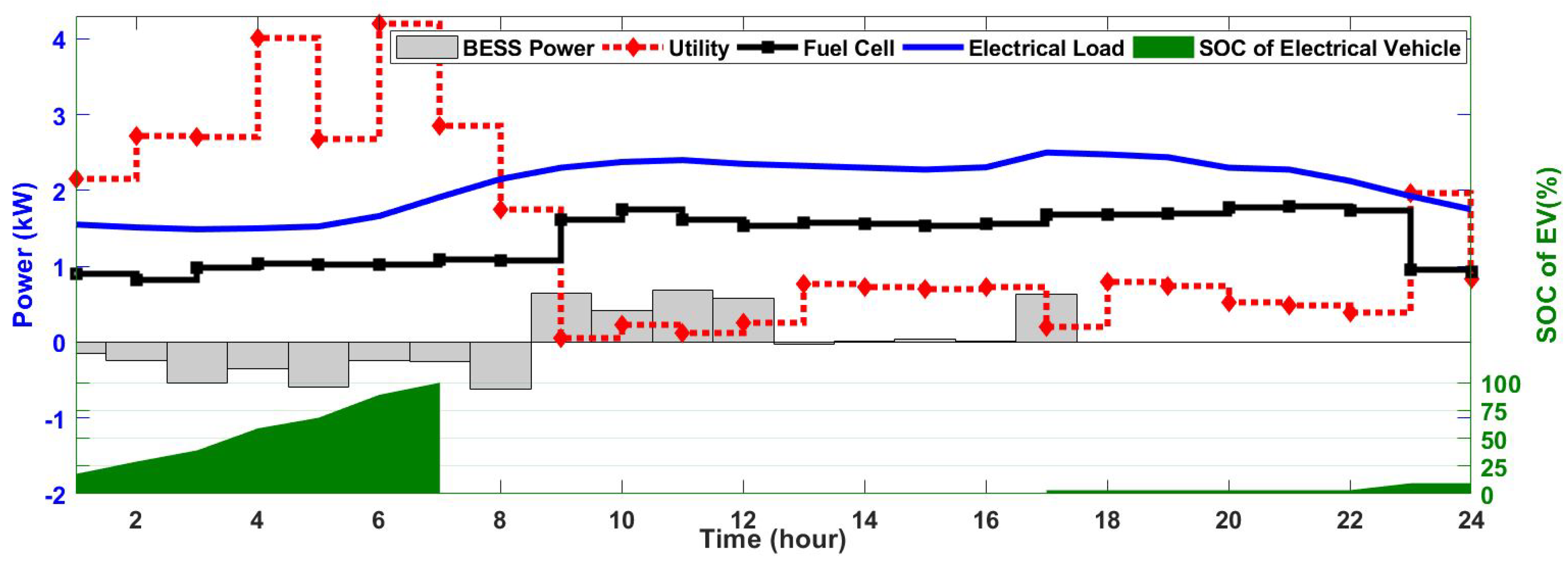
5.6. Case 6: Adding the BESS
This case considers the addition of a BESS to the SH and analyzes its impacts. It is notable that using the BESS with the utility can result in an economic operation only if the product of charging and discharging efficiencies is greater than the valley-to-peak price ratio. In this case, BESS is charged during the valley price hours and discharged during the peak price hours. Therefore, it is pertinent to introduce BESS efficiency in this section which is . In this work, BESS efficiency () is 0.9, and charging and discharging of BESS is shown in Figure 11. The product of the two efficiencies is more than the valley-to-peak price ratio of the utility tariff therefore energy routing through BESS can result in economic operation. However, to exploit the maximum benefit from BESS, the proposed optimization algorithm selects its charging and discharging hours as explained below.
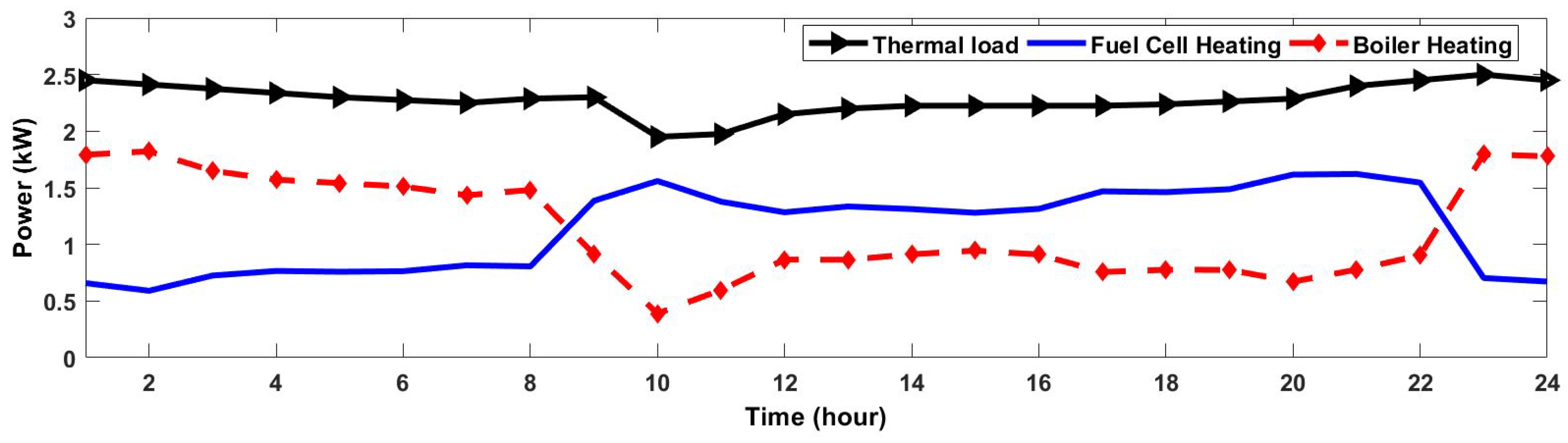
The utility tariff is at its lowest price during 01:00–08:00, therefore BESS is charged. The FC does not operate at its maximum because it generates electricity such that its cost per unit is lower than or equal to utility. Energy share provided by the utility is maximum during this interval. The charging of BESS at this tariff results in 0.8667 p.u/kW of the dischargeable energy. For thermal demand, most of the heating is provided by the boiler, and FC adds to some extent as shown in Figure 12.
From 09:00–12:00, utility tariff is at its maximum price. The proposed optimization algorithm results in low purchase from the utility, discharging of the BESS to deliver power to electric loads, and increased output of the FC. This results in an increased thermal output from FC, and heating from the boiler is lowered. The FC does not produce power exactly equal to its maximum generation capacity as discussed in Case 2 Section 5.2.
The utility tariff is at plain price during 13:00–16:00. This interval needs special attention as the proposed optimization model yields interesting results during this time interval. The BESS has options of either charging or discharging. Charging 1 kW at this interval with the 0.9 BESS efficiency results in 0.9 kW of discharge-able energy at the rate of 1 p.u./kW (0.9 p.u./0.9 kW). This rate is similar to the utility price of 1 p.u. at the interval 17:00–22:00. Charging in this interval does not result in any cost benefit for the system, and RCGA manages not to charge the BESS. On the other hand, discharging during this interval can result in cost reduction. However, the optimization algorithm weighs comparatively either to discharge during this interval or during 17:00–22:00. Discharging during a later interval saves more, therefore the BESS does not discharge during 13:00–16:00. In this way, the overall economy is optimized. Moreover, the electrical as well as thermal output of the FC is decreased to get benefit from the reduced tariff during this interval as shown in Figure 11.
Due to the peak price tariff during 17:00–22:00, a minimum energy is purchased from the utility. The BESS discharges and the FC increases its output to meet the energy demand. In the hours 23:00–24:00, the SH’s electrical and thermal powers follow the trends already discussed in the interval 1 to 8.
The net cost of operation is day) in this case according to (9) which is less than the cost obtained in Case 5. Similar to Case 5, the scheduled charging of EV is considered in this case as well. It is notable that EV charging pattern in Figure 11 is different to that given in Figure 10. This is due to the fact that RCGA generates new random population for each simulation. No effort is made to reserve the randomness of the simulation process. Nevertheless, the EV is getting charged in valley hours in both cases and reaches to the before leaving the SH.
6. Conclusions
The modern SHs are foreseen to have an increased use of micro-CHP systems and availability of hybrid energy resources. This work presented a model of an SH and provided an algorithm for optimal scheduling of hybrid energy resources to minimize the cost of 24 h energy consumption. The findings of six different simulation scenarios reveal that the micro-CHP systems and the responsive electrical loads can play a vital role in reduction of the total energy cost. The conditions for the feasible use of BESS are also explained. The proposed optimization model based on successfully convergent RCGA makes use of the variable tariff and manipulates the devices for an optimal energy cost under the provided constraints. The presented work provides a comprehensive structure for hybrid energy management of a SH and can serve as a basis for further research. Further work can be carried out using a bidirectional utility grid, including thermal energy storage systems and integration of renewable energy resources.
Author Contributions
M.K.R. conceived the idea and did preliminary work. C.-H.K. provided guidelines necessary to complete the work. Z.M.H., M.I., and K.K.M. helped in code development. M.S.U.Z. and S.U.K. helped during paper writing and reviewing process.
Funding
This research was funded by National Research Foundation of Korea (NRF) grant funded by the Korea government (MSIP), grant number 2018R1A2A1A05078680” and “The APC was funded by the Authors”.
Conflicts of Interest
The authors declare no conflict of interest.
References
- Combined Heat and Power(CHP). Available online: http://aceee.org/topics/combined-heat-and-power-chp (accessed on 25 December 2016).
- Liu, L.; Liu, Y.; Wang, L.; Zomaya, A.; Hu, S. Economical and balanced energy usage in the smart home infrastructure: A tutorial and new results. IEEE Trans. Emerg. Top. Comput. 2015, 3, 556–570. [Google Scholar] [CrossRef]
- Nyboer, J.; Groves, S.; Baylin-Stern, A. A Review of Existing Cogeneration Facilities in Canada; Technical Report; Canadian Industrial Energy End-Use Data and Analysis Centre, Simon Fraser University: Burnaby, BC, Canada, 2013. [Google Scholar]
- Aki, H. The Penetration of Micro CHP in Residential Dwellings in Japan. In Proceedings of the 2007 IEEE Power Engineering Society General Meeting, Tampa, FL, USA, 24–28 June 2007; pp. 1–4. [Google Scholar]
- Houwing, M.; Negenborn, R.R.; Schutter, B.D. Demand Response With Micro-CHP Systems. Proc. IEEE 2011, 99, 200–213. [Google Scholar] [CrossRef] [Green Version]
- Karami, H.; Sanjari, M.J.; Hosseinian, S.H.; Gharehpetian, G.B. An Optimal Dispatch Algorithm for Managing Residential Distributed Energy Resources. IEEE Trans. Smart Grid 2014, 5, 2360–2367. [Google Scholar] [CrossRef]
- Murugan, S.; Horák, B. A review of micro combined heat and power systems for residential applications. Renew. Sustain. Energy Rev. 2016, 64, 144–162. [Google Scholar] [CrossRef]
- Benam, M.R.; Madani, S.S.; Alavi, S.M.; Ehsan, M. Optimal Configuration of the CHP System Using Stochastic Programming. IEEE Trans. Power Deliv. 2015, 30, 1048–1056. [Google Scholar] [CrossRef]
- Xie, D.; Lu, Y.; Sun, J.; Gu, C.; Li, G. Optimal Operation of a Combined Heat and Power System Considering Real-time Energy Prices. IEEE Access 2016, 4, 3005–3015. [Google Scholar] [CrossRef]
- Adam, A.; Fraga, E.S.; Brett, D.J. Options for residential building services design using fuel cell based micro-CHP and the potential for heat integration. Appl. Energy 2015, 138, 685–694. [Google Scholar] [CrossRef]
- Feng, Z.-B.; Jin, H.-G. Part-load performance of CCHP with gas turbine and storage system. Proc. CSEE 2006, 26, 25–30. [Google Scholar]
- El-Sharkh, M.Y.; Rahman, A.; Alam, M.S.; El-Keib, A.A. Thermal energy management of a CHP hybrid of wind and a grid-parallel PEM fuel cell power plant. In Proceedings of the 2009 IEEE/PES Power Systems Conference and Exposition, Washington, DC, USA, 15–18 March 2009; pp. 1–6. [Google Scholar]
- Nehrir, M.H.; Wang, C. Hybrid Fuel Cell Based Energy System Case Studies. In Modeling and Control of Fuel Cells: Distributed Generation Applications; Wiley-IEEE Press: Hoboken, NJ, USA, 2009; pp. 219–264. [Google Scholar]
- Romano, R.; Siano, P.; Acone, M.; Loia, V. Combined Operation of Electrical Loads, Air Conditioning and Photovoltaic-Battery Systems in Smart Houses. Appl. Sci. 2017, 7, 525. [Google Scholar] [CrossRef]
- Angrisani, G.; Canelli, M.; Roselli, C.; Sasso, M. Integration between electric vehicle charging and micro-cogeneration system. Energy Convers. Manag. 2015, 98, 115–126. [Google Scholar] [CrossRef]
- Wakui, T.; Wada, N.; Yokoyama, R. Energy-saving effect of a residential polymer electrolyte fuel cell cogeneration system combined with a plug-in hybrid electric vehicle. Energy Convers. Manag. 2014, 77, 40–51. [Google Scholar] [CrossRef]
- Wakui, T.; Wada, N.; Yokoyama, R. Feasibility study on combined use of residential SOFC cogeneration system and plug-in hybrid electric vehicle from energy-saving viewpoint. Energy Convers. Manag. 2012, 60, 170–179. [Google Scholar] [CrossRef]
- Ribberink, H.; Entchev, E. Exploring the potential synergy between micro-cogeneration and electric vehicle charging. Appl. Therm. Eng. 2014, 71, 677–685. [Google Scholar] [CrossRef]
- Yao, L.; Damiran, Z.; Lim, W.H. Optimal Charging and Discharging Scheduling for Electric Vehicles in a Parking Station with Photovoltaic System and Energy Storage System. Energies 2017, 10, 550. [Google Scholar] [CrossRef]
- Mohsenian-Rad, H.; Ghamkhari, M. Optimal Charging of Electric Vehicles With Uncertain Departure Times: A Closed-Form Solution. IEEE Trans. Smart Grid 2015, 6, 940–942. [Google Scholar] [CrossRef]
- Cao, Y.; Tang, S.; Li, C.; Zhang, P.; Tan, Y.; Zhang, Z.; Li, J. An Optimized EV Charging Model Considering TOU Price and SOC Curve. IEEE Trans. Smart Grid 2012, 3, 388–393. [Google Scholar] [CrossRef] [Green Version]
- Jin, C.; Sheng, X.; Ghosh, P. Energy efficient algorithms for Electric Vehicle charging with intermittent renewable energy sources. In Proceedings of the 2013 IEEE Power Energy Society General Meeting, Vancouver, BC, Canada, 21–25 July 2013; pp. 1–5. [Google Scholar] [CrossRef]
- Bhatti, A.R.; Salam, Z. A rule-based energy management scheme for uninterrupted electric vehicles charging at constant price using photovoltaic-grid system. Renew. Energy 2018, 125, 384–400. [Google Scholar] [CrossRef]
- Wu, X.; Hu, X.; Yin, X.; Moura, S. Stochastic Optimal Energy Management of Smart Home with PEV Energy Storage. IEEE Trans. Smart Grid 2016, 9, 2065–2075. [Google Scholar] [CrossRef]
- García-Villalobos, J.; Zamora, I.; San Martín, J.I.; Asensio, F.J.; Aperribay, V. Plug-in electric vehicles in electric distribution networks: A review of smart charging approaches. Renew. Sustain. Energy Rev. 2014, 38, 717–731. [Google Scholar] [CrossRef]
- Khan, S.U.; Mehmood, K.K.; Haider, Z.M.; Bukhari, S.B.A.; Lee, S.J.; Rafique, M.K.; Kim, C.H. Energy Management Scheme for an EV Smart Charger V2G/G2V Application with an EV Power Allocation Technique and Voltage Regulation. Appl. Sci. 2018, 8, 648. [Google Scholar] [CrossRef]
- Dubey, A.; Santoso, S. Electric Vehicle Charging on Residential Distribution Systems: Impacts and Mitigations. IEEE Access 2015, 3, 1871–1893. [Google Scholar] [CrossRef]
- Qayyum, F.; Naeem, M.; Khwaja, A.S.; Anpalagan, A.; Guan, L.; Venkatesh, B. Appliance scheduling optimization in smart home networks. IEEE Access 2015, 3, 2176–2190. [Google Scholar] [CrossRef]
- Javaid, N.; Ahmed, A.; Iqbal, S.; Ashraf, M. Day Ahead Real Time Pricing and Critical Peak Pricing Based Power Scheduling for Smart Homes with Different Duty Cycles. Energies 2018, 11, 1464. [Google Scholar] [CrossRef]
- Nedstack. Product Specifications of XXL Stacks; Nedstack: Arnhem, The Netherlands, 2014. [Google Scholar]
- El-Sharkh, M.Y.; Tanrioven, M.; Rahman, A.; Alam, M.S. A study of cost-optimized operation of a grid-parallel PEM fuel cell power plant. IEEE Trans. Power Syst. 2006, 21, 1104–1114. [Google Scholar] [CrossRef]
- Gunes, M.B. Investigation of a Fuel Cell Based Total Energy System for Residential Applications. Master’s Thesis, University in Blacksburg, Blacksburg, VA, USA, 2001. [Google Scholar]
- National Household Travel Survey. Electric Vehicle Feasibility: Can EVs Take US Households to Where They Need to Go? Technical Report; National Household Travel Survey: Washington, DC, USA, 2016.
- National Household Travel Survey. Summary of Travel Trends; Technical Report; National Household Travel Survey, Department of Transportation: Washington, DC, USA, 2009.
- Hu, Z.; Han, X.; Wen, Q. Integrated Resource Strategic Planning and Power Demand-Side Management; Power Systems; Springer: Berlin, Germany, 2013. [Google Scholar]
- Gianfreda, A.; Grossi, L. Zonal price analysis of the Italian wholesale electricity market. In Proceedings of the 2009 6th International Conference on the European Energy Market, Leuven, Belgium, 27–29 May 2009; pp. 1–6. [Google Scholar] [CrossRef]
- Michalewicz, Z. Genetic Algorithms + Data Structures = Evolution Programs, 3rd ed.; Springer: London, UK, 1996. [Google Scholar]
- Damousis, I.G.; Bakirtzis, A.G.; Dokopoulos, P.S. Network-constrained economic dispatch using real-coded genetic algorithm. IEEE Trans. Power Syst. 2003, 18, 198–205. [Google Scholar] [CrossRef] [Green Version]
- Kuri-Morales, A.F.; Gutiérrez-García, J. Penalty Function Methods for Constrained Optimization with Genetic Algorithms: A Statistical Analysis. In MICAI 2002: Advances in Artificial Intelligence, Proceedings of the Second Mexican International Conference on Artificial Intelligence Mérida, Yucatán, Mexico, 22–26 April 2002; Coello Coello, C.A., de Albornoz, A., Sucar, L.E., Battistutti, O.C., Eds.; Springer: Berlin/Heidelberg, Germany, 2002; pp. 108–117. [Google Scholar] [CrossRef]
- Amjady, N.; Nasiri-Rad, H. Economic dispatch using an efficient real-coded genetic algorithm. IET Gener. Transm. Distrib. 2009, 3, 266–278. [Google Scholar] [CrossRef]
- Linkevics, O.; Sauhats, A. Formulation of the objective function for economic dispatch optimisation of steam cycle CHP plants. In Proceedings of the 2005 IEEE Russia Power Tech, St. Petersburg, Russia, 27–30 June 2005; pp. 1–6. [Google Scholar] [CrossRef]
- Mitsubihsi i-MiEV Specifications. Available online: https://www.mitsubishi-motors.com/en/showroom/i-miev/specifications/ (accessed on 20 December 2016).
- Saeed Uz Zaman, M.; Bukhari, S.B.A.; Hazazi, K.M.; Haider, Z.M.; Haider, R.; Kim, C.H. Frequency Response Analysis of a Single-Area Power System with a Modified LFC Model Considering Demand Response and Virtual Inertia. Energies 2018, 11, 787. [Google Scholar] [CrossRef]
- Haider, Z.M.; Mehmood, K.K.; Rafique, M.K.; Khan, S.U.; Soon-Jeong, L.; Chul-Hwan, K. Water-filling algorithm based approach for management of responsive residential loads. J. Mod. Power Syst. Clean Energy 2018, 6, 118–131. [Google Scholar] [CrossRef]
Figure 1.
Overview of a smart house.

Figure 2.
Fuel cell efficiency and thermal to electrical ratio as function of Part Load Ratio.

Figure 3.
Chromosomes in one generation of the real coded genetic algorithm.

Figure 4.
Flowchart of the proposed work.

Figure 5.
Daily thermal and electric power demands.

Figure 6.
Case 1: Basic operation mode of house.

Figure 7.
Case 2: Electrical and thermal demands after adding the fuel cell.

Figure 8.
Case 3: Charging of electric vehicle (EV) without scheduling.

Figure 9.
Case 4: Impact of peak-valley tariff on fuel cell output.

Figure 10.
Case 5: Results of the system with scheduling of EV.

Figure 11.
Case 6: Results of the simulation after adding battery energy storage system.

Figure 12.
Case 6: Thermal heating.

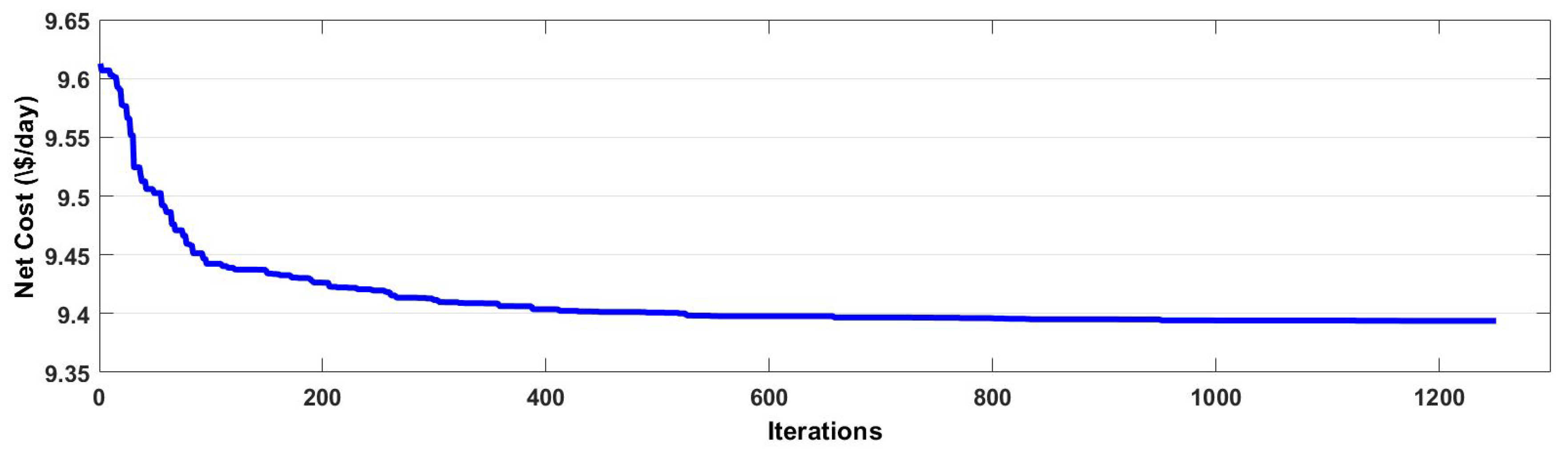
Figure 13.
Convergence of RCGA.

Table 1.
Peak-Valley Electricity Tariff.
| Tarrif Type | Time Range | Normalized Price |
|---|---|---|
| Peak | [09:00–12:00] | 1 |
| [17:00–22:00] | ||
| Plain | [13:00–16:00] | 0.9 |
| Valley | [01:00–08:00] | 0.78 |
| [23:00–24:00] |
Table 2.
Description of the test cases.
| Case No | FC | EV | Variable Tariff | Scheduling of EV | BESS |
|---|---|---|---|---|---|
| 1 | x | x | x | x | x |
| 2 | o | x | x | x | x |
| 3 | o | o | x | x | x |
| 4 | o | o | o | x | x |
| 5 | o | o | o | o | x |
| 6 | o | o | o | o | o |
Table 3.
System Parameters.
| Parameter Description | Value | Unit | |
|---|---|---|---|
| Electric Vehicle | |||
| Trip distance of EV | d | 60 | mi |
| Overall electric drive efficiecy | 6.2 | - | |
| Capacity of EV | 16 | kWh | |
| EV maximum charging power | 3.3 | kW | |
| Minimum SOC of EV | 3.3 | % | |
| Maximum SOC of EV | 100 | % | |
| EV SOC at plugging-out time | 100 | % | |
| Plug-in time | 17:00 | hour | |
| Plug-out time | 7:00 | hour | |
| Fuel Cell | |||
| FC maximum power limit | 2 | kW | |
| FC minimum power limit | 0.05 | kW | |
| FC ramp rate limit for increasing power | 1.25 | kW | |
| FC ramp rate limit for decreasing power | 1.5 | kW | |
| FC startup cost | 0.15 | $ | |
| FC shutdown cost | 0 | $ | |
| Battery Energy Storage System | |||
| Maximum energy limit | 3 | kWh | |
| Minimum energy limit | 0 | kWh | |
| Minimum charging rate limit | c/4 | kW | |
| Maximum discharging rate limit | c/2 | kW | |
| Charging efficiency of Battery | 0.927 | - | |
| Discharging efficiency of Battery | 0.971 | - | |
| General | |||
| Number of hours | n | 24 | hour |
| Length of time interval | T | 1 | hour |
| Cost for purchasing gas | 0.05 | $/kW | |
| Base cost for purchsing power from utility | 0.13 | $/kW | |
| Genetic Algorithm | |||
| Crossover probability | 0.5 | - | |
| Mutation probability | 0.1 | - | |
Table 4.
Powers and Costs.
| Powers (Demand and Generation) | Costs | |||||||||||
|---|---|---|---|---|---|---|---|---|---|---|---|---|
| Total | ||||||||||||
| h | (kW) | (kW) | (kW) | (kW) | (kW) | (kW) | (kW) | (kW) | ($/day) | ($/day) | ($/day) | ($/day) |
| 1 | 1.55 | 0.91 | 1.35 | −0.15 | 2.16 | 2.45 | 0.66 | 1.79 | 0.09 | 0.12 | 0.22 | 0.42 |
| 2 | 1.51 | 0.83 | 1.77 | −0.25 | 2.72 | 2.41 | 0.59 | 1.82 | 0.09 | 0.1 | 0.28 | 0.47 |
| 3 | 1.49 | 0.98 | 1.63 | −0.53 | 2.70 | 2.38 | 0.73 | 1.65 | 0.08 | 0.13 | 0.27 | 0.48 |
| 4 | 1.50 | 1.03 | 3.16 | −0.35 | 4.01 | 2.34 | 0.77 | 1.57 | 0.08 | 0.13 | 0.41 | 0.62 |
| 5 | 1.53 | 1.02 | 1.53 | −0.59 | 2.67 | 2.30 | 0.76 | 1.54 | 0.08 | 0.13 | 0.27 | 0.48 |
| 6 | 1.66 | 1.03 | 3.30 | −0.25 | 4.20 | 2.28 | 0.76 | 1.51 | 0.08 | 0.13 | 0.43 | 0.64 |
| 7 | 1.91 | 1.09 | 1.75 | −0.26 | 2.85 | 2.25 | 0.82 | 1.43 | 0.07 | 0.14 | 0.29 | 0.5 |
| 8 | 2.15 | 1.08 | 0.00 | −0.62 | 1.74 | 2.29 | 0.81 | 1.48 | 0.07 | 0.14 | 0.18 | 0.39 |
| 9 | 2.30 | 1.62 | 0.00 | 0.65 | 0.05 | 2.30 | 1.39 | 0.91 | 0.05 | 0.23 | 0.01 | 0.28 |
| 10 | 2.38 | 1.74 | 0.00 | 0.42 | 0.23 | 1.95 | 1.56 | 0.39 | 0.02 | 0.25 | 0.03 | 0.3 |
| 11 | 2.40 | 1.61 | 0.00 | 0.68 | 0.12 | 1.98 | 1.38 | 0.60 | 0.03 | 0.23 | 0.02 | 0.27 |
| 12 | 2.35 | 1.54 | 0.00 | 0.58 | 0.25 | 2.15 | 1.28 | 0.87 | 0.04 | 0.21 | 0.03 | 0.29 |
| 13 | 2.33 | 1.58 | 0.00 | −0.03 | 0.77 | 2.20 | 1.34 | 0.86 | 0.04 | 0.22 | 0.09 | 0.35 |
| 14 | 2.30 | 1.56 | 0.00 | 0.01 | 0.73 | 2.23 | 1.31 | 0.91 | 0.05 | 0.22 | 0.09 | 0.35 |
| 15 | 2.28 | 1.54 | 0.00 | 0.04 | 0.70 | 2.23 | 1.28 | 0.95 | 0.05 | 0.21 | 0.08 | 0.34 |
| 16 | 2.31 | 1.56 | 0.00 | 0.02 | 0.73 | 2.23 | 1.31 | 0.91 | 0.05 | 0.22 | 0.08 | 0.35 |
| 17 | 2.50 | 1.68 | 0.00 | 0.63 | 0.21 | 2.23 | 1.47 | 0.76 | 0.04 | 0.24 | 0.03 | 0.3 |
| 18 | 2.48 | 1.68 | 0.00 | 0.00 | 0.80 | 2.24 | 1.46 | 0.78 | 0.04 | 0.24 | 0.1 | 0.38 |
| 19 | 2.44 | 1.69 | 0.00 | 0.00 | 0.74 | 2.26 | 1.49 | 0.78 | 0.04 | 0.24 | 0.1 | 0.38 |
| 20 | 2.30 | 1.78 | 0.00 | 0.00 | 0.52 | 2.29 | 1.62 | 0.67 | 0.03 | 0.26 | 0.07 | 0.36 |
| 21 | 2.28 | 1.79 | 0.00 | 0.00 | 0.49 | 2.40 | 1.62 | 0.78 | 0.04 | 0.26 | 0.06 | 0.36 |
| 22 | 2.13 | 1.74 | 0.00 | 0.00 | 0.39 | 2.45 | 1.55 | 0.90 | 0.05 | 0.25 | 0.05 | 0.35 |
| 23 | 1.93 | 0.96 | 1.00 | 0.00 | 1.97 | 2.50 | 0.70 | 1.80 | 0.09 | 0.12 | 0.2 | 0.41 |
| 24 | 1.75 | 0.92 | 0.00 | 0.00 | 0.83 | 2.45 | 0.67 | 1.78 | 0.09 | 0.12 | 0.08 | 0.29 |
© 2018 by the authors. Licensee MDPI, Basel, Switzerland. This article is an open access article distributed under the terms and conditions of the Creative Commons Attribution (CC BY) license (http://creativecommons.org/licenses/by/4.0/).
Share and Cite
MDPI and ACS Style
Rafique, M.K.; Haider, Z.M.; Mehmood, K.K.; Saeed Uz Zaman, M.; Irfan, M.; Khan, S.U.; Kim, C.-H. Optimal Scheduling of Hybrid Energy Resources for a Smart Home. Energies 2018, 11, 3201. https://doi.org/10.3390/en11113201
AMA Style
Rafique MK, Haider ZM, Mehmood KK, Saeed Uz Zaman M, Irfan M, Khan SU, Kim C-H. Optimal Scheduling of Hybrid Energy Resources for a Smart Home. Energies. 2018; 11(11):3201. https://doi.org/10.3390/en11113201
Chicago/Turabian StyleRafique, Muhammad Kashif, Zunaib Maqsood Haider, Khawaja Khalid Mehmood, Muhammad Saeed Uz Zaman, Muhammad Irfan, Saad Ullah Khan, and Chul-Hwan Kim. 2018. "Optimal Scheduling of Hybrid Energy Resources for a Smart Home" Energies 11, no. 11: 3201. https://doi.org/10.3390/en11113201
Note that from the first issue of 2016, this journal uses article numbers instead of page numbers. See further details here.