Disturbance Rejection Control Method for Isolated Three-Port Converter with Virtual Damping

1
College of Automation, Harbin Engineering University, Harbin 150001, China
2
College of Shipbuilding Engineering, Harbin Engineering University, Harbin 150001, China
3
School of Information Technology and Electrical Engineering, The University of Queensland, Brisbane 4072, Australia
4
School of Electrical Engineering and Computer Science, Queensland University of Technology, Brisbane 4000, Australia
*
Author to whom correspondence should be addressed.
Energies 2018, 11(11), 3204; https://doi.org/10.3390/en11113204
Submission received: 19 October 2018
/
Revised: 9 November 2018
/
Accepted: 13 November 2018
/
Published: 18 November 2018
(This article belongs to the Special Issue Design and Control of Power Converters 2019)
Abstract
:The high-power density and capability of three-port converters (TPCs) in generating demanded power synchronously using flexible control strategy make them potential candidates for renewable energy applications to enhance efficiency and power density. The control performance of isolated TPCs can be degraded due to the coupling and interaction of power transmission among different ports, variations of model parameters caused by the changes of the operation point and resonant peak of LC circuit. To address these issues, a linear active disturbance rejection control (LADRC) system is developed in this paper for controlling the utilized TPC. A virtual damping based method is proposed to increase damping ratio of current control subsystem of TPC which is beneficial in further improving dynamic control performance. The simulation and experimental results show that compared to the traditional frequency control strategy, the control performance of isolated TPC can be improved by using the proposed method.
1. Introduction
The demand for three-port converters (TPCs) in renewable energy generation systems is increasing due to the compact structure of these converters and their ability to handle demanded power synchronously [1,2,3,4,5]. The TPCs not only facilitate multifunctional and multidirectional regulation for electrical power transmission but also provide flexibility in power control and power density enhancement in power conversion systems [6,7,8,9,10].
In an isolated three-port converter, the three windings of an isolated transformer share the same magnetic core, therefore there are unavoidable couplings of power transmission among the three ports of TPC. Decoupling control methods with proper decoupling factors are usually employed in three-port converters to achieve two single-input single-output (SISO) subsystems [11,12,13,14]. A classical frequency control theory is usually utilized to design controllers for each port respectively. Since the small signal models employed to design the controllers are produced by linearization of the nonlinear model of TPC at a steady-state operating point, the decoupling and dynamic performances of TPC control system can be degraded significantly by the variation of the operating point. Particularly, since the small signal models of TPC depend on a specific operating point, in a transient state process, a heavy change of the operating point parameters may affect decoupling of different ports and dynamic performance of the control system. Generally, the three-port converter is a multiple-input multiple-output (MIMO) system, several phase-shifting angles and equivalent duty cycles can be used as control signals, and several voltages and currents of different ports can be assigned as the output signals. A linear quadratic regulator (LQR) based method is applied in ref. [15] to develop a multivariable controller for a three-port converter. Though the LQR method seems capable of achieving performance balance of different ports, it has relatively high sensitivity to the accuracy of system parameters. The parameters of the control models will vary with the change in operating point as these small signal based models used in the control system design are derived at a specific steady state operating point. Also, the design of the parameters of the time domain based LQR method is relatively complex compared to the frequency domain design method.
The LADRC method was first proposed by Zhiqiang Gao, and it has advantages of tolerating changes in model parameters and possesses an inherent decoupling ability that is useful for control system design [16]. In the LADRC method, the influences of model parameter deviations and external interferences can all be regarded as a generalized disturbance [17]. Therefore, the linear extended state observer (LESO) [18,19] can be used to estimate the state variables and generalized disturbance, and the observed signals are used to synthesize control signal in the control system. Compared to conventional PI controller, the LADRC method is shown to enhance the dynamic performance of the control system in [20].
In order to improve the dynamic control performance of an isolated three-port converter in this study, the LADRC method is employed to decrease negative impact of reactions among different ports, and obtain high control performance under load change conditions.
The rest of the paper is organized as follows. In Section 2, the topology, modulation method, power delivery relationship, and control-oriented small signal models are presented. The design of a LADRC based control system for a three-port converter by utilizing its current and voltage control small signal models, and the proposed virtual damping method to suppress the resonant peak in the current control subsystem are given in Section 3. Also, in this section, the principle and the design procedure of decoupling control are briefly illustrated for comparison purposes. The simulation and experiment results are presented in Section 4. Finally, the conclusion is provided in Section 5.
2. Topology and Modeling of TPC
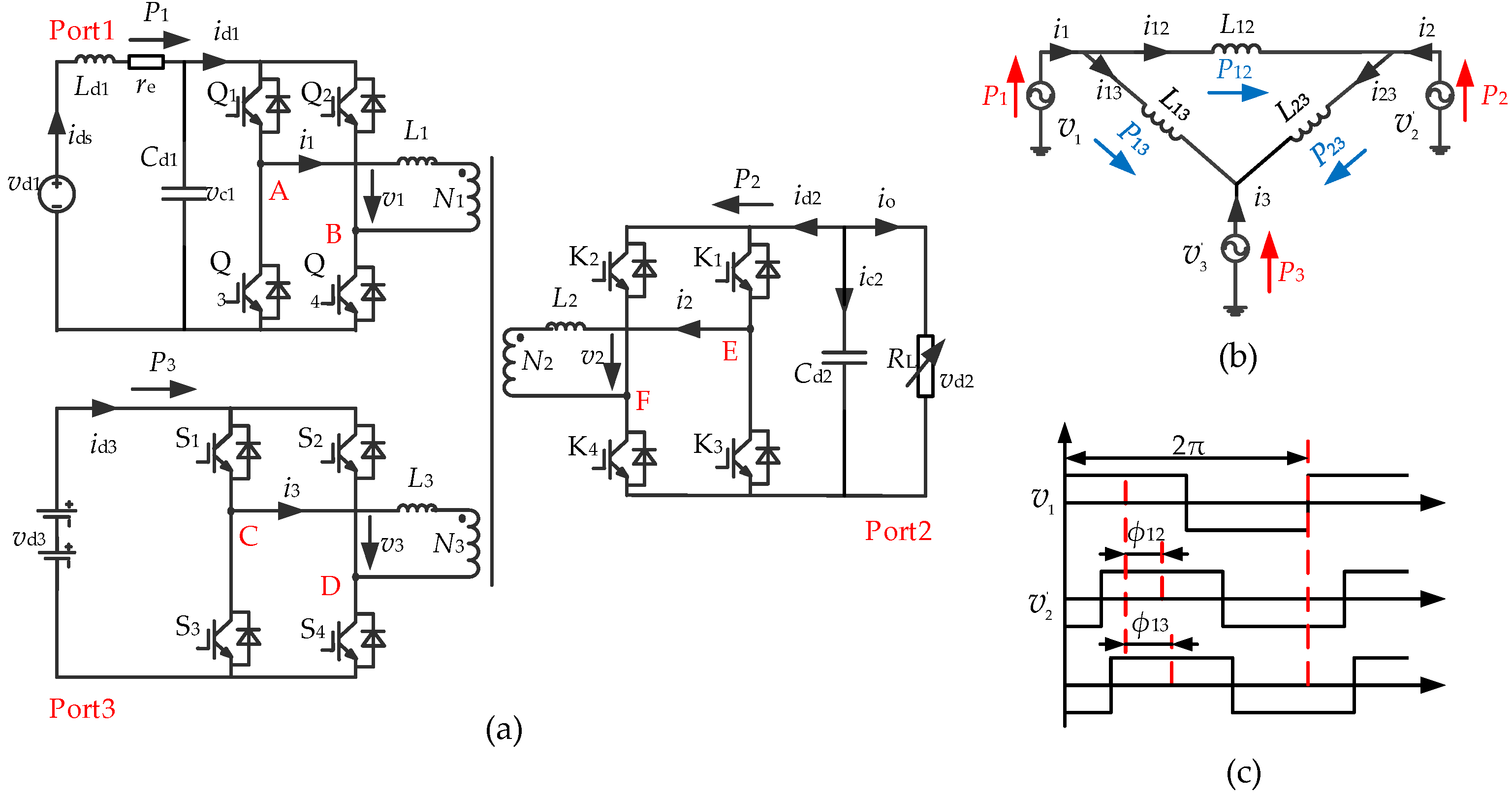
The circuit topology of an isolated TPC is presented in Figure 1a. In this figure, a DC power supply (e.g., it can be a fuel cell or a photovoltaic cell) is set in Port 1, and the power supply, vd1 is connected in series with an inductor Ld1, and re represents the equivalent series resistance (ESR) of Ld1. There is 180° phase shift between leg A and leg B, and the duty cycles of all switches in Port 1 are set to be 50% and the drive signals of the switches on the same leg are complementary. The Port 2 and Port 3 are connected with load and energy storage (ES) respectively and their switching patterns are as same as the switching mode of Port 1. A simplified equivalent Δ-connected circuit of the TPC by transferring the related parameters of Port 2 and Port 3 to Port 1 is given in Figure 1b. If the voltage between the middle points of leg A and leg B, v1 is defined as a reference, the phase shifts of v2 and v3 relative to v1 are denoted as ϕ12 and ϕ13 respectively, and they are shown in Figure 1c. Moreover, L1, L2, and L3 are equivalent series inductances (including winding leakage inductance and additional inductance) of the three transformer windings. The expressions of L12, L13, and L23 of the Δ-connected circuit shown in Figure 1b are defined by (1).
and are expressed by (2).
In each switching cycle, the total power transmitted between any two ports is approximated to its fundamental component. Therefore, the Fourier expansion based fundamental component analysis method is employed for theoretical analysis in this study. By utilizing the equivalent Δ-connection circuit in Figure 1b, the power equations of each port can be written as in (3).
where
In (4), Vd1, Vd2, and Vd3 are the rated amplitudes of v1, v2, and v3, N1, N2, and N3 are the transformer winding turns of respective ports, and ωs is the switching angular frequency. Since the summation of P1, P2 and P3 is kept at zero as shown in (3), that means the power of one port can be determined using the powers of the other two ports. From this point of view, the energy storage port is usually taken as an energy buffer that can be charged or discharged determined by the power delivery and load conditions of Port 1 and Port 2 respectively. According to (3) and (4), the power of Port 1 and Port 2 can be formulated as (5) and (6) respectively.
Therefore, the corresponding average currents in each switching cycle can be derived as (7) and (8) respectively.
By applying partial differential operation in (7) and (8) respectively, (9) can be obtained for a steady-state operating point A (ϕ120, ϕ130).
Consequently, (9) can be simplified as (10).
As shown in (9), besides the circuit parameters, the value of any matrix element in GA, Gxy (x = 1, 2 and y = 1, 2) is determined by the steady-state parameters (ϕ120 and ϕ130). And it can be also seen from (10) that there are couplings between and caused by and .
The small signal linearization model of the three-port converter can be derived as in (11) by applying KCL and KVL laws in Figure 1.
3. Control Strategy for TPC
3.1. Decoupling Control for TPC
Assuming the matrix, GA given in (10) can be simplified to a diagonal matrix given in (12) by introducing a decoupling matrix H defined in (13).
The decoupling control block diagram is presented in Figure 2. In this figure, Gv and Gc represent the voltage controller and current controller respectively, which can be synthesized by using Bode plot based design method in frequency domain. In Figure 2, the open loop transfer functions of the voltage and current control subsystems are Gvo = G11G1 and Gco = G22G2 respectively, the transfer functions of G1 and G2 are given in (14). The resonant angular frequency of G2 is .
3.2. Virtual Damping Method
For Port 1 in Figure 1, Ld1 and Cd1 are utilized to constitute an LC filter to limit the amplitude of the double-switching frequency component of ids and reduce the negative impact of high-frequency ripple current on the power source (e.g., a fuel cell). However, this might cause performance degradation or an instability issue in current control subsystem due to the high resonant peak and a very weak damping ratio introduced by a pure LC circuit (re = 0) or with a very small value of re shown in (14). Though the resonant phenomenon can be addressed by decreasing the current control bandwidth, the dynamic performance cannot be guaranteed.
The block diagram of the current control subsystem, Gco = G22G2 is presented in Figure 3 according to (11). The transfer function, Hvr in Figure 2 is a compensation function that is proposed to implement virtual damping in this paper. The expression of Hvr is shown in Figure 3. In this figure, rv is the desired virtual resistor. If the output of Hvr, which is , is moved from the point A to the point B, then, Hvr in Figure 3 is changed to , and it makes Hvr a rational fraction. is used to attenuate the high frequency noise, and if the value of is high enough, then, becomes a resistor connected in series with , and the damping ratio of G2 becomes with the introduction of rv as a virtual resistor. In practical applications, the sampled ids is passed through Hvr, and then added to the output of the current controller to obtain the final phase shift between Port 1 and Port 3, and the value of can be selected between ωs and ωs/2.
3.3. LADRC for TPC
The small signal model shown in (11) can be transformed into two subsystems to implement the LADRC based control method. The two differential equations for current control subsystem and voltage control subsystem are given by (15) and (16) respectively.
In (15) and (16), and are taken as the output variables of the two subsystems, and are the control signals of the current control subsystem and the voltage control subsystem respectively.
is considered as an external disturbance of voltage control subsystem, while is considered as an external disturbance of the current control subsystem. Furthermore, fc and fv are used to represent the generalized disturbances that are associated with both inner and outer variable elements of the two subsystems (e.g., coupling, load, and operating point related parameter changes, etc.). In practical situations, the generalized disturbances, fc and fv are usually unknown and cannot be directly measured. Therefore, LESO is adopted to evaluate the generalized disturbances and relevant state variables in the LADRC method.
As for the current control subsystem, is selected as the state vector, the augmented state space model is formulated by (17)
where
The LESO of current control subsystem is constructed by (19).
where is the observed vector of . and Lc given in (20) is the observer gain that can be designed using the pole placement method [17].
where is the equivalent bandwidth of the observer.
It should be noted that the disturbance caused by the resonance of Ld1Cd1 circuit is included in the generalized disturbance, fc, therefore, the value of should be at least twice as large as , that means / should be satisfied to make the LESO obtain accurate value of fc, otherwise, the control performance might be significantly degraded.
Similarly, the LESO used for voltage control subsystem is presented in (21).
In (21), . is the output vector of (21) that corresponds to . And the coefficient matrix in (21) are given in (22).
The corresponding gain vector of the voltage LESO, Lv is shown in (23).
Assuming and can be observed accurately (), and if and in (15) and (16) can be expressed as (24).
The current and voltage control subsystems will be simplified to two simple cascaded integrators systems shown in (25).
The current and voltage control signals, uc and uv, for this cascaded integrator system can be proposed as (26).
where kpc, kpv, and kdc are controller parameters, and urc and urv are current and voltage reference signals, respectively. In (26), it can be seen that uc and uv represent equivalent PD (proportional-derivative) and P (proportional) controllers respectively. The closed-loop transfer functions of the current and voltage control subsystem can be formulated as (27) and (28) which are obtained by substituting the two equations in (26) into the two equations of (25) respectively.
In (27) and (28), and represent equivalent control bandwidths of the two closed-loop control subsystems with LADRC method, and is the equivalent damping of the current control subsystem, which should be designed to guarantee smooth current change in transient state process (there is no intense oscillations in dynamic process). It can be seen from (27) and (28) that steady state errors are eliminated in the current and voltage closed-loop control systems (when s = 0, unity gain is obtained in (27) and (28) respectively) by utilizing (26) as control law. Furthermore, the closed-loop control performances of the two subsystems are completely determined by the designed controller parameters (kpc, kpd and kpv) regardless of the changes of model parameters. This is a prominent characteristic of the LADRC method. , and , are the adjustable LADRC parameters in current and voltage control subsystems, respectively. Since LADRC method is observer based, the bandwidth of the observer should be kept sufficiently larger than the bandwidth of the control system to realize effective compensation. Therefore, the two ratios, / and / should be larger than two at least in practical applications to get accurate observed values [21], otherwise, the control performance might not be guaranteed.
4. Simulation and Experimental Results
4.1. Simulation Results
In order to verify the theoretical analysis and design results of the proposed method, a simulation model of the isolated TPC is developed by using MATLAB/Simulink, and the main parameters of the simulation model are listed in Table 1.
The steady-state operating point A (0.620, 0.379) is selected which corresponds to RL = 45 Ω, vd2 = 36 V and ids = 1.3 A, and an extra 0.2 Ω virtual resistor is introduced. The open loop transfer functions of the two subsystems are obtained by substituting the parameters listed in Table 1 into Gco and Gvo, respectively. The controllers Gc and Gv, given by (29), are designed for the decoupled current and voltage subsystems respectively by using the frequency domain design method.
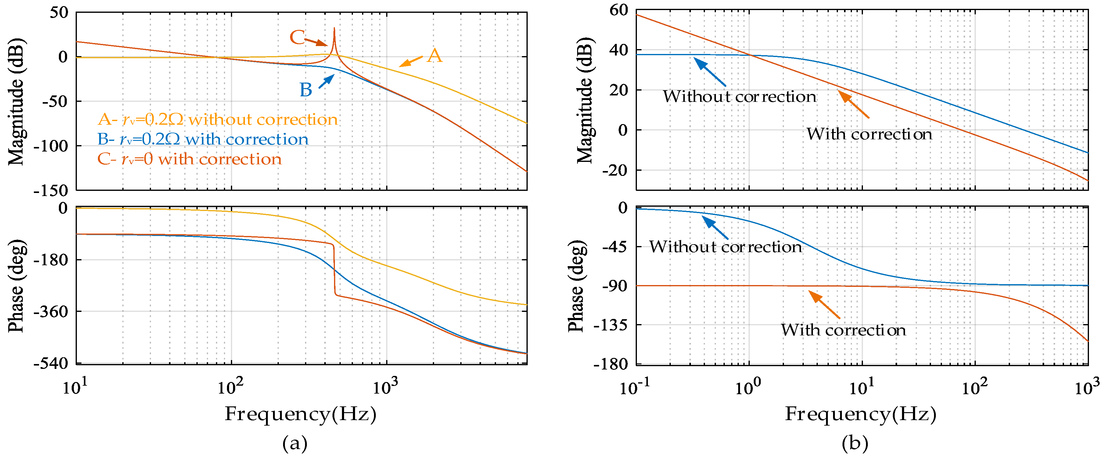
The Bode plots of the two subsystems with and without correction are shown in Figure 4a and Figure 4b, respectively.
As can be seen in Figure 4a, the crossover frequency of the corrected current control subsystem with rv = 0.2 (the curve B) is about 71 Hz, the phase margin is about 81°, and the gain margin is about 7 dB. The crossover frequency of the corrected voltage control subsystem is about 75 Hz, the phase margin is about 85°, and the gain margin is about 33 dB. As a comparison, if rv = 0.2 is cancelled, the corrected current control subsystem (the curve C) will be unstable, since the resonant peak (the corresponding angular frequency is ωn = 2887 rad/s) of the curve C will intersect with 0 dB axis under this condition.
For the control systems with LADRC method, the equivalent control bandwidths of the current and voltage subsystems are the same, (about 72 Hz) which are close to the designed crossover frequencies using the traditional frequency domain method. The observer bandwidths of the current and voltage subsystems are (about 660 Hz), and (about 318 Hz) respectively. The simulation results are shown in Figure 5.
Figure 5a shows simulation results of vd2 and ids with traditional frequency control under a step load change condition. As can be seen in Figure 5a, there is an obvious voltage drop (from 36 V to 35.2 V) at 0.5 s when the load is suddenly changed from 29 W to 52 W that resulted in transient fluctuations in ids (changed from 1.3 A to 1.25 A). When the load is suddenly reduced at 0.7s from 52 W to 29 W, current ids transiently increases from 1.3 A to 1.37 A, while vd2 increases to about 36.8 V, and then decreases gradually to its rated value after 100 ms.
The simulation results of the system with the LADRC method and rv = 0.2 Ω are shown in Figure 5b. In this figure, it can be seen that for the same load change, vd2 drops from 36 V to 35.6 V at 0.5 s when the load increased, and it increases from 36 V to 36.4 V at 0.7 s when the load decreases. However, current is changed slightly with respect to the load change. For instance, the current drops from 1.3 A to 1.28 A when the load reduced and it increases from 1.3 A to 1.32 A when the load is increased. By comparing the result shown in Figure 5, it can be seen that the amplitude of ids fluctuation in the system controlled with LADRC is lower than that of the system controlled with the traditional frequency control method. Also, the transient recovery time of vd2 is much shorter than that of the system with the traditional frequency control. These results imply that the information of the load change observed by LESO is effectively utilized in the control system.
4.2. Experimental Validation and Analysis
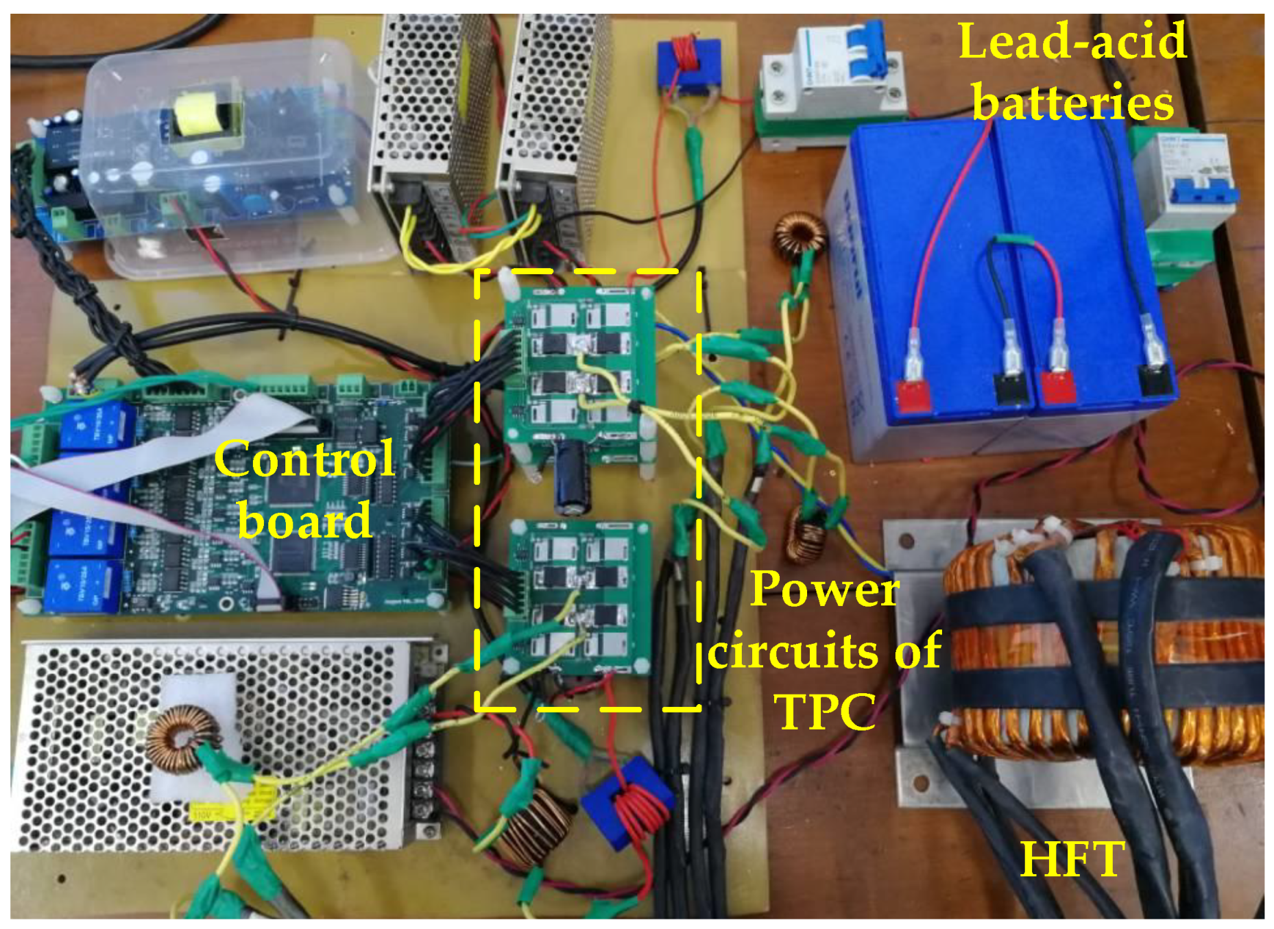
In order to further verify the effectiveness of the proposed method, an experimental platform was developed as shown in Figure 6. The circuit parameters and load change conditions of the experimental system are similar to the simulation model. The experimental results are shown in Figure 7, Figure 8, Figure 9, Figure 10 and Figure 11.
Figure 7 shows the experimental results, ids, vd2, Δvd2 (fluctuation of vd2) and io achieved for the developed converter controlled with the traditional frequency control method. The results of ids and Δvd2 (vd2 was controlled to 36 V) for a sudden load increase are shown in Figure 7a. As shown in this figure, there is about 0.24 A drop in ids and 0.8 V drop in vd2 when the load is suddenly changed from 29 W to 52 W. Figure 7b shows the current and voltage changes with respect to sudden load drop where the current and voltage are increased by about 0.24 A and 0.9 V respectively.
The effect of the proposed virtual resistor method on ids control is conducted by removing and re-adding the virtual resistor with the same current controller used in Figure 7. The experimental results are shown in Figure 8a, it can be seen that there are serious oscillations in ids (the current control subsystem is unstable in this case as indicated by the curve C in Figure 4 and voltage ripples (∆vd2) of vd2 are also increased with the same oscillation frequency of ids. While the virtual resistor scheme is re-performed, the oscillation of ids can be suppressed soon, and the amplitude of voltage ripple in vd2 becomes lower.
The experimental results of ids, vd2, Δvd2 and io with the LADRC method and rv = 0.2 Ω are shown in Figure 9. As shown in Figure 9a, when the same load increment (23 W) is experienced small changes are observed in ids (changes from 1.3 A to 1.35 A) and vd2 (changes from 36 V to 35.6 V) because of the coupling between current and voltage subsystems. As shown in Figure 9b, for a sudden load reduction, ids is changed from 1.3 A to 1.25 A, and vd2 is increased for about 0.5 V. Also, as illustrated in Figure 9, the fluctuations of ids and vd2 in the transient process with the LADRC method are lower than those with the traditional frequency control method as shown in Figure 7, and the voltage transient recovery time with the LADRC method is much shorter than that with the traditional frequency control. These results indicate that the control system with the LADRC has better decoupling performance and adaptability to the operating point changes compared to the control system with the traditional frequency control.
The experimental result with and without 0.2 Ω virtual resistor with LADRC method and ωn = 2887 rad/s is presented in Figure 8b. As shown in this figure, there are obvious current oscillations in ids when rv = 0.2 Ω is removed, since the observer bandwidth () is not sufficiently higher than the resonant angular frequency of Ld1Cd1 circuit (). And it is similar to the case shown in Figure 8a, the current oscillations can be attenuated effectively if the virtual resistor method is reused.
For comparison study, the resonant angular frequency of G2(s) in (14) is reduced to ωn = 1521 rad/s (by setting Ld1 = 160 μH and Cd1 = 2700 μF), then there is no oscillations in ids as shown in Figure 10, that means ids can be controlled well since the ratio of / is about 2.73 which is larger than two in this case, it means that the impact caused by the resonance of Ld1Cd1 circuit can be much accurately observed by the LESO.
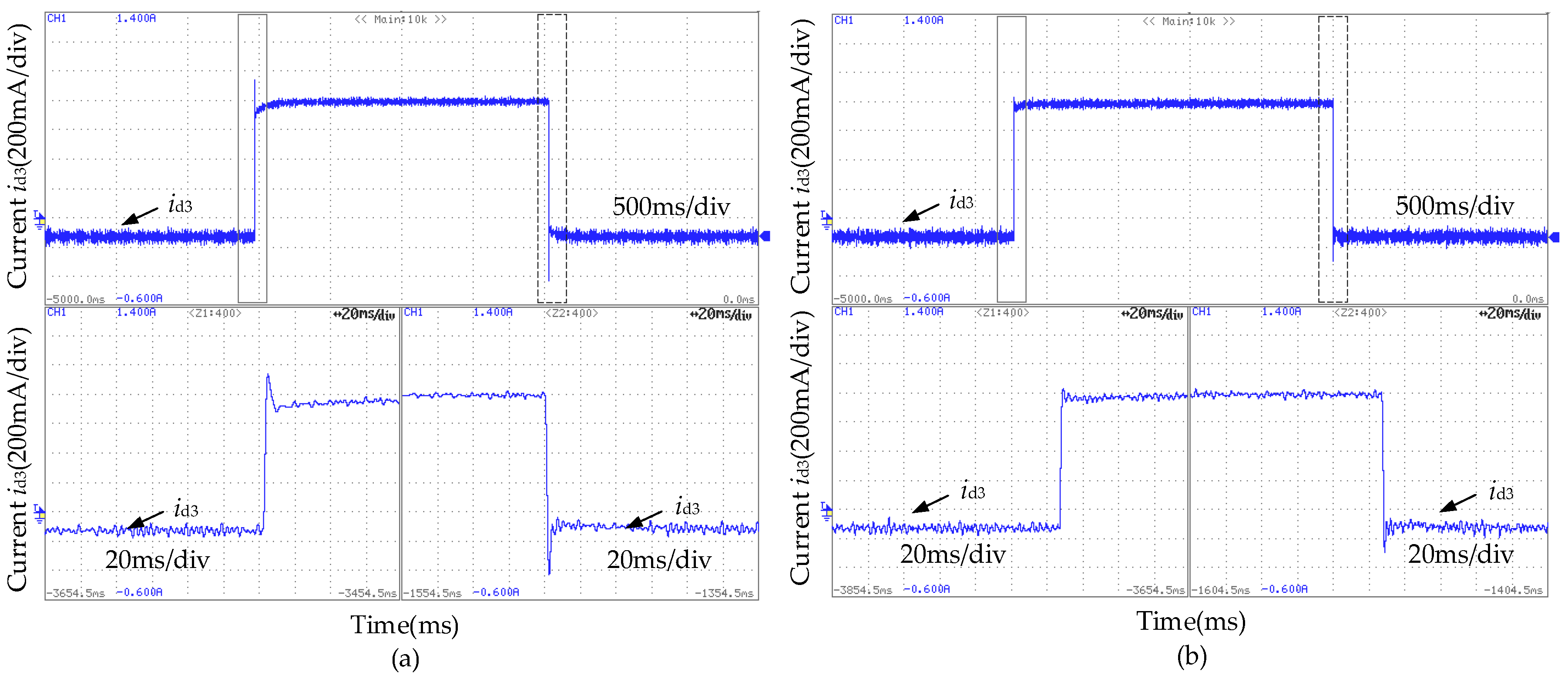
The battery current id3 for the traditional frequency control and LADRC are shown in Figure 11a and Figure 11b, respectively. In Figure 11, it can be seen that not only the overshoot of id3 with the LADRC is relatively lower, but also the transient recovery time of id3 is shorter than that obtained using the traditional frequency control. This indicates the LADRC method can provide better dynamic balance in the power delivery process. The results shown in Figure 11 have some internal relations with the experimental results presented in Figure 7 and Figure 9. For instance, compared to Figure 11b with LADRC method applied, the battery overshoot current, id3 shown in Figure 11a is larger when traditional frequency control method is applied. Larger overshoot current causes significant drop in ids shown in Figure 7a, whereas smaller overshoot of id3 shown in Figure 11b with LADRC resulted in much smaller overshoot in ids shown in Figure 9a.
5. Conclusions
The model parameter variation caused by the operating point changes and couplings between different ports during power delivery in an isolated three-port converter has a negative impact on the converter control performance. In this study, the LADRC method is employed to control the three-port converter. In the LADRC method, the possible model parameter uncertainties, load changes and the negative impact of LC circuit resonance are all expressed as a generalized disturbance that is considered as a state variable and observed by the LESO which is utilized to synthesize the control signal. In this method, the bandwidth of the LESO is sufficiently higher than the equivalent control bandwidth and the resonant frequency of LC circuit that guarantee the system dynamics and generalized disturbance can be accurately observed. Therefore, the desired closed-loop control performance that is independent of parameters changes and external disturbances can be obtained. And a virtual resistor based method is proposed to increase damping ratio of the current control subsystem of TPC which is beneficial to further improve current control performance using LADRC method. The simulation and experimental results revealed that the proposed method is robust against model parameter changes and external disturbances. Therefore, the dynamic control performance of the three-port converter can be improved significantly.
Author Contributions
Conceptualization, J.Y., M.L. and H.C.; Validation, M.L., J.Y. and H.C.; Writing-Original Draft Preparation, J.Y. and H.C.; Writing-Review & Editing, N.G., M.V. and M.L.
Funding
This work is sponsored by the National Natural Science Foundation of China (No.51479042 and No. 51761135013), and the fundamental research funds for the central universities of China (No. HEUCFG201822).
Conflicts of Interest
The authors declare no conflict of interest.
References
- Tao, H.; Kotsopoulos, A.; Duarte, J.L.; Hendrix, M.A.M. Design of a soft-switched three-port converter with DSP control for power flow management in hybrid fuel cell systems. In Proceedings of the 2005 European Conference on Power Electronics and Applications, Dresden, Germany, 11–14 September 2005. [Google Scholar]
- Tao, H.; Duarte, J.L.; Hendrix, M.A.M. A Distributed Fuel Cell Based Generation and Compensation System to Improve Power Quality. In Proceedings of the 2006 CES/IEEE 5th International Power Electronics and Motion Control Conference, Shanghai, China, 14–16 August 2006. [Google Scholar]
- Ling, Z.; Wang, H.; Yan, K.; Sun, Z. A new three-port bidirectional DC/DC converter for hybrid energy storage. In Proceedings of the 2015 IEEE 2nd International Future Energy Electronics Conference (IFEEC), Taipei, Taiwan, 1–4 November 2015. [Google Scholar]
- Tao, H.; Duarte, J.L.; Hendrix, M.A.M. Line-Interactive UPS Using a Fuel Cell as the Primary Source. IEEE Trans. Ind. Electron. 2008, 55, 3012–3021. [Google Scholar] [CrossRef]
- Wang, L.; Wang, Z.; Li, H. Optimized energy storage system design for a fuel cell vehicle using a novel phase shift and duty cycle control. In Proceedings of the 2009 IEEE Energy Conversion Congress and Exposition, San Jose, CA, USA, 20–24 September 2009. [Google Scholar]
- Kim, S.Y.; Song, H.S.; Nam, K. Idling Port Isolation Control of Three-Port Bidirectional Converter for EVs. IEEE Trans. Power Electron. 2012, 27, 2495–2506. [Google Scholar] [CrossRef]
- Jiang, Y.; Liu, F.; Ruan, X.; Wang, L. Optimal idling control strategy for three-port full-bridge converter. In Proceedings of the 2014 International Power Electronics Conference (IPEC-Hiroshima 2014—ECCE ASIA), Hiroshima, Japan, 18–21 May 2014. [Google Scholar]
- Ajami, A.; Asadi Shayan, P. Soft switching method for multiport DC/DC converters applicable in grid connected clean energy sources. IET Power Electron. 2015, 8, 1246–1254. [Google Scholar] [CrossRef]
- Tao, H.; Duarte, J.L.; Hendrix, M.A.M. Three-Port Triple-Half-Bridge Bidirectional Converter with Zero-Voltage Switching. IEEE Trans. Power Electron. 2008, 23, 782–792. [Google Scholar] [CrossRef]
- Tao, H.; Kotsopoulos, A.; Duarte, J.L.; Hendrix, M.A.M. A Soft-Switched Three-Port Bidirectional Converter for Fuel Cell and Supercapacitor Applications. In Proceedings of the 2005 IEEE 36th Power Electronics Specialists Conference, Recife, Brazil, 12 June 2005. [Google Scholar]
- Zhao, C.; Kolar, J.W. A novel three-phase three-port UPS employing a single high-frequency isolation transformer. In Proceedings of the 2004 IEEE 35th Annual Power Electronics Specialists Conference, Aachen, Germany, 20–25 June 2004. [Google Scholar]
- Zhao, C.; Round, S.D.; Kolar, J.W. An Isolated Three-Port Bidirectional DC-DC Converter with Decoupled Power Flow Management. IEEE Trans. Power Electron. 2008, 23, 2443–2453. [Google Scholar] [CrossRef]
- Tao, H.; Kotsopoulos, A.; Duarte, J.L.; Hendrix, M.A.M. Transformer-Coupled Multiport ZVS Bidirectional DC–DC Converter with Wide Input Range. IEEE Trans. Power Electron. 2008, 23, 771–781. [Google Scholar] [CrossRef]
- Wang, L.; Wang, Z.; Li, H. Asymmetrical Duty Cycle Control and Decoupled Power Flow Design of a Three-port Bidirectional DC-DC Converter for Fuel Cell Vehicle Application. IEEE Trans. Power Electron. 2012, 27, 891–904. [Google Scholar] [CrossRef]
- Falcones, S.; Ayyanar, R. LQR control of a quad-active-bridge converter for renewable integration. In Proceedings of the 2016 IEEE Ecuador Technical Chapters Meeting (ETCM), Guayaquil, Ecuador, 12–14 October 2016. [Google Scholar]
- Gao, Z. Active disturbance rejection control: From an enduring idea to an emerging technology. In Proceedings of the 2015 10th International Workshop on Robot Motion and Control (RoMoCo), Poznan, Poland, 24 August 2015. [Google Scholar]
- Gao, Z. Scaling and bandwidth-parameterization based controller tuning. In Proceedings of the 2003 American Control Conference, Denver, CO, USA, 4–6 June 2003. [Google Scholar]
- Wang, W.; Gao, Z. A comparison study of advanced state observer design techniques. In Proceedings of the 2003 American Control Conference, Denver, CO, USA, 4–6 June 2003. [Google Scholar]
- Miklosovic, R.; Radke, A.; Gao, Z. Discrete implementation and generalization of the extended state observer. In Proceedings of the 2006 American Control Conference, Minneapolis, MN, USA, 14–16 June 2006. [Google Scholar]
- Sun, B.; Gao, Z. A DSP-based active disturbance rejection control design for a 1-kW H-bridge DC-DC power converter. IEEE Trans. Ind. Electron. 2005, 52, 1271–1277. [Google Scholar] [CrossRef]
- Zhu, B. Introduction of Active Disturbance Rejection Control, 1st ed.; Beihang University Press: Beijing, China, 2017; pp. 42–45. [Google Scholar]
Figure 1.
The isolated three-port converter: (a) topology; (b) equivalent Δ-connected circuit; (c) modulation scheme.
Figure 1.
The isolated three-port converter: (a) topology; (b) equivalent Δ-connected circuit; (c) modulation scheme.

Figure 2.
Decoupling control scheme of a three-port converter.
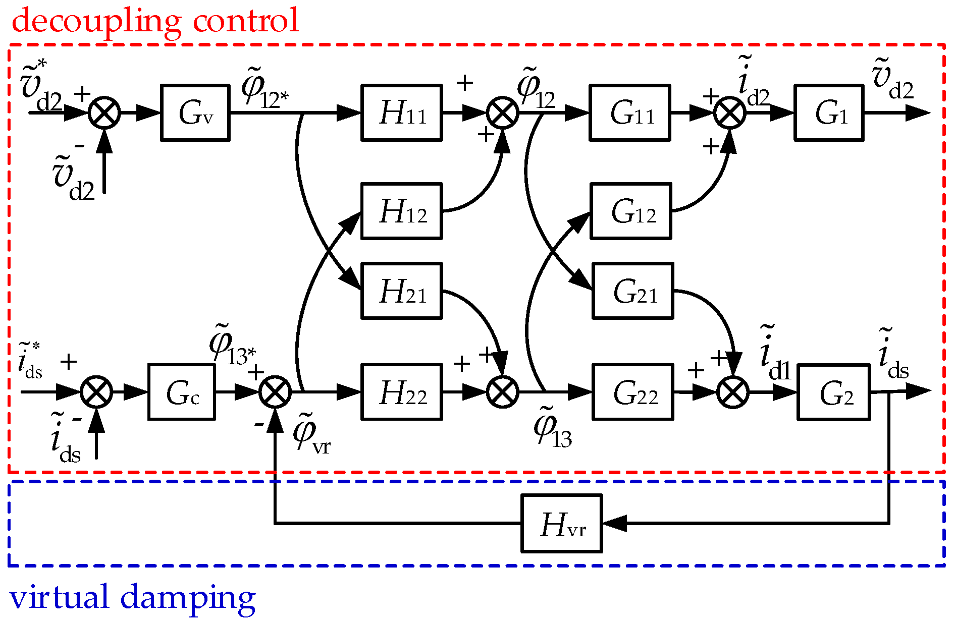
Figure 3.
Schematic diagram of virtual damping implementation.
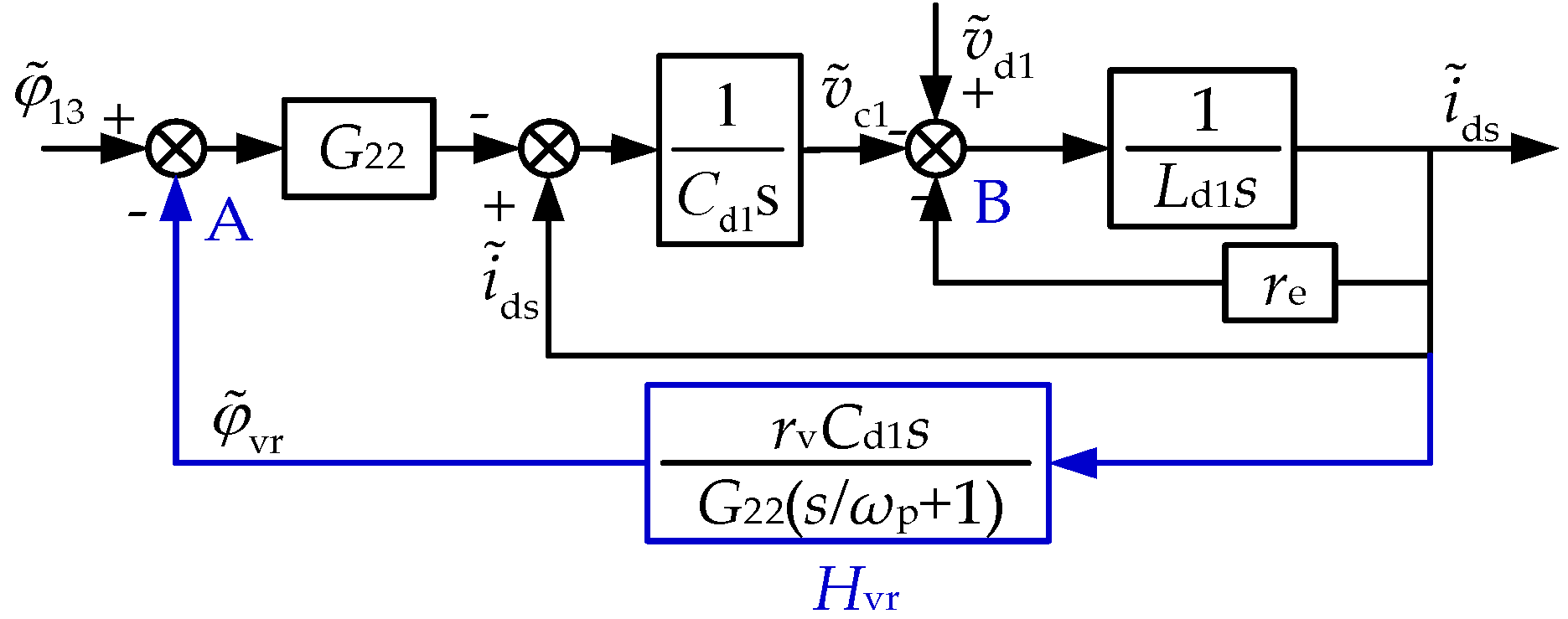
Figure 4.
The bode plots of subsystems by using traditional frequency control method: (a) ids subsystem; (b) vd2 subsystem.
Figure 4.
The bode plots of subsystems by using traditional frequency control method: (a) ids subsystem; (b) vd2 subsystem.

Figure 5.
The simulation results of the system: (a) with traditional frequency control method; (b) with the LADRC method.
Figure 5.
The simulation results of the system: (a) with traditional frequency control method; (b) with the LADRC method.
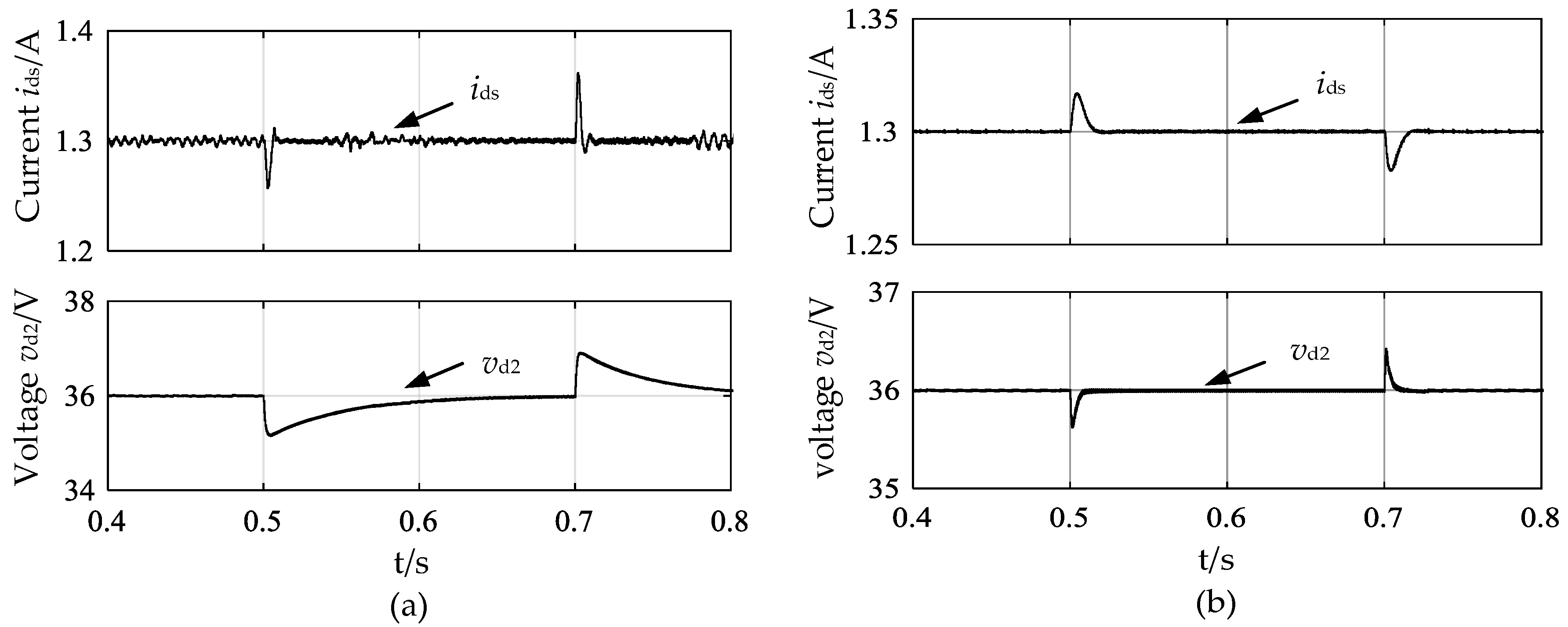
Figure 6.
Hardware experiment circuit of the three-port converter.

Figure 7.
The experiment results of ids, vd2, Δvd2 and io with the traditional frequency control method and rv = 0.2 Ω: (a) sudden load increase; (b) sudden load decrease.
Figure 7.
The experiment results of ids, vd2, Δvd2 and io with the traditional frequency control method and rv = 0.2 Ω: (a) sudden load increase; (b) sudden load decrease.
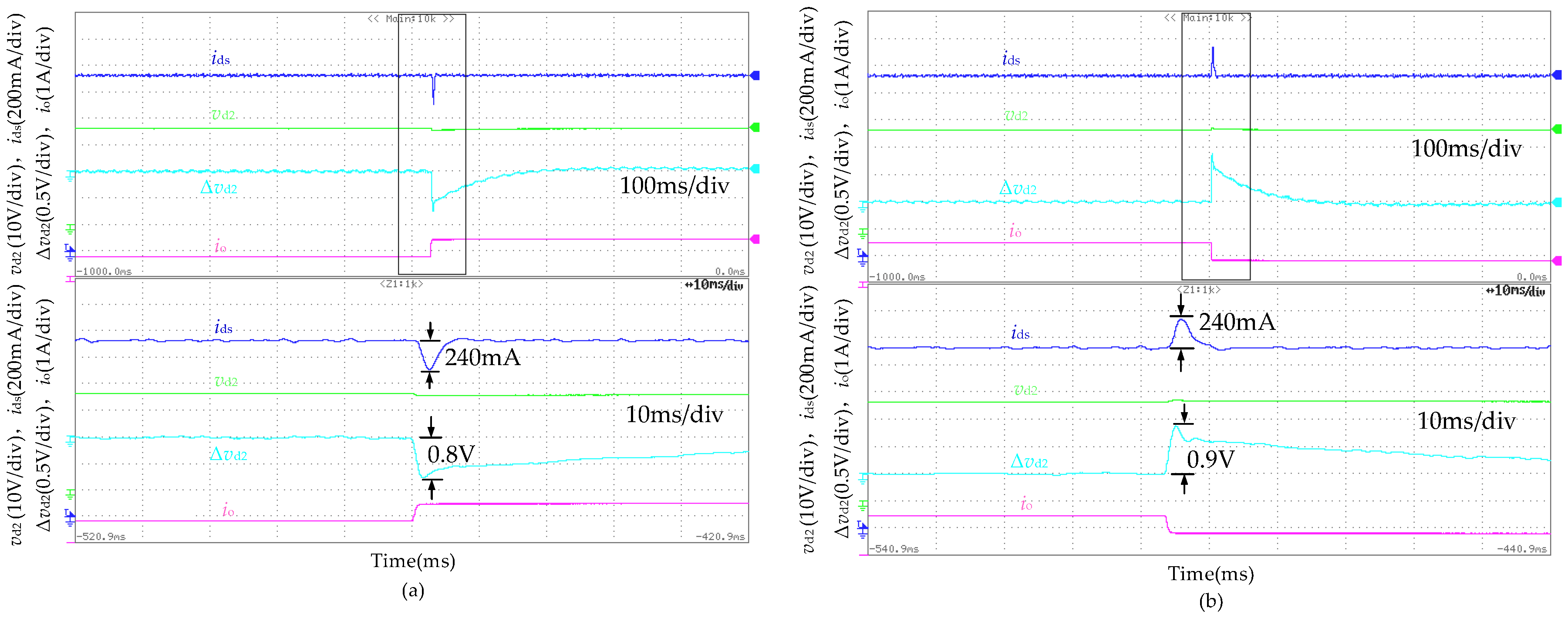
Figure 8.
The experimental results with and without rv = 0.2 Ω virtual resistor (ωn = 2887 rad/s): (a) traditional frequency control; (b) LADRC.
Figure 8.
The experimental results with and without rv = 0.2 Ω virtual resistor (ωn = 2887 rad/s): (a) traditional frequency control; (b) LADRC.
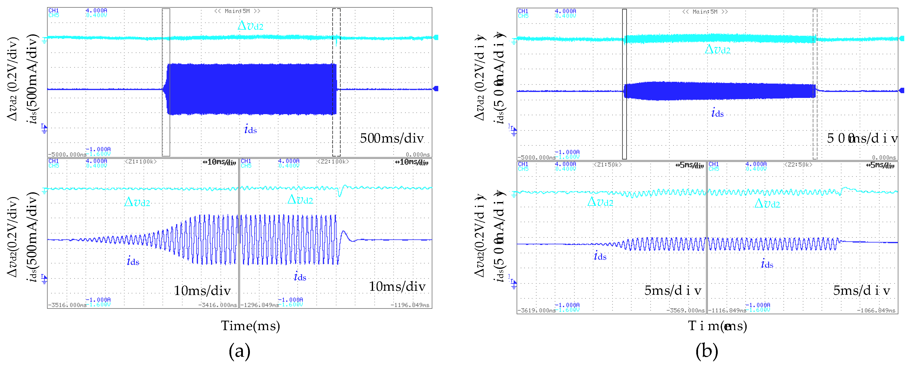
Figure 9.
The experimental results of ids, vd2, Δvd2 and io with LADRC method, ωn = 2887 rad/s and rv = 0.2 Ω: (a) sudden load increase; (b) sudden load decrease.
Figure 9.
The experimental results of ids, vd2, Δvd2 and io with LADRC method, ωn = 2887 rad/s and rv = 0.2 Ω: (a) sudden load increase; (b) sudden load decrease.

Figure 10.
The experimental results of ids, vd2, Δvd2 and io with LADRC method, ωn = 1521 rad/s and rv = 0 Ω: (a) sudden load increase; (b) sudden load decrease.
Figure 10.
The experimental results of ids, vd2, Δvd2 and io with LADRC method, ωn = 1521 rad/s and rv = 0 Ω: (a) sudden load increase; (b) sudden load decrease.
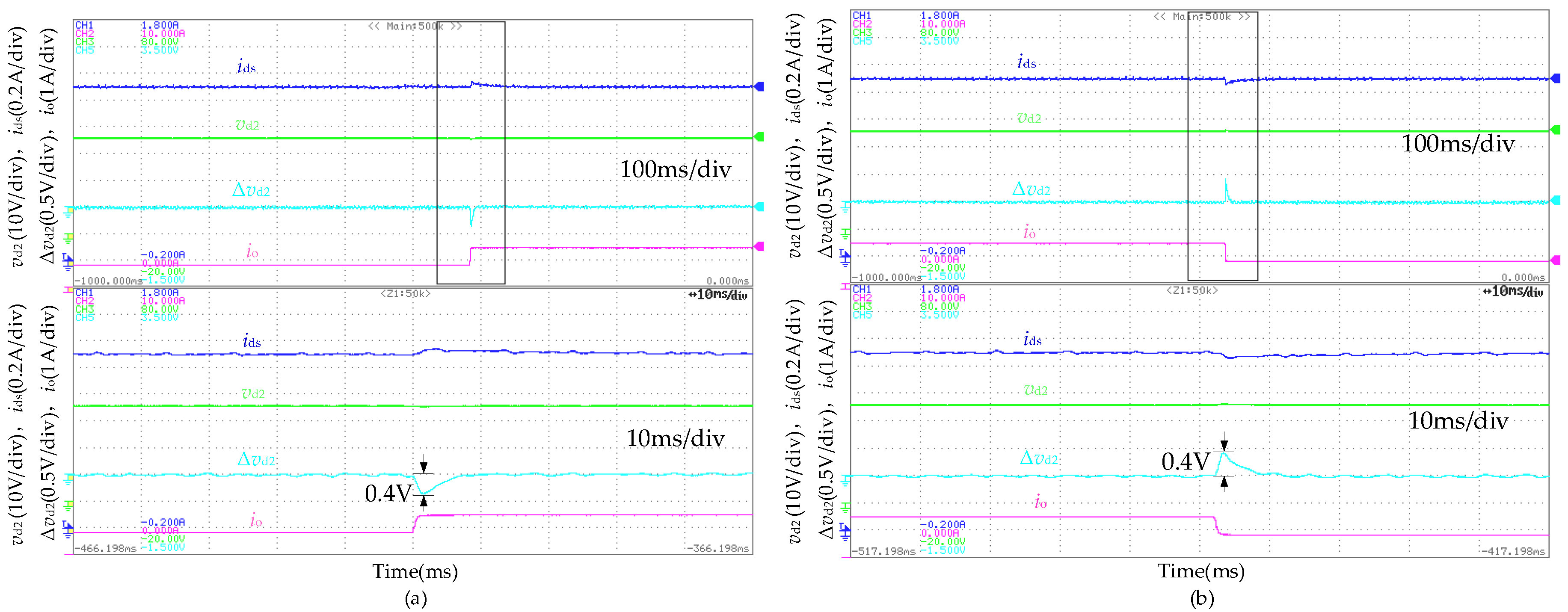
Figure 11.
The experimental results of battery current id3: (a) traditional frequency control; (b) LADRC.
Figure 11.
The experimental results of battery current id3: (a) traditional frequency control; (b) LADRC.

Table 1.
Parameters of The Simulation Model.
| Symbol | Name | Value |
|---|---|---|
| vd1 | DC input voltage | 24 V |
| vd2 | Output voltage | 36 V |
| vd3 | Battery voltage | 24 V |
| Ld1 | Input filter inductor | 100 μH |
| re | Input filter inductor ESR | 0.1 Ω |
| Cd1 | Input filter capacitor | 1200 μF |
| Cd2 | Output filter capacitor | 1000 μF |
| RL | Load resistor | 45 Ω/22 Ω |
| fs | Switching frequency | 20 kHz |
© 2018 by the authors. Licensee MDPI, Basel, Switzerland. This article is an open access article distributed under the terms and conditions of the Creative Commons Attribution (CC BY) license (http://creativecommons.org/licenses/by/4.0/).
Share and Cite
MDPI and ACS Style
You, J.; Liao, M.; Chen, H.; Ghasemi, N.; Vilathgamuwa, M. Disturbance Rejection Control Method for Isolated Three-Port Converter with Virtual Damping. Energies 2018, 11, 3204. https://doi.org/10.3390/en11113204
AMA Style
You J, Liao M, Chen H, Ghasemi N, Vilathgamuwa M. Disturbance Rejection Control Method for Isolated Three-Port Converter with Virtual Damping. Energies. 2018; 11(11):3204. https://doi.org/10.3390/en11113204
Chicago/Turabian StyleYou, Jiang, Mengyan Liao, Hailong Chen, Negareh Ghasemi, and Mahinda Vilathgamuwa. 2018. "Disturbance Rejection Control Method for Isolated Three-Port Converter with Virtual Damping" Energies 11, no. 11: 3204. https://doi.org/10.3390/en11113204
Note that from the first issue of 2016, this journal uses article numbers instead of page numbers. See further details here.