Electrical Modelling of a DC Railway System with Multiple Trains ^†

Abstract

Electrical modelling of rail tracks with multiple running trains is complex due to the difficulties in solving the power flow. The train positions, speed and acceleration are constantly varying resulting in a nonlinear system. In this work, a method is proposed for modelling DC electric railways to support power flow analysis of a simulated metro train service. The method exploits the MathWorks simulation tool Simscape, using it to model the mechanical and electrical characteristics of the rail track system. The model can be simulated to provide voltages at any position in the track and additionally, the voltages seen by any train. The model includes regenerative braking on trains, this is demonstrated to cause overvoltage in the feeding line if it is higher than the power demand of the other trains at that time. Braking resistors are used to protect the network from overvoltage by burning the excess energy. Through the implementation of Energy Storage Systems (ESSs), it will be possible to improve the energy efficiency and remove timetabling restrictions of electric railways by effectively controlling the rail track voltage. The paper proposes several methods to validate the model.

1. Introduction

Railways have been used in transportation since the beginning of the 19th century before they began to be electrified to transport passengers at the end of the same century. For many years now, there has been a demand to move from diesel trains to electric trains in order to reduce harmful emissions and noise and to take advantage of lighter-weight locomotives. Diesel-powered trains suffer from a decline in diesel supply and rising prices, due to its use in other transport modes, like cars and planes. Electric trains are cost effective because of their lightweight, which requires less energy for traction. In contrast, diesel-powered trains use high amounts of energy for traction due to their heavyweight, which is a result of the onboard energy sources. In the last few decades, the power demand of electric railways for freight and passenger transport has increased due to the need for effective and quiet transportation systems.

Electric railways can be powered by AC or DC voltage. The preference for AC or DC traction motors is based on safety, efficiency and economic benefits. Historically, DC was preferred for the ease of controlling trains’ DC motors. Economically, AC power traction is preferred for its ability to step up and step down the voltage, which reduces conductor size. DC cables are more expensive than AC cables, as a large diameter is needed to carry large DC currents.

High-voltage electric railways increase the distance between the feeding substations and decrease their number. In high-voltage electric railways, it is not preferable to use DC because of the difficulties in breaking fault currents. However, AC railways are not always more economical than DC railways. The impedance of the electric cables is higher in AC-electrified railways than in DC systems due to the skin effect and loop inductance. High impedance will cause a high voltage drop through the line, which requires more substations with a shorter distance between them in the case of low voltage rail systems. Consequently, low-voltage DC electric railways have fewer substations compared to AC, due to the smaller line voltage drop. Therefore, in low-voltage electrified railways, DC is preferred because it is more economical than AC.

In the UK, DC railway systems use overhead transmission lines and a 3rd rail or 4th rail. Overhead transmission lines were first introduced into electric railways in 1881 at the International Exposition of Electricity in Paris by Werner von Siemens. The 3rd rails were first used in Berlin Industrial Exposition in 1879 by installing them between the running rails. The 3rd rail was introduced in London in 1890. Overhead transmission lines are not commonly used in urban areas because they are challenging to build in confined spaces, such as tunnels and are not aesthetically desirable. The 3rd and 4th rails are placed on the ground close to the running rails. The main advantages of 3rd and 4th rail lines are the low price of construction, low cost of maintenance and the ability to construct them where space is limited. Moreover, they do not require expensive civil works for existing infrastructure, as in overhead lines. However, overhead lines are safer due to reducing the possibility of electrocution [1,2,3,4].

Substations provide the power from the AC electrical grid through DC rectification, whereby either 750 V or 1500 V is typically used in the UK. In some DC rail systems, running rails are responsible for carrying the return current to the substations through the connection between the train’s wheels and the rails. Only one feeder conductor is required in this case and is called the 3rd rail, set either beside the rails or between them. The currents pass through the running rails and create destructive arcing. However, currents might sneak through rails to the ground and return to the substations from different paths. These currents are called stray currents and they cause corrosion to the rails. Usually, corrosion occurs at the locations where the stray currents leave the running rails or re-join them.

In order to avoid damage to the railway track, a 4th rail is commonly used. In this case, the rail track has two running rails and two power rails, whereby the live (3rd) rail is placed on the side of the running rails. The return rail, which is the 4th rail, is placed in the centre, or on the other side of the track. The 4th rail is applied as a return conductor to substations to avoid using the running rails to pass the current, as this has been shown to cause premature erosion. A train is connected to the 3rd and 4th rails through a contact shoe. While in the previously used designs, the contact shoe touched the live rails at the top, it presently touches the live rails at the sides or from underneath to prevent accidents as well as protect live rails from adverse weather conditions [5,6].

In urban densely populated environments, the 4th rail track system is commonly used and there is typically a very short distance between passenger stations. As a result of this design, trains need to accelerate and decelerate rapidly in order to achieve top speeds. Therefore, lightweight vehicles travelling at low speed are favoured due to their ability to accelerate and decelerate across short distances. In braking, traction motors transform into generators, whereby traction currents are reversed and redirected into the feeding lines to slow trains down. This results in high power generation before leaving a station, along with high power regeneration before reaching the next station [7]. This surge in power can cause voltage peaks and dips due to the resistance in the conductors and, as the substations are commonly just rectifiers, there is no power flow back to the grid.

Based on the IEEE standards, voltage is deemed normal if its value deviates by less than 10% of the nominal value. Conversely, a deviation above 10% that lasts between 0.5 and 30 cycles is called transient voltage. If the deviation exceeds 110% of the nominal value, it is denoted as voltage swell. Similarly, voltage sag occurs when the voltage deviation is in the 10–90% range. The appearance of voltage sags in the AC network is a severe issue since it propagates through the rectifier substations following nonlinear paths. This issue is well presented in Reference [8] and two methods are suggested for voltage sag measurements. Finally, if the voltage deviation is between 10% and 20% and lasts for more than 60 s, it is called over/under voltage.

The power that is regenerated on braking is ideally consumed by other trains on the same conductor rails. However, to protect the track from high voltages, this excess power is dissipated as heat through the onboard braking resistors. This energy is regarded as wasted, as it cannot be reused. Furthermore, the heat that is dissipated can increase the overall energy requirements for cooling the underground rail systems [9].

Empirical evidence and more recently with a number of pilots installed around the world indicates that, Energy Storage Systems (ESSs) could support peak powers on DC rail tracks, which will in turn increase the system efficiency. To study the ESS size, location and control, it is necessary to develop a sophisticated voltage model capable of supporting multiple train simulations.

The electrical configuration of the railway system is time variant based on the moving trains. The network variability and nonlinearity (due to the rectifier substations) make the system power flow analysis challenging. In extant studies, power flow in DC railways is usually modelled by adopting Gauss-Seidel, Newton-Raphson and current injection methods. Gauss-Seidel method is easy to implement but introduces convergence issues, whereas Newton-Raphson and current injection methods converge quickly. However, these methods require complex formulation for the corresponding Jacobian matrix. A new linear method based on a Jacobian approach that could be applied to solve electric railways power flow is proposed in Reference [10].

Kulworawanichpong [11] not only solved the power flow of a multi-train model but also avoided the complication that arises due to using derivatives within matrices by adopting a simplified Newton-Raphson method. The proposed method is efficient for use when multiple trains are operating on the same railway network due to the simulation time and calculation complexity reduction. In the conventional methods, the Jacobian matrix needs to be recalculated iteratively. However, when the simplified Newton-Raphson method is adopted, the off-diagonal elements are only calculated once and their values will remain fixed while the diagonal elements are recalculated at every iteration.

Mohamed, Arboleya and Gonzalez-Moran [12] proposed a method for solving the electric railway power flow in DC traction, which they denoted as a Modified Current Injection (MCI) method. This method is a modification of existing algorithms, aiming primarily to improve the convergence and reduce the solving time. Moreover, MCI can be applied to solve the electric railway power flow, whether the substations are reversible or non-reversible. One of the drawbacks of this method stems from the need to provide the initial voltage profiles for the nodes in order to calculate the currents injected into the nodes.

Jabr and Dzafic [13] solved the power flow of a DC railway with 144 running trains by using the current injection method, also known as the Conductance Matrix Iterative (CMI) method. This approach is beneficial, as it avoids overvoltage by adjusting the regenerative energy that is reinjected through to bi-directional substations. Furthermore, when the substations are non-bi-directional (rectification only), they are switched off and the regenerating trains are switched to voltage-current sources. The main objective of CMI is to reduce the number of required iterations, thus increasing the speed which the system solution is generated.

Different simulation methods for electric railways have been proposed in extant literature [14,15,16,17,18,19,20]. However, these approaches provide only the voltages experienced by the trains and not the track voltage. The authors of [9] suggested a simulation method that uses MATLAB Simulink to solve the power flow of an electric railway with seven substations. The proposed model measured the traction substations voltages and currents.

A single train running on the Sukhumvit Line was simulated by Mongkoldee, Leeton and Kulworawanichpong [21] to calculate the voltage at the train’s location, traction substations power and power losses in the transmission line. The system was modelled by a MATLAB M-file and the power flow was solved using the current injection method. Arboleya, Diaz and Coto [22] avoided the variation of the railway power network by using graph theory. Thereafter, simple matrix formulation was developed to solve the power flow. The proposed approach exhibited high accuracy compared to that of the commercial software DIgSILENT. Several railway simulation tools have been provided by the industry such as Vitas, Trainops, Sitras Sidytrac and TOM.

Simulating electric railways is essential to improve their performance. Simulation helps in selecting optimal storing technology, size, site and voltage control. Power flow analysis is essential for the planning and development of electric railways. Therefore, it is crucial to develop a simulation method that considers the features of modern electric railways. In this work, a simulation approach was developed for modelling the mechanical and electrical characteristics of a 4th rail track, including vehicles, rail track and substations. The electrical performance of the trains and their effects on each other’s behaviour were studied. The trains were assumed to be in motion, which can change the configuration and equations of the system at every time step. Consequently, the proposed simulation tool has to be receptive to these changes.

Before designing an electric railway model, it is important to consider the computational complexity associated with the system nonlinear characteristics and high temporal resolution. The primary purpose of this work was thus to develop a simulation method that can accurately analyse the power flow, as well as measure the track voltage and the voltages that the trains are subjected to. Consequently, onboard or stationary ESSs can be introduced into the model for analysis and optimisation.

2. Case Study

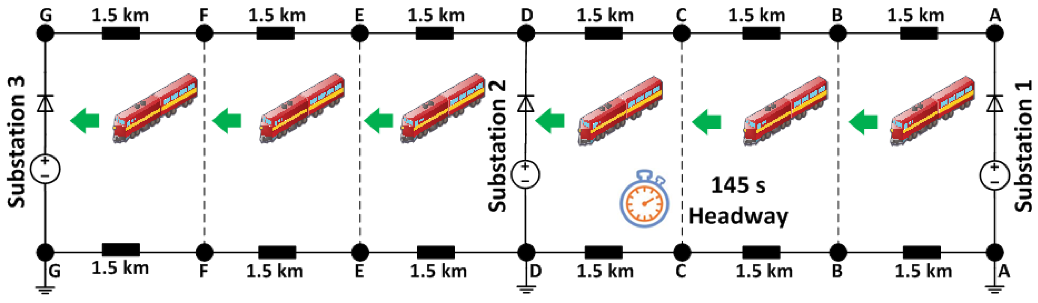
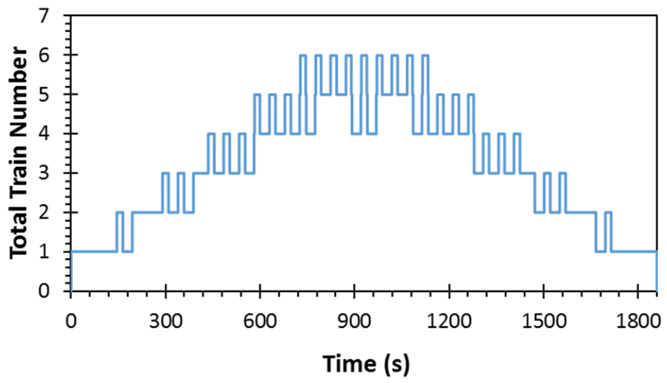
In the test scenario, equal distances between the rectifier substations and between the passenger stations are assumed. Figure 1 shows that trains are assumed to stop at seven passenger stations separated by 1.5 km. The total track length is 9 km and the three supply substations are staggered by 4.5 km. The railway line is divided into two electrical sections, which are not electrically coupled. In other words, if there are trains demanding power in the first electrical section, Substation 3 is not allowed to provide power to meet this load demand.

Six trains are modelled and are staggered by a time shift (known as headway) of 145 s. The trains start their journeys at Station A and finish their journeys at Station G. To demonstrate electrical validation, the journeys are repetitive and the characteristics and loads are the same for all trains. However, in order for the model to simulate realistic electric railways, real traffic scenarios need to be considered.

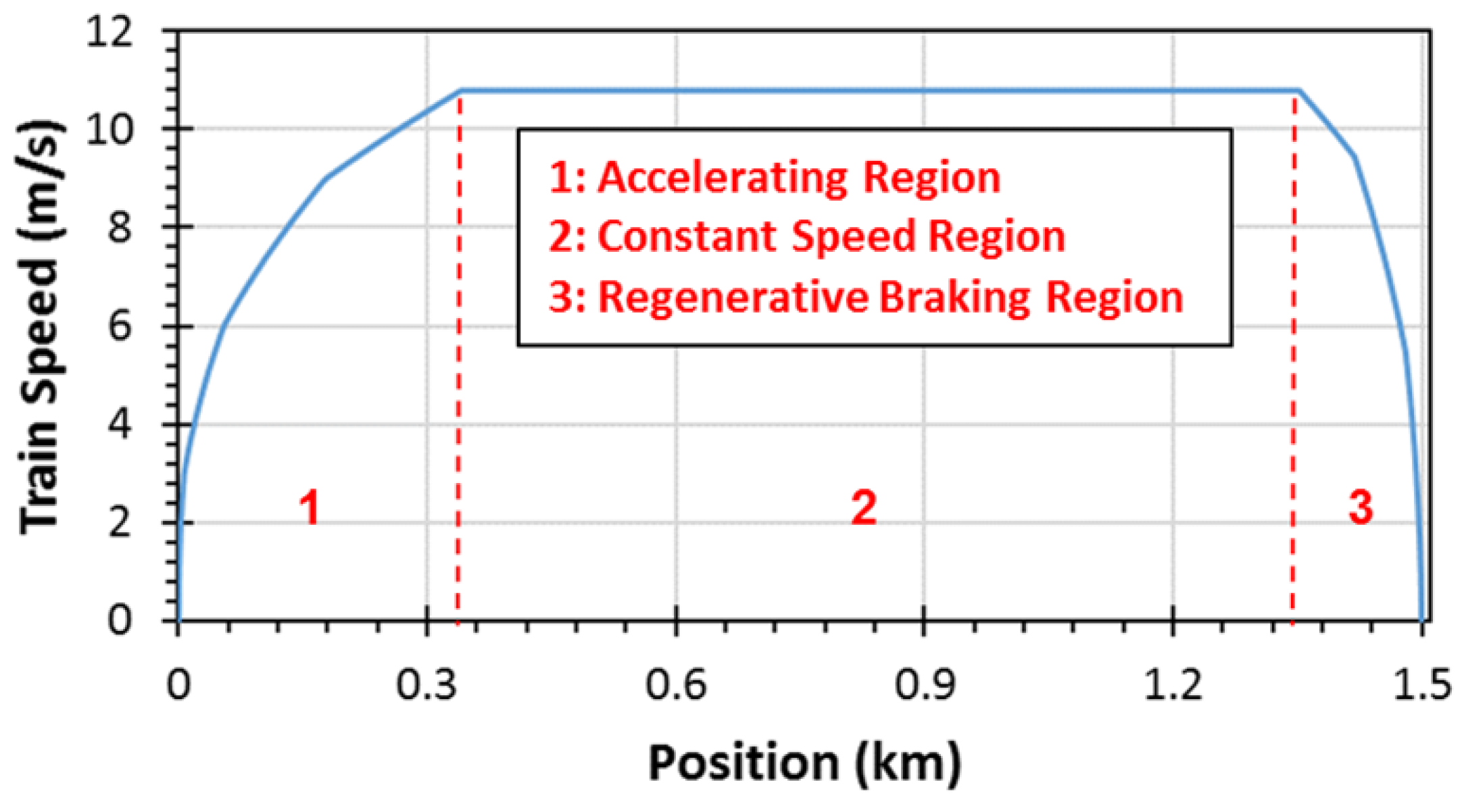
In practice, the trains’ weights change with the number of passengers onboard. However, in the case considered here, the trains have fixed weights, as it is assumed that they are fully occupied. The increase in the weight will increase the braking energy. Generally speaking, trains accelerate, cruise, coast and decelerate during their journeys. In the acceleration mode, the trains consume power from the railway traction system. In the cruising mode, the drawn power is constant, while in the coasting mode, the drawn power is almost zero. In the deceleration mode, the trains regenerate power to the railway traction system. Since the distance between the passenger stations is short in urban areas, the coasting mode was neglected in this case study. The typical speed profile of a train between any two virtual stations is shown in Figure 2, indicating that the maximum speed is 38.88 km/h. The six trains have the same speed profile that is repeated between any two consecutive passenger stations, with the mass of each train remaining the same.

It is assumed that the trains are restricted to a fixed timetable and their dwell time in the passenger stations is 30 s. Practically, the dwell time is variable due to its dependence on drivers’ behaviour and passenger loading and unloading time. The cyclic railway timetable was first used in 1931 in Netherlands for passengers’ convenience, by making the timetables easy to memorise. Later on, cyclic timetables were adopted by other European countries in their bus, metro and railway systems [23].

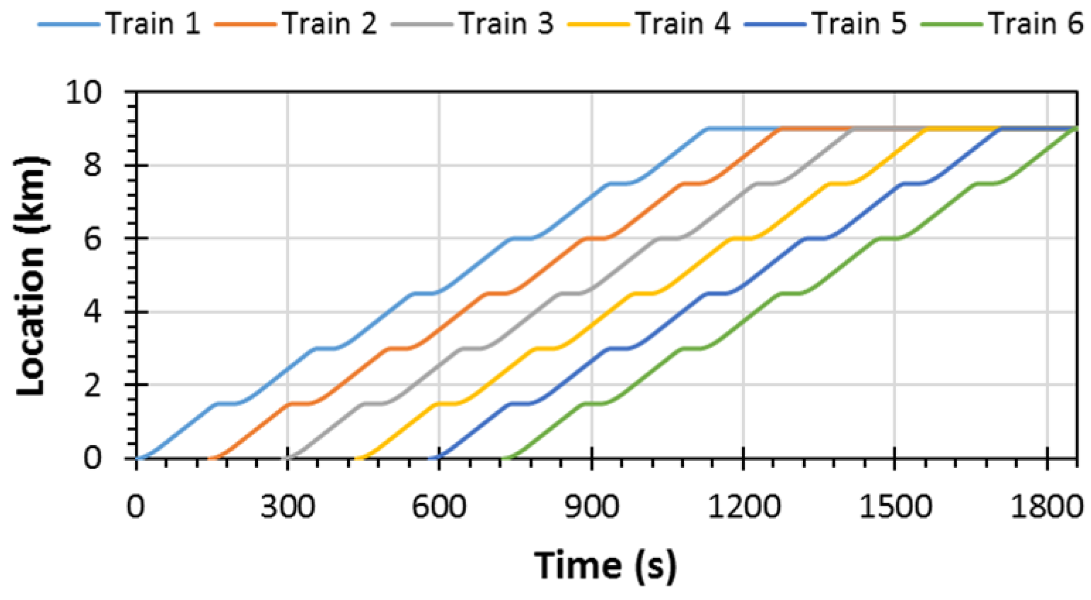
The train positions against time for the entire journey is shown in Figure 3. It can be seen that there is an overlap between the trains when one train is braking while another one is accelerating. This overlap plays a vital role concerning energy exchange and voltage stability. The greater the traffic density, the greater the energy exchange between the vehicles and the lower the dissipated energy. Consequently, it is expected to have more dissipated energy at the beginning and the end of the journey because the traffic density is not heavy.

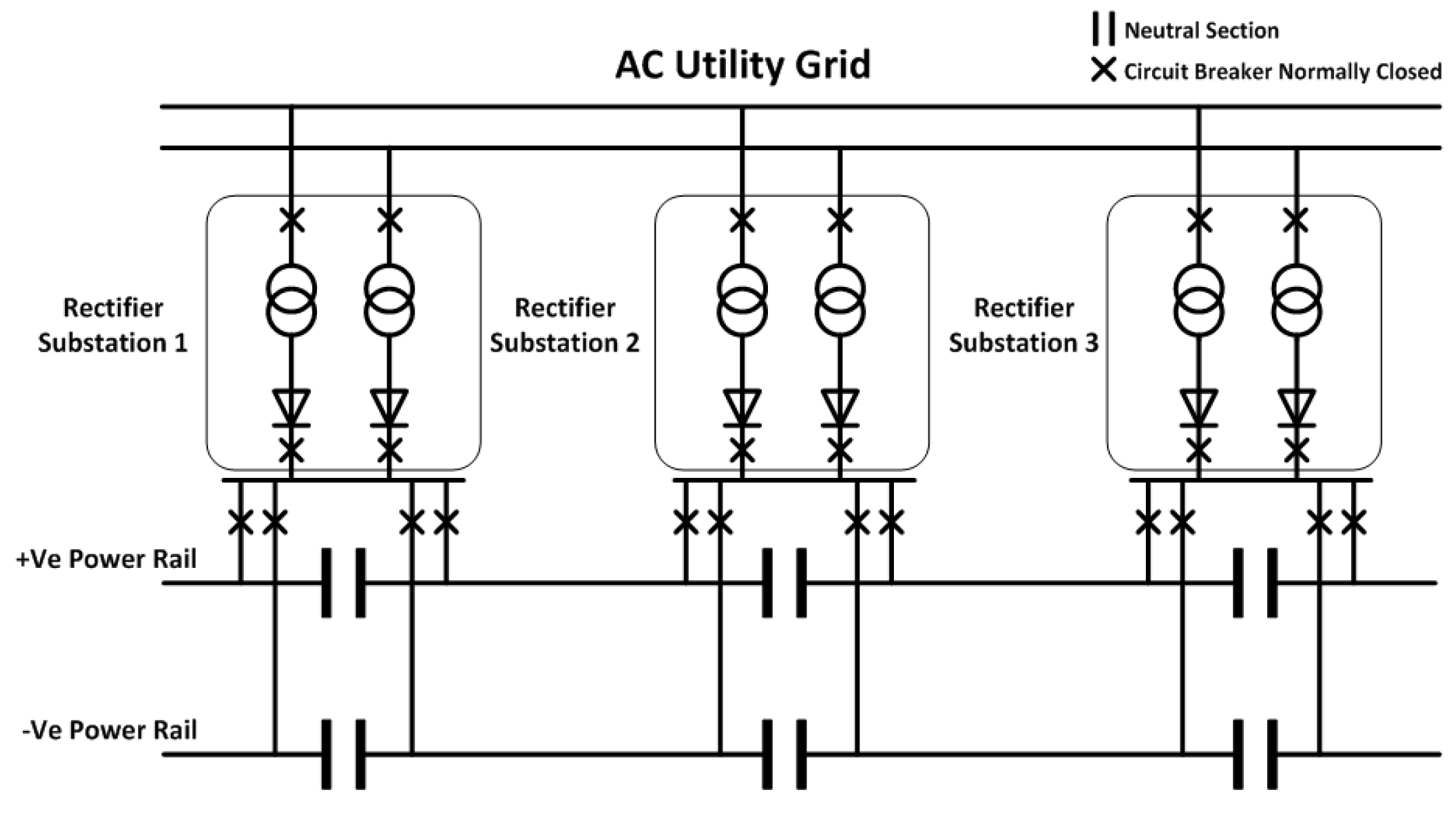
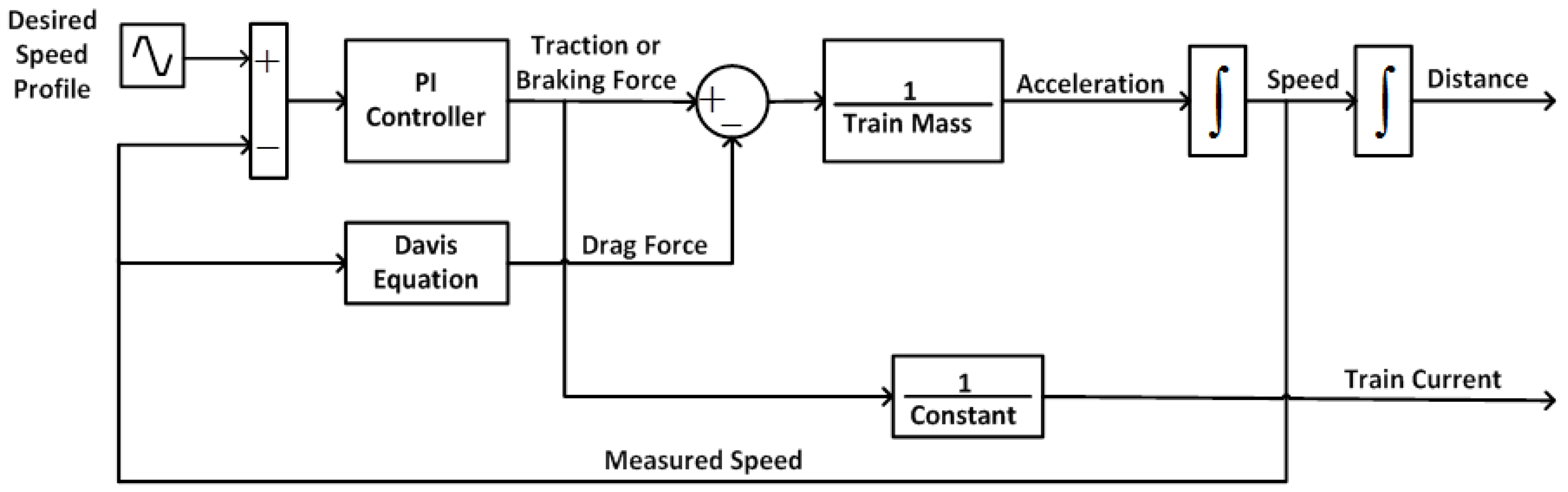
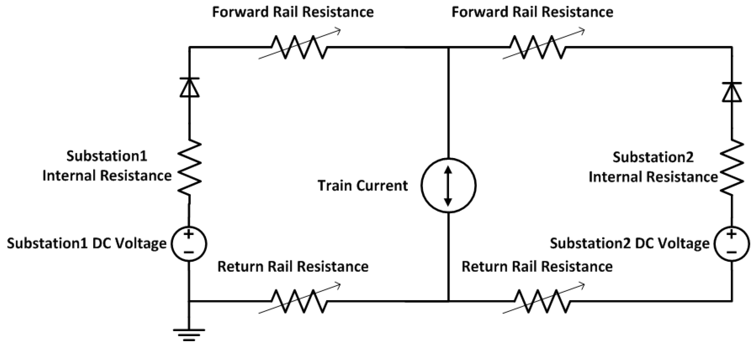
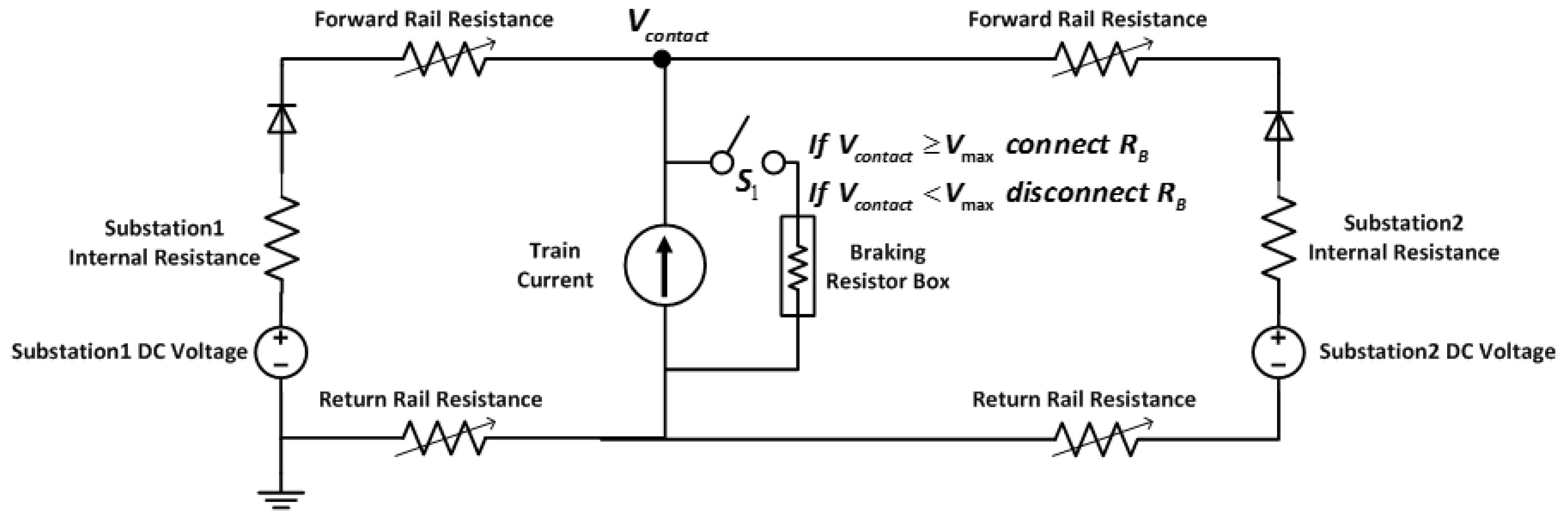
The traction system under consideration is shown in Figure 4. The substations are located at the specified locations and they include transformers and rectifiers. The transformers are responsible for stepping down the distribution network voltage. The rectifiers are responsible for converting the distribution network AC voltage into DC voltage. In each substation, there are two parallel rectifiers and transformers to increase the traction system reliability. The 3rd rail is responsible for conveying the electric power from the substations to the trains. The power returns to the substations through the 4th rail. The circuit breakers are normally closed to couple the rectifiers, which results in reducing the voltage drop. The two railway sections are electrically isolated by a dead zone, called neutral section, which is located at each substation. The train obtains power from the 3rd rail by continuous connection between its shoe and the 3rd rail. When the train reaches section gaps, the shoe is disconnected from the rail.

The DC railway system draws power from one of the national grid’s three phases. In that case, a significant imbalance occurs within the grid, which can be avoided by allowing adjacent substations to take power from different phases with the help of dead zones. These neutral sections are responsible for electrical isolation of railway sections. This sectioning is applied to balance the national grid by drawing power from different phases for adjacent substations. Thus, each rectifier substation is responsible for feeding two adjacent electrical sections only. The section is called double-end fed if it is supplied by two substations on its sides. When the section is supplied by one substation on one of its sides, it is called single-end fed. Trains should be coasting when they pass through neutral sections in order not to cause electric arcs. Another advantage of neutral sections is confining faults to one section, which increases the operational flexibility when lines are subjected to frequent traffic. Traction sectioning also permits maintenance to the traction substations without affecting the operation of the traction system.

3. Model Description

3.1. Vehicle Model

The train is represented by an ideal current source to reduce the calculation time and to simplify the complexity of representing the regenerative braking. The train is importing current when it is accelerating or cruising and is exporting current when it is decelerating. The train’s power demand changes with time due to the different speed modes, while the auxiliary power is always zero. For the sake of simplification, the efficiency of the traction power converters is ignored.

The length of the vehicle is ignored and each train is treated as a single point. The six modelled trains have the same current profile to enable electrical validation against repetitive journeys. The number of trains running on the track from the beginning until the end of the simulation is shown in Figure 5. During peak periods, the number of trains ranges from 4 to 6, reducing to 1–2 during the off-peak periods. In the middle of the simulation time, a very good power utilisation is expected due to high traffic. In contrast, the power losses in the braking resistors at the beginning and the end of the simulation are expected to be high due to low traffic. The time interval between each two consecutive trains is 145 s, which makes the power exchange good.

3.2. Traction Calculation

In order to move a train from its stationary state, a tractive force needs to be applied. The tractive force decreases when the train’s speed increases and depends on many factors, such as the vehicle weight, gradient, inclination and the trip time. Furthermore, the braking force is responsible for bringing the train to a standstill. While the train is moving the drag force, that consists of rolling resistance and air resistance, resists its movement. The traction force versus speed is limited to maximum train speed, the maximum traction force and the maximum power consumption. The equations used in this work to model the train dynamics are adopted from [24] as follows:

• The drag force $Q(v)$ in $kN$ is represented by the Davis equation:

  $$Q(v)=a+bv+c{v}^2.$$

  (1)

The coefficients of the Davis equation depend on the train type. When they are calculated experimentally, a represents the bearing resistance and is dependent to the vehicle mass, b represents the rolling resistance and c represents the air resistance. The values of the Davis coefficients are reported in

Table 1. Parameters of the Trains and the Electric Railway System.

Symbol	Quantity	Value
$m$	train mass	$27,215.5\mathrm{kg}$
$a$	Davis equation constant coefficient	$2.965\mathrm{N}$
$b$	Davis equation linear term coefficient	$0.23\mathrm{Ns}/\mathrm{m}$
$c$	Davis equation quadratic term coefficient	$0.005{\mathrm{Ns}}^2{/\mathrm{m}}^2$
$V_s$	substation dc voltage	$600\mathrm{V}$
$R_s$	substation inner resistance	$20\mathrm{m}\mathsf{\Omega }$
$R_d$	rail electrical resistance	$15\mathrm{m}\mathsf{\Omega }/\mathrm{km}$
$V_{\max }$	Voltage threshold	$740\mathrm{V}$

.

• The maximum tractive force $F(v)$ in $kN$ is given by:

  $$\{\begin{array}{ll}F(v)=310,& v\le 10\mathrm{m}/\mathrm{s}\\ F(v)=310-(10v-100),& 10<v\le 22.2\mathrm{m}/\mathrm{s}\end{array}$$

  (2)
• The maximum electrical braking force $B(v)$ in $kN$ is given by:

  $$\{\begin{array}{ll}B(v)=260,& v\le 15\mathrm{m}/\mathrm{s}\\ B(v)=260-(18v-270),& v>15\mathrm{m}/\mathrm{s}\end{array}$$

  (3)

Applying the above equations to Train 1 gives the results shown in Figure 6a, which are the same for the other trains. The graph shows that the tractive force decreases with the increase in the train’s speed, which means that the acceleration is low when the train’s speed increases. The minimum acceleration occurs during cruising. In contrast, the drag force increases when the train’s speed increases. Figure 6b shows that more force is needed to decelerate than to accelerate the train due to the high change in speed needed to decelerate the train. Furthermore, the train needs a high force when it is cruising due to the high drag force.

Grade and curvature resistance are ignored in this model. Train dynamics are shown in Figure 7. A combination of the physical model of the trains and the power system model of the electrified track has to be accomplished to analyse the power flow in the track. A PI controller is used to control the speed of the train to integrate it with the electric power system. The coupling between the mechanical model and the electrical model is essential to investigate the effect of the train on the rail track.

Similarly, the effect of the railway power network on the train can be investigated. The outputs of the physical model that feed the power system model are the distance travelled by a certain train and the train’s current demand (import/export) at that instance. The position and power demands during the train journey are known in advance. However, the track voltage affects from where they get their power demands and to where they dispose their regenerative energy.

3.3. Electrical Modelling

Feeding Substations are based on AC-DC rectification and they are unidirectional. In the London Underground railway system, the substations are usually provided with more than two rectifiers. Each rectifier has a rating power of 1500 kW. As the DC traction is considered in the present study, the AC side of the substation is disregarded and is assumed to provide fixed DC voltage. Substations are modelled using ideal DC voltage sources and internal resistances which represents Thevenin’s equivalent, as shown in Figure 8. The substation is connected between the positive and negative power lines and it is grounded. Diodes are used to prevent braking currents from passing through the substations. The 3rd and 4th rails are represented by resistive lines.

In the Figure 8, the resistance between the train and the substation changes with the distance travelled by the train and it is represented by the multiplication of the per unit rail electrical resistance and the distance between the train and the substation. The electrical resistance between a specific train and the previous or the next station is time variant. Furthermore, the other trains running either behind or ahead of a particular train change the value of the electrical resistance between that train, the next station and the previous station.

The challenge in modelling railway electrical systems is that the locations of the trains are variable and this causes instantaneous changes to the apparent electrical configuration of the network. Another challenge is that the power demand of the trains also changes with their locations. This requires calculation of the voltages and currents at each node along the track. In other words, the network is time varying and the circuit equations change based on the train’s speed and location, as well as the number of trains on the track. The model parameters are shown in Table 1. The model and simulation of the 4th rail track were implemented in MATLAB Simulink. Simscape was used to model the electrical system, which was integrated with the physical system. It is worth mentioning that the total computation time of the single track model for the entire journey was only 150 s.

The electrical resistance between a train and the previous station or the following train is calculated by (4). Equation (5) can be applied to calculate the electrical resistance between a running train and the next station, or the train ahead if there is one. For example, Figure 9 shows the electrical resistance difference between Train 1 and the next or previous passenger station. Applying (4) to Train 2’s journey results in Figure 10 and applying (5) to Train 2’s journey results in Figure 11.

$$\{\begin{array}{ll}{R}^{\prime }{}_{dn}(t)=R_d\times d_n(t);& d_{n-1}(t)<y_{n-1}\\ R^{\prime }{}_{dn}(t)=R_d\times (d_n(t)-d_{n-1}(t));& d_{n-1}(t)>y_{n-1}\end{array}$$

(4)

$$\{\begin{array}{ll}{R}^{″}{}_{dn}(t)=R_d\times (d_s-d_n(t));& d_{n+1}(t)>y_{n+1}\\ R^{″}{}_{dn}(t)=R_d\times (d_{n+1}(t)-d_n(t));& d_{n+1}(t)<y_{n+1}\end{array}$$

(5)

where $R^{\prime }{}_{dn}(t)$ is the electrical resistance between train $n$ and the previous passenger station or the following train, $R^{″}{}_{dn}(t)$ is the electrical resistance between train $n$ and the next passenger station or the train ahead, $R_d$ is the electrical resistance of the rail track, $d_n(t)$ is the distance travelled by train $n$ which is time variant and $d_s$ is the distance between any two consecutive virtual stations, which is always 1.5 km in the case considered here. It is worth mentioning that $d_n(t)$ represents the travelled distance by train $n$ between any two consecutive stations, which means that this distance changes from 0 km to 1.5 km and is repeated until the train finishes its journey. The travelled distance by a train that is running between train $n$ and the station ahead of train $n$ is identified as $d_{n+1}(t)$ and the travelled distance by a train that is running between train $n$ and the last station passed by train $n$ is denoted by $d_{n-1}(t)$. Finally, $y_{n+1}$ represents the location of the station ahead of train $n$ and $y_{n-1}$ represents the location of the station that was most recently passed by train $n$.

The values of $R^{\prime }{}_{dn}(t)$ and $R^{″}{}_{dn}(t)$ are substituted as variable resistors that are used to form the electrical model of the railway shown in Figure 1. The physical system is responsible for feeding $d_n(t)$ and meeting the current demand of the trains to the electrical model. Therefore, the trains’ current demands and meeting the electrical resistances between the trains vary. This variation with time represents the trains’ movements. However, the three substations and seven passenger stations are stationary.

Regenerative braking allows the power to be returned to the transmission to be consumed by other accelerating trains. However, most of this power is expended in the braking resistors due to power mismatch. To effectively consume the regenerative braking power for the accelerating trains, the distance between the braking trains and the accelerating trains should be short to minimise losses due to the resistance of the conductor. Consequently, if the traffic density is poor and there are not enough trains that can import all of the regenerative braking power, an overvoltage will occur, potentially causing damage to the power network.

The rectifier substations are unidirectional and cannot assist in absorbing the excess energy. In order to protect the power network from overvoltage, braking resistors installed on the train are switched in at a defined voltage threshold to dissipate the surplus regenerative power, as shown in Figure 12.

The braking resistor is connected in parallel with the train by a switch. The contact voltage between the train and the rail track is sensed and, if the contact voltage exceeds the threshold, the switch shorts out the train by connecting the braking resistor, whereby all the regenerative power is dissipated. If the train contact voltage is below the voltage threshold and above the off-load voltage, the train can inject all of the braking power into the track. In the case considered here, the voltage threshold is 740 V. Thus, if the voltage seen by a specific train is below the voltage threshold, the train will behave normally without any intervention of the braking resistor. In other words, the regenerative energy is expended in the braking resistors when the traction power demand of a certain train is negative. Another benefit of the onboard braking resistors is that they reduce the reliance on mechanical braking, if trains relied solely on the mechanical the life of their disk brake pads would be short.

4. Simulation Results

Multiple trains with different scenarios were simulated using the proposed modelling methodology. Interactions between the trains and power flow based on the track’s voltage were also studied. The following figures show the results for six trains, indicating that the interactions between the trains are very high due to the short distances between them.

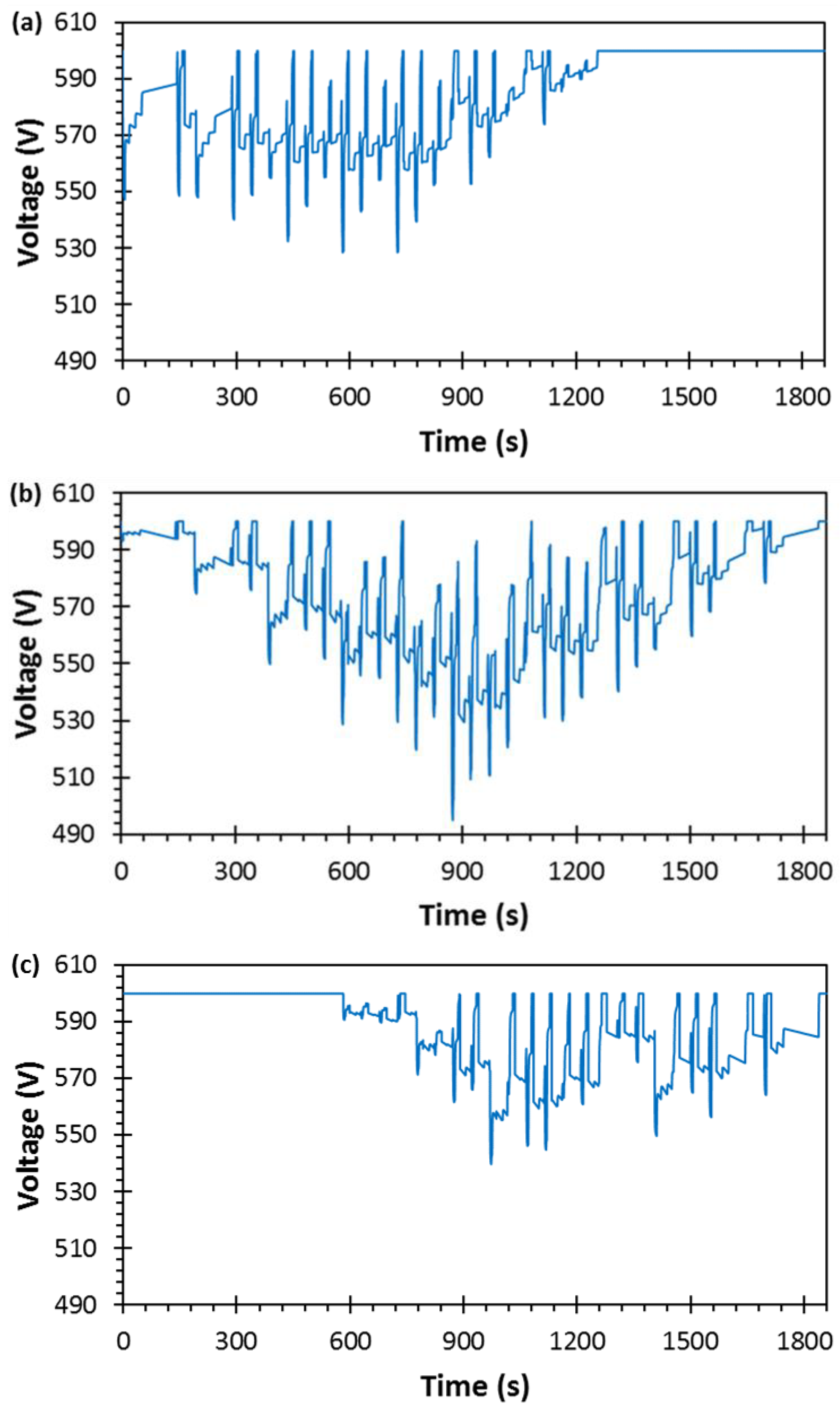
Figure 13 and Figure 14 show the voltages and power of the substations, respectively. These values are dependent on the modelled track resistance. Substation voltage and train voltages are variable due to the changes in train location and power demand. The voltages of the substations decline below the nominal voltage when the trains accelerate close to them and the voltages rise when the trains decelerate close to them. They supply power when their voltages drop below the no-load voltage and they supply no power when their voltages are equal to the no-load voltage. The substations are blocked when their voltages exceed the no-load voltage and are lower than the minimum system voltage at load, which is 400 V in this case. Under voltage is a severe issue because it can cause operational failure of the load. Moreover, it causes extra current to be supplied to meet power requirements, this increase in current results in high losses in transmission.

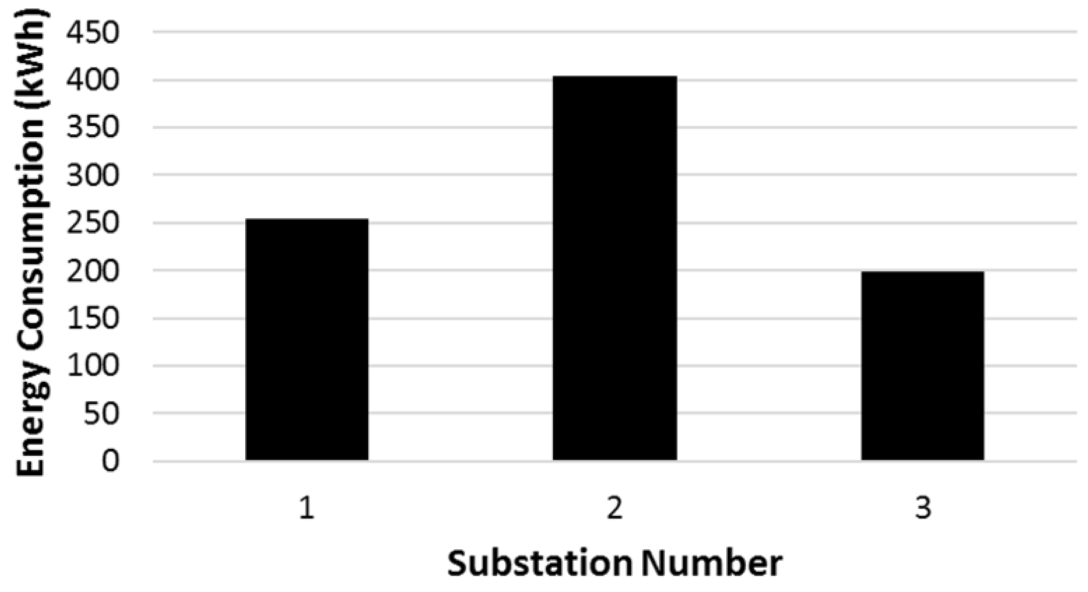
It can be noted that Substation 2, which is located in the middle of the track, is producing more power than the other two. The mean power of the substations is 0.5 MW, 0.73 MW and 0.29 MW, respectively. The energy consumption of each substation is shown in Figure 15. As a result, Substation 2 supplies more power because, in most cases, it is closer to the accelerating trains than the other two traction substations. Similarly, Substation 1 supplies more energy than Substation 3 due to its proximity to the accelerating trains at the beginning of the journey, while no trains accelerate in the vicinity of Substation 3. The highest peak power demand (3.15 MW) occurs at Substation 2.

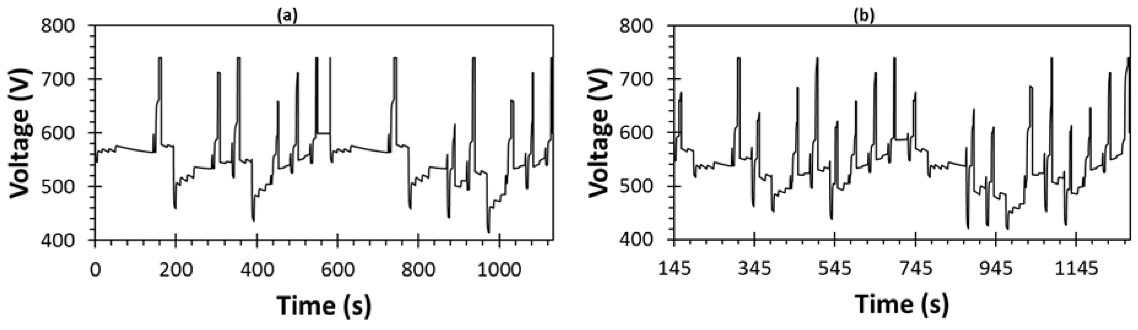
The voltages seen by all six trains are displayed in Figure 16. The rapid change in voltage is due to the change in the trains’ power demand, as well as the interactions between trains. In other words, the high transient currents that result from braking and traction cause high voltage fluctuations. When a train is in the braking mode, its voltage exceeds the substation voltage before it is controlled by the braking resistor box. If the train voltage is 400 V or below, the train motor will be shut down because the power demand cannot be met by the traction substations.

The train speeds are not assumed to be very high and their power demands change with the speed and location. The trains’ power demands change significantly from one state to another. The train is in traction mode if the train current is positive and its traction energy consumption is calculated by the integration of the train power demand as follows:

$$E_t={\displaystyle \underset{0}{\overset{T}{\int }}{I}_t\cdot V_{train}dt},$$

(6)

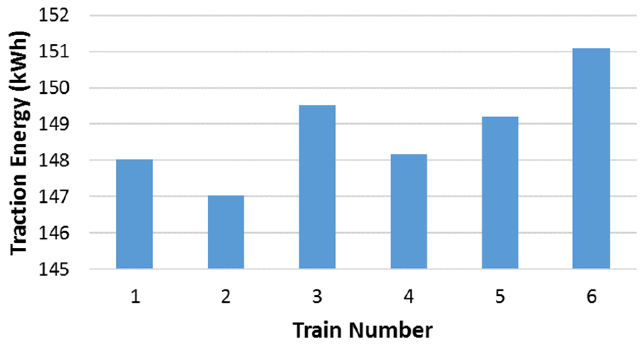
where $E_t$ is the train traction energy, $I_t$ is the traction current of the train and $V_{train}$ is the voltage seen by the train, which is the difference between the 3rd rail node and the 4th rail node. If $E_t<0$, the train is in the braking mode and $E_t>0$ implies that the train is in the motoring mode. Figure 17 shows that the highest traction energy is consumed by the last train because of the weak interaction between the running trains at the end of the entire journey.

At the beginning of the simulation, only Train 1 is running, which causes the voltage at the train’s location to increase significantly when the train is braking and the voltage declines rapidly when the train is accelerating. However, when other trains are running on the track, the voltage seen by each train does not depend solely just on that train’s behaviour but also on the other trains on the track. It is evident that the voltages at a train’s location reach very high values when a train brakes between any two consecutive substations. Similarly, the highest voltage drop seen by the trains occurs when the trains accelerate between two substations. It is observed that the shorter the distance between the trains, the higher the interactions between them will be.

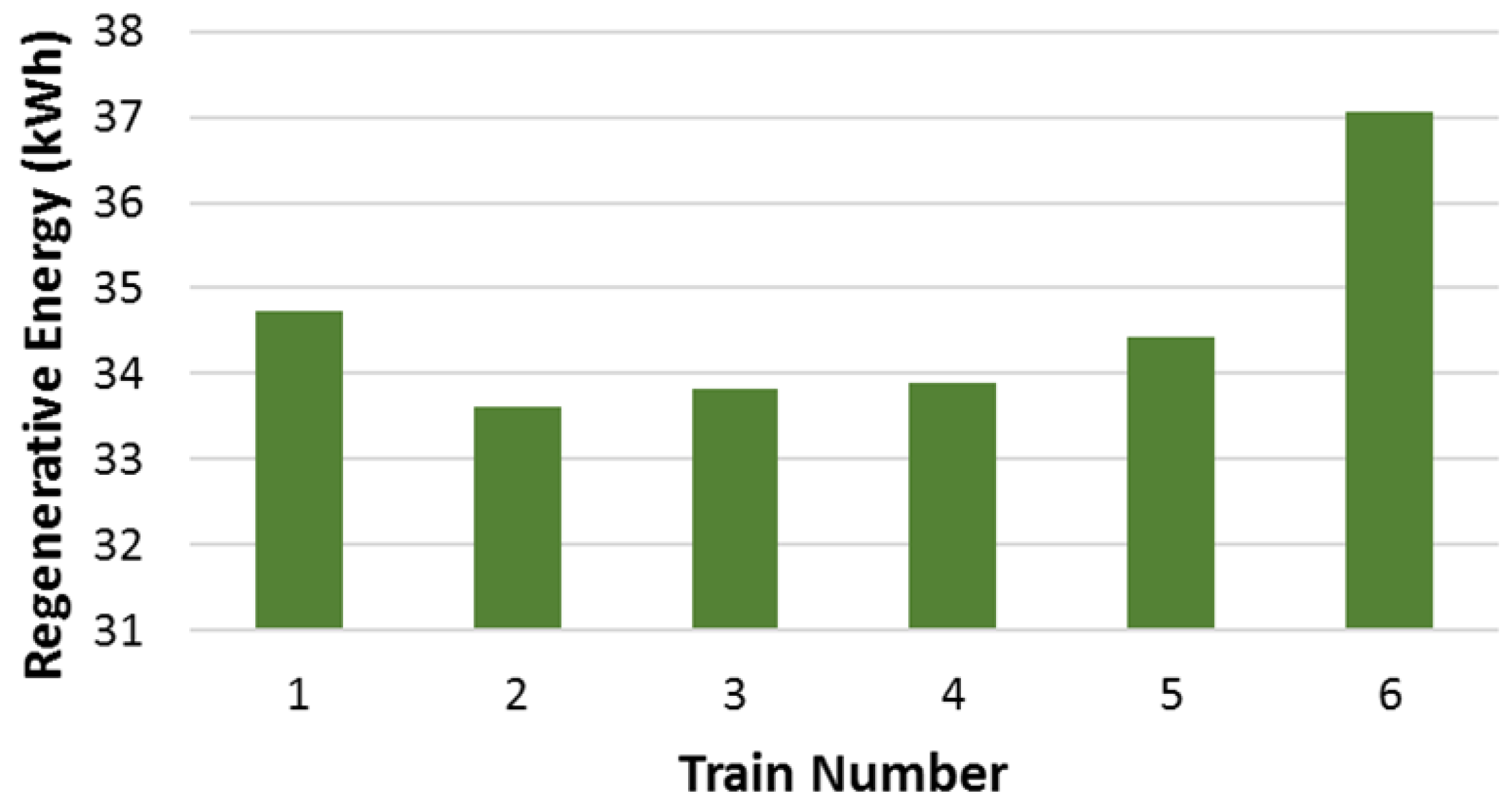
Power exchange between trains occurs only if there are multiple trains running on the track. The regenerative braking power is consumed by other trains that are running simultaneously on the same section. In the case of just one running train, the total regenerative power is dissipated in the braking resistor. Combined, the trains regenerate 24.2% of the total traction energy for one cycle. In Figure 18, it can be seen that the first and the last train regenerate more energy than do others due to a very low traffic density. In low traffic, the voltage drop on the track will be lower than that in high traffic. Therefore, trains regenerate more energy in low traffic because the regenerative energy depends strongly on trains voltages as can be seen in the following equation:

$$E_r={\displaystyle \underset{0}{\overset{T}{\int }}{I}_r\cdot V_{train}dt},$$

(7)

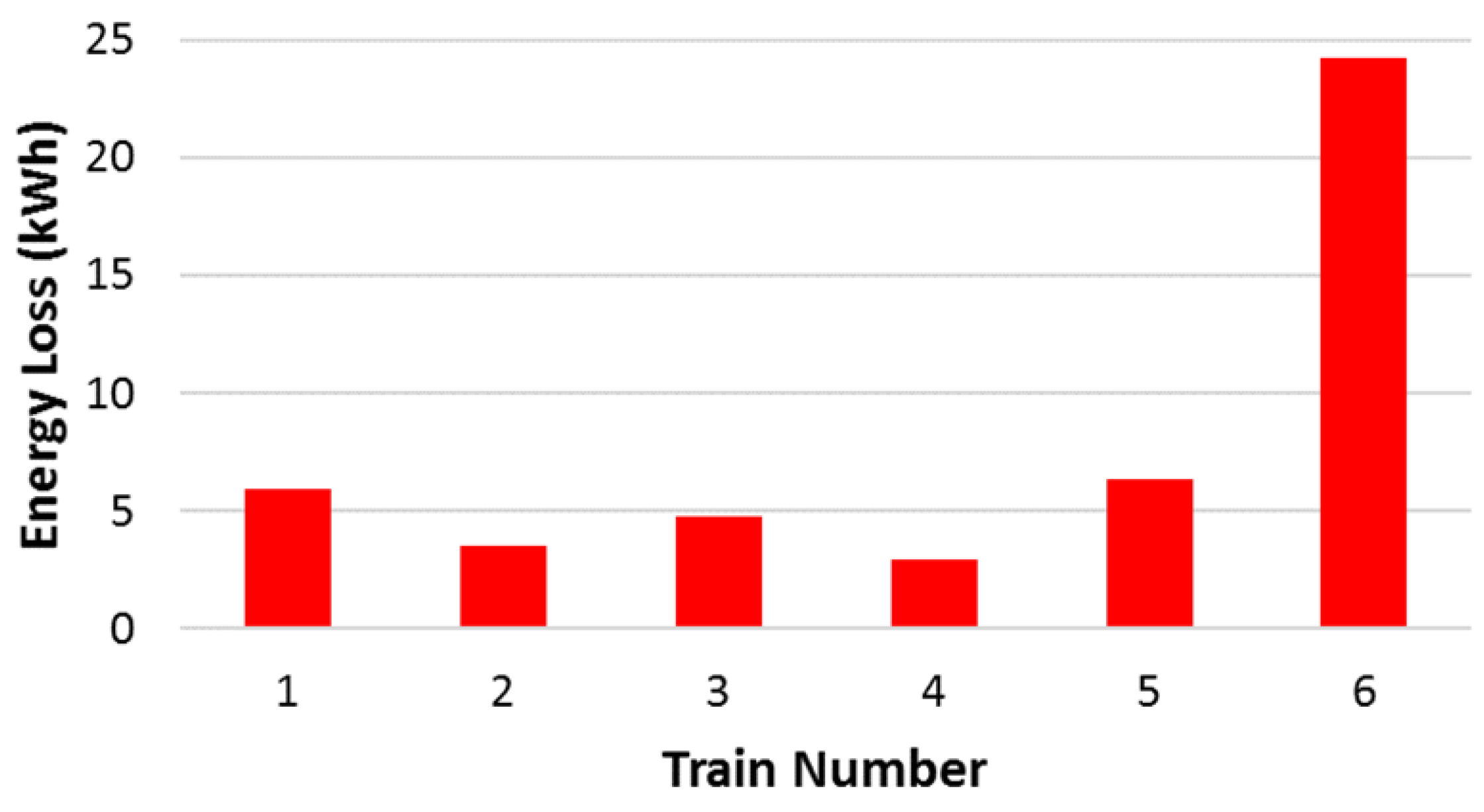
where $E_r$ is the train braking energy and $I_r$ is the braking current of the train. The unexploited braking energy is dissipated in the braking resistors. The unused braking energy of each train is shown in Figure 19 and is calculated by:

$$E_{cb}={\displaystyle \underset{0}{\overset{T}{\int }}{I}_{cb}\cdot V_{train}dt},$$

(8)

where $I_{cb}$ is the current passing through the braking resistor of the train.

5. Consideration for Braking Energy

The shorter the distance between the trains, the greater the exchange of power between them will be. Effective power exchange between running trains can reduce the power consumption of the rectifier substations, which reduces the electricity costs. Therefore, utilisation of the regenerative energy should be considered for the study into ESSs. Different energy exploitation scenarios are considered here. The utilisation factor ${\eta }_{utilisation}$ measures the percentage of the used braking energy relative to the total braking energy as follows:

$${\eta }_{utilisation}=\frac{{\displaystyle \sum E_r-{\displaystyle \sum E_{cb}}}}{{\displaystyle \sum E_r}}\times 100\%,$$

(9)

where ${\displaystyle \sum E_r}$ is the total regenerative energy by the braking trains and ${\displaystyle \sum E_{cb}}$ is the total dissipated braking energy in the braking resistors of the trains.

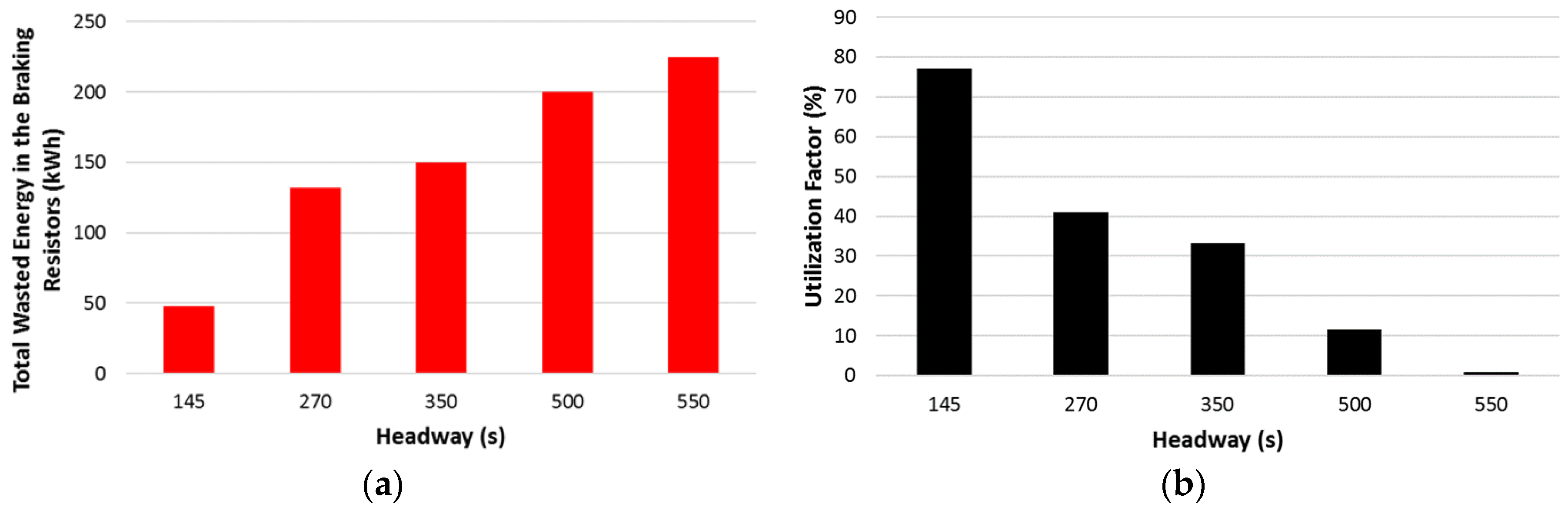
In the first scenario, six trains are running on a 9 km railway with a 145 s interval between consecutive trains. The utilisation factor for the first case study was 77%, meaning that minimal energy was wasted during braking, due to high train circulation. It is calculated that the kinetic energy loss is approximately 16% of the total energy supplied by the substations. The second scenario is similar to the first one but the headway is increased to 270 s and the utilisation factor is thus reduced to 41%. Unsurprisingly, when the headway is increased to 550 s, the power utilisation becomes very poor. It is calculated that the utilisation factor was 1%, due to the lack of accelerating trains to consume the regenerative power.

Figure 20a shows the total wasted energy during braking for the same system but with different departure intervals for one complete cycle. To reduce the voltage drop in the line, short electrical sections are considered. As a result, there is always lack of trains in power demand that can consume the available regenerative power. It can be seen that increasing the headway increases the losses in the braking resistors because traffic density is low. Therefore, the probability of power exchange between simultaneously braking and accelerating trains is higher for short headways than for long headways due to having several trains on the track.

The receptivity of the railway line, which is the capability of the trains to accept the available regenerative energy by decelerating trains, reduces with increasing headway, as shown in Figure 20b. However, that is not always the case as, for example, if all trains start accelerating and decelerating simultaneously, then the dumped energy in the onboard braking resistors will be very high and the utilisation factor will be deficient although the headway is short. In other words, the simultaneous presence of braking and accelerating trains is the main factor in improving the line receptivity. In decupled railways, receptivity of lines deteriorates with the increase of headway due to the high likelihood of consecutive trains being separated by different electrical sections. The headway parameter is crucial to optimise energy efficiency in multi-train railways.

It can thus be concluded that the lower the number of trains running simultaneously on the track, the lower power utilisation in the railway will be, as discussed in References [25,26]. Similarly, increasing the headway in multi-train systems decreases the power utilisation in the railway. It is proposed that storing the regenerative energy in ESSs, instead of dissipating it in the rheostats, will enable the receptivity of the railway to be controlled offering increased energy efficiency and relaxing headway restrictions.

Although headway significantly affects the energy efficiency, it is not always feasible to change the headway to save energy. In other words, long headways reduce the number of passengers onboard and very short headways might cause safety issues due to the small distances between trains. To sum up, electric railway receptivity can be affected negatively by a considerable distance between braking and accelerating trains, as the available regenerative power on the line exceeds the power demand and the no-load voltage. In some electric railways, the no-load voltage is high to reduce voltage dips and line losses. However, this results in reducing the line receptivity by limiting the voltage range of the decelerating trains to supply their regenerative power. This issue could be overcome by changing transformer taps to modify the no-load voltage according to the line receptivity.

6. Model Validation

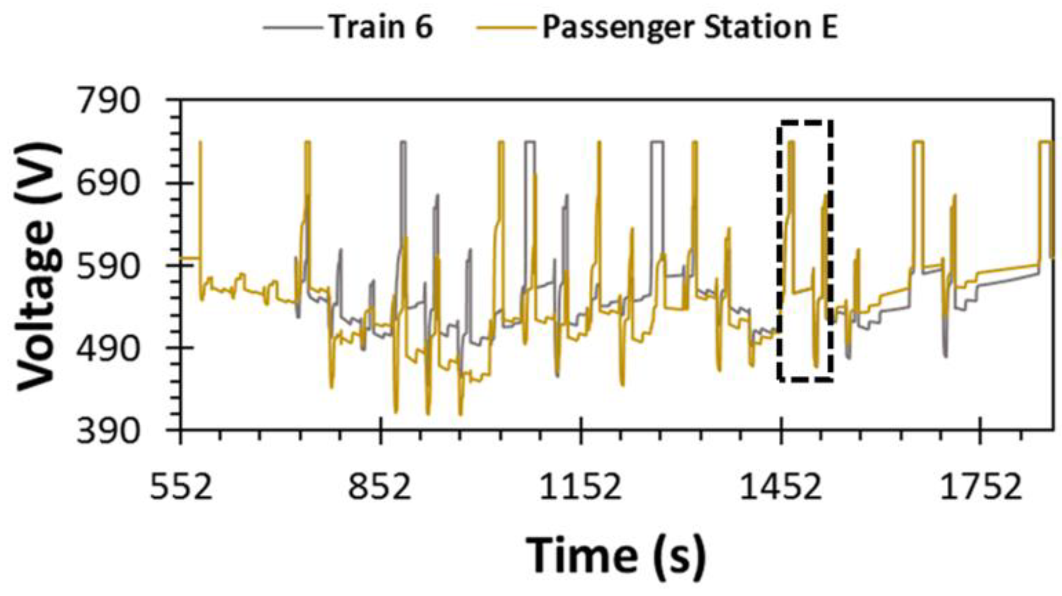
The validation of the model presented in this paper is discussed here using a number of methods. The passenger stations are stationary and are situated at different locations along the track. The trains are in motion and they all pass these stations at a known time. Measuring the passenger stations’ voltages and the voltages seen by the trains, these should be matched at that time when a train is located at a certain station. From the data reported in Figure 3, it can be deduced that Train 1 reaches Interstation F at 940 s and dwells for 30 s and during this time, voltage matching occurs, as shown in Figure 21. Another case is considered in Figure 22 and it shows a match between the passenger station’s voltage and the train’s voltage when the train and the station are at the same location on the track. Noticeably, high voltage calculation accuracy is proved notwithstanding the dynamic behaviour of the electric railway.

The model was also validated by summing the total power generation minus the total power demand, which must equal to zero. In other words, the substations’ output energy and the trains’ regenerative energy should be equal to the trains’ energy consumption and the total losses in the system, as follows:

$${\displaystyle \sum E_s+{\displaystyle \sum E_r={\displaystyle \sum E_t+{\displaystyle \sum E_{linelosses}+{\displaystyle \sum E_{substationlosses}+{\displaystyle \sum E_{cb}}}}}}},$$

(10)

where ${\displaystyle \sum E_s}$ is the total energy consumption of all substations, which is the time integral of the power shown in Figure 14; ${\displaystyle \sum E_{linelosses}}$ denotes the total energy losses in the 3rd and 4th rail; and ${\displaystyle \sum E_{substationlosses}}$ represents the total energy losses in the internal resistors of the substations, which represents the losses in the substation transformers and rectifiers. The losses in the system is shown in

Table 2. Energy Consumption and Losses in the System.

${\displaystyle \sum {\mathit{E}}_{\mathit{s}}}(\mathbf{kWh})$	${\displaystyle \sum {\mathit{E}}_{\mathit{r}}}(\mathbf{kWh})$	${\displaystyle \sum {\mathit{E}}_{\mathit{t}}}(\mathbf{kWh})$	${\displaystyle \sum {\mathit{E}}_{\mathit{l}\mathit{i}\mathit{n}\mathit{e}\mathit{l}\mathit{o}\mathit{s}\mathit{s}\mathit{e}\mathit{s}}}(\mathbf{kWh})$	${\displaystyle \sum {\mathit{E}}_{\mathit{s}\mathit{u}\mathit{b}\mathit{s}\mathit{t}\mathit{a}\mathit{t}\mathit{i}\mathit{o}\mathit{n}\mathit{l}\mathit{o}\mathit{s}\mathit{s}\mathit{e}\mathit{s}}}(\mathbf{kWh})$	${\displaystyle \sum {\mathit{E}}_{\mathit{c}\mathit{b}}}(\mathbf{kWh})$
857.94	207.5	893.06	82.44	50.76	47.69

.

From the above results, it can be established that the two sides of Equation (10) are equal with an error of 0.79%, which is acceptable due to the transients created by the switches in the simulation model.

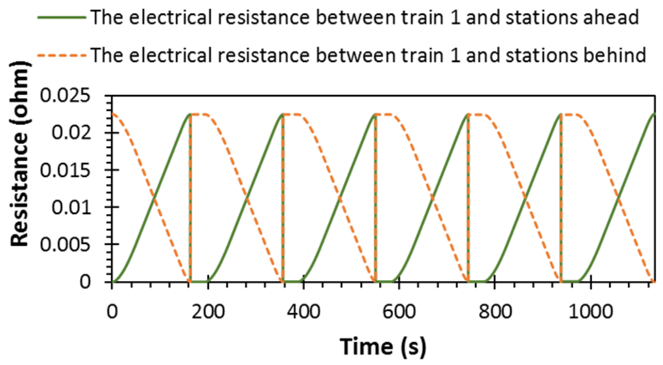
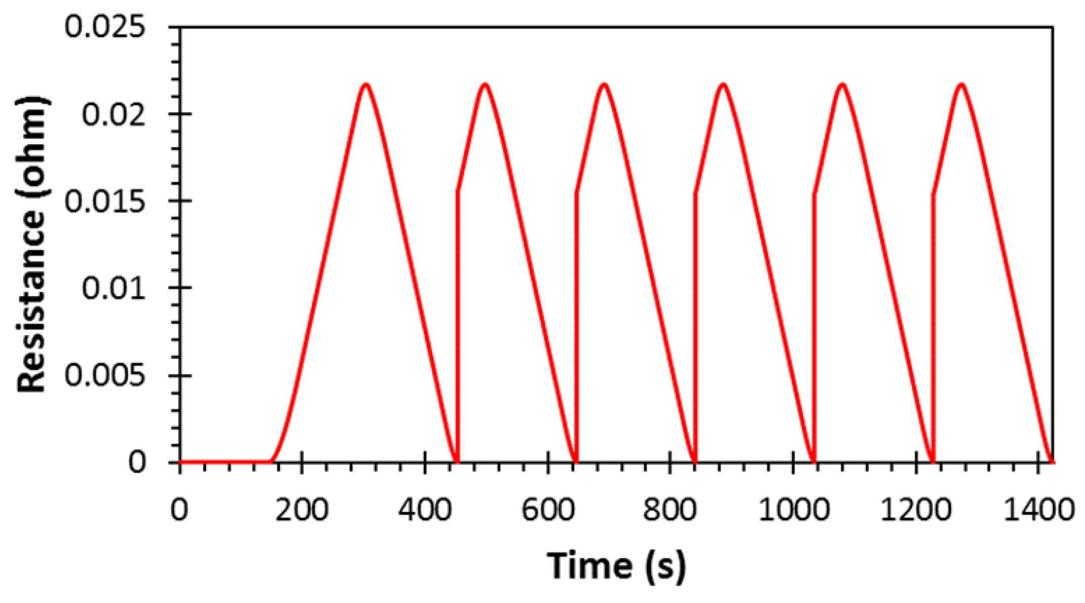
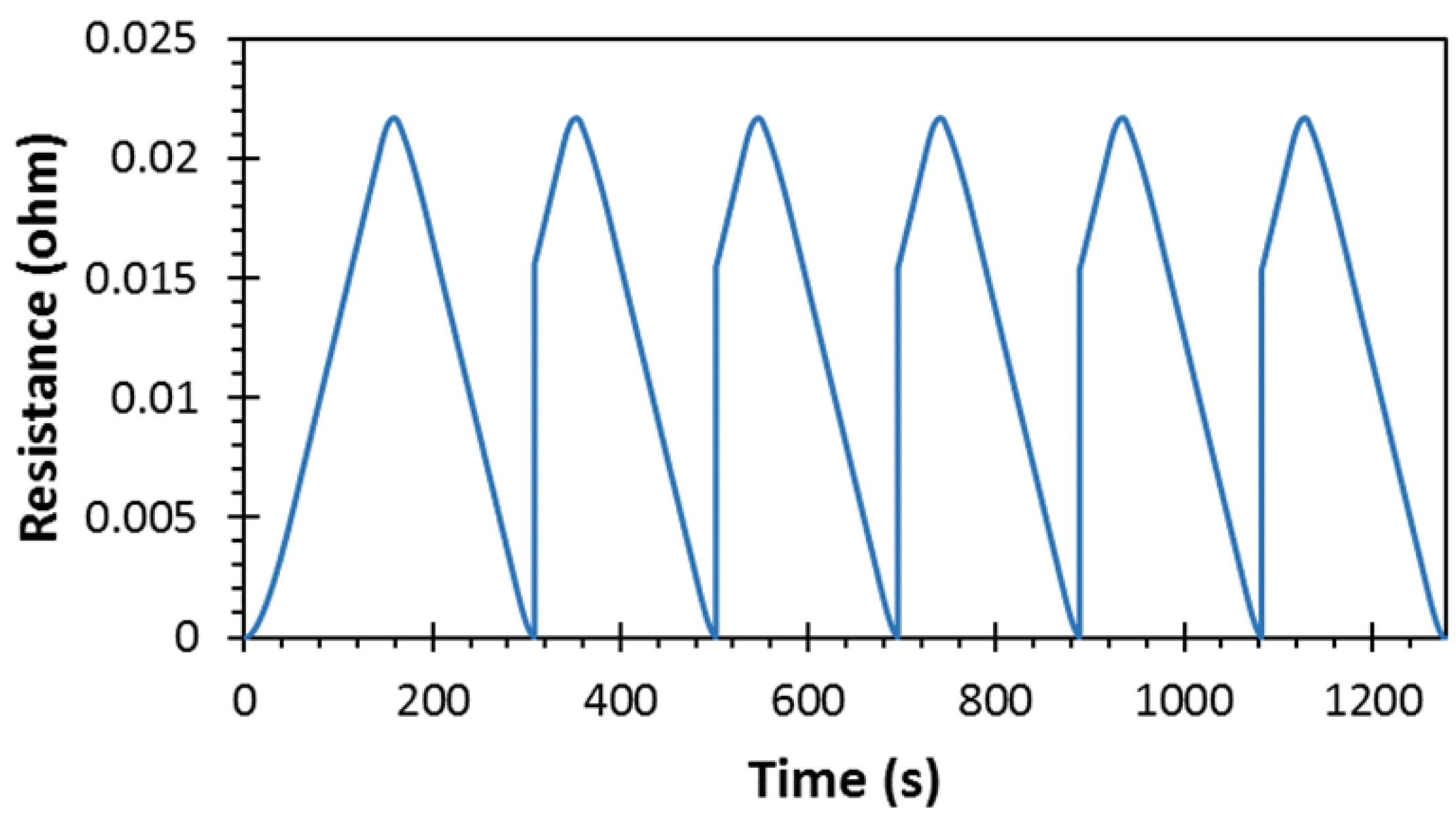
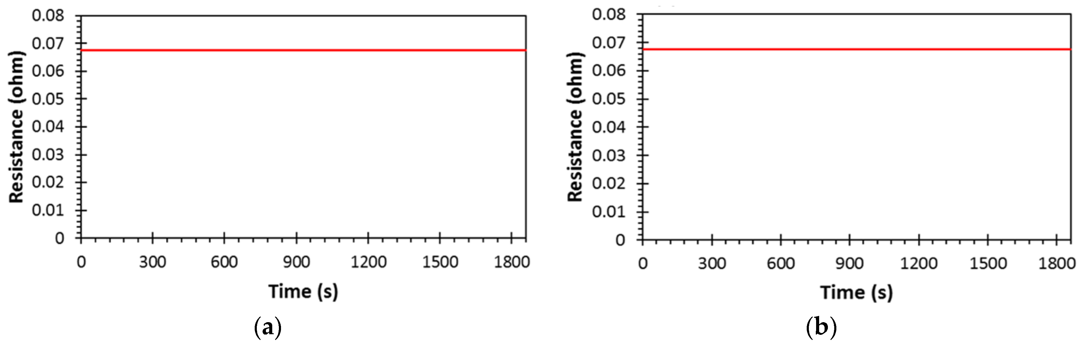
Finally, the track total length of 9 km is divided electrically into two sections by placing three substations. Each section’s electrical resistance is calculated by the multiplication of the section length and the electrical rail resistance per km. The transmission line between each two consecutive substations is divided into resistors with different values, which depend on the trains’ locations. However, the total electrical resistance of the first section of the rail track should always be equal to 67.5 mΩ, which is the same for section two. In other words, the equations used to calculate the electrical resistance difference between the trains, as well as between the trains and the virtual stations, are merely splitting the total track’s electrical resistance based on the trains’ locations but it should not change the total section resistance. Therefore, the sum of those resistances should always be 67.5 mΩ, irrespective of the trains’ locations. Figure 23 shows perfect matching between the total electrical resistance and the sum of the electrical resistances of the changing network configuration by applying (4) and (5).

7. Conclusions

The purpose of this work was to develop an electrical model that describes the effect of a moving train on an electric DC railway. The trains and rail track characteristics were assumed to be variable and needed to be updated at each time step. The mechanical model was coupled with the electrical model to investigate the impact of trains on the electrical power system. The trains’ measured data were considered to be inputs into an existing electric railway system. The electrical system was responsible for solving the power flow instantly with the inputs from the mechanical model.

Moreover, in this paper, a simplified test scenario was presented, comprising of six trains running on a 9 km rail track, in order to validate the model against the expected observations. The model proposed here can provide the track and train voltages at any location, along with power flows. Hence, this model can be used to study the effects of energy storage on the railway system and to optimise it for solutions. Consequently, it will be possible to design onboard or stationary ESSs to import and export energy with accurate energy calculations by voltage control. The proposed simulation method is simple, accurate and adaptable to changes in the circuit configuration. The simulation model was validated via different methods. As a consequence of this approach, iterative methods for solving the nonlinear equations characterising the system have been avoided.

The feeding network voltage reaches high values during braking. To protect the network from overvoltage, braking resistors are connected in parallel with the trains to burn the excess energy. The dissipated energy in the braking resistors represents 26.4% of the total losses in the single electric railway. The issue of voltage drop in the track line was not discussed in this paper and needs to be considered in the future. Therefore, it is recommended to use ESS to store the excess energy instead of burning it in the braking resistor box. Thereafter, the energy stored in the ESS can be used to protect the network from undervoltage and overvoltage. As a result, expensive substation upgrades to improve energy efficiency of existing electric railways will be avoided.