A Passenger-Oriented Optimization Model for Implementing Energy-Saving Strategies in Railway Contexts


Department of Civil, Architectural and Environmental Engineering, Federico II University of Naples, Via Claudio 21, 80125 Naples, Italy
*
Author to whom correspondence should be addressed.
Energies 2018, 11(11), 2946; https://doi.org/10.3390/en11112946
Submission received: 5 October 2018
/
Revised: 17 October 2018
/
Accepted: 22 October 2018
/
Published: 29 October 2018
(This article belongs to the Special Issue Selected Papers from EEEIC 2018—18th International Conference on Environment and Electrical Engineering)
Abstract
:Rail and metro systems are characterized by high-performing and environmentally friendly features that make them a crucial factor for driving modal split towards public transport modes, thus reducing private car use and related externalities (such as air and noise pollution, traffic congestion and accidents). Within this framework, the implementation of suitable energy-saving policies, allowing to reduce energy consumption, but, at the same time, preserving timetable stability and passengers’ satisfaction, may turn out to be imperative. In particular, this study aims to develop an analytical framework for properly supporting the implementation of eco-driving strategies in a passenger-oriented perspective. An application to a rail line in southern Italy is performed so as to demonstrate the usefulness of the proposed approach in determining the optimal compromise between energy reductions and travel time increases.
1. Introduction
Rail and metro systems, thanks to their high performance and sustainability characteristics, have a key role with a view to reducing side effects related to transport sector, thus properly promoting a sustainable development of urban and metropolitan regions [1]. In particular, transport modes based on railway technology present a more favorable ratio between operational costs (including energy consumption) and transport capacity with respect to other mobility systems. Therefore, the necessity of fully exploiting such energy efficiency and the ever-increasing cost of energy resources make the implementation of energy-saving measures a crucial factor in the management of rail systems.
Within this framework, our aim is to provide a decision support system (DSS) for the implementation of eco-driving strategies in the case of rail/metro systems. More in detail, such strategies can follow different approaches; however, whatever the implemented method, they produce an increase in train running times which provides two main implications. First of all, the adoption of such measures is feasible only if there is an extra-time availability to be exploited for compensating the increase in running times, without prejudicing timetable stability. These time resources have to be adequately designed in the timetable planning phase and, therefore, a proper tool for allowing a reliable estimation of them has been developed. The second implication concerns service quality and passengers’ satisfaction. Indeed, an increase in train running time is equivalent to an increase in user travel times, with a consequent degradation in system performance. Hence, the aim is to provide a suitable tool for evaluating the trade-off between the reduction in energy consumption and the increase in passenger discomfort. For this twofold purpose, proper simulation models and travel demand estimation techniques have been applied. Moreover, the interaction between rail service and passenger flows has been modelled by means of a microscopic approach. Finally, a bilevel constrained optimization problem has been formulated and solved in the case of a real rail network, so as to show the effectiveness of the proposed methodology.
Specifically, in this paper, we provide an extension of the authors’ research in determining the optimal compromise between energy reductions and travel time increases [2], proposed at the 18th IEEE International Conference on Environment and Electrical Engineering (IEEE EEEIC 2018) and 2nd Industrial and Commercial Power Systems Europe (I&CPS 2018). More in detail, the work was enriched by deeply analyzing the analytical formulation of the problem and investigating related theoretical properties. Moreover, a bilevel solution algorithm was developed and numerical applications were extended.
The paper is organized as follows: Section 2 analyzes the main contributions in the literature; Section 3 provides the analytical formulation of the proposed approach with the definition of related theoretical properties and adopted solution algorithms; Section 4 applies the proposed methodology in the case of a regional rail line; finally, conclusions and research prospects are summarized in Section 5.
2. Literature Review
Researchers and practitioners have developed different strategies, such as the adoption of eco-driving profiles, the regenerative braking, the adjustment of timetables, the exploitation of on-board and way-side storage systems, the use of reversible substations. Clearly, they are strictly related to each other. In particular, the design of energy-efficient speed profiles consists in identifying the pattern which minimizes the tractive energy consumption, given a running time to be respected (see, for instance, [3,4,5]); while, strategies based on the exploitation of regenerative braking aim to reuse the amount of kinetic energy produced during the braking phase by converting it back to the electrical one. In this case, the traction motor acts also as a generator and the recovered energy can be used at the exact time or stored for later use by means of energy storage devices. For instance, an on-board storage device allows to temporarily accumulate the excess regenerated energy and release it for the next acceleration phase of the same train (see, for instance, [6,7,8]); while, the aim of a wayside storage device is to release it when required for other convoys’ acceleration (see, for instance, [9,10]). On the other hand, when no storage devices are available, a timetable optimization, aimed at synchronizing acceleration and deceleration phases of convoys operating in the network, represents a key task for maximizing the receptivity of the line (see, for instance, [11,12,13,14]). Additionally, the role of an energy-efficient timetabling phase lies in a suitable design of all operational times involved, such as running times, buffer times, dwell times and reserve times [15,16,17,18]. Moreover, by means of reversible or active substations, the regenerated energy can also be traced back to the medium voltage distribution network [19,20]. An extensive overview of regenerative braking issues and energy storage systems, together with the above-mentioned related concerns, can be found, respectively, in [21,22].
This work, instead, is focused on strategies involving the design of suitable speed profiles and the optimization of operational parameters within the timetable by taking into account effects on user perspectives. Indeed, recently, numerous studies have been developed for analyzing user behaviors and related quality perceptions (see, for instance, [23,24,25,26,27,28,29,30,31,32,33,34,35]) in the case of transportation systems, including rail and metro systems.
Specifically, according to the literature, the above-mentioned techniques can be applied separately, by addressing individually the design of energy-efficient driving profiles [36,37] and the optimization of operational times within the timetable [38,39] or, more frequently, in an integrated framework. In this context, Li and Lo [40] proposed a train control approach, based on an optimization model, which combines energy-efficient timetables and speed profiles within a dynamic framework providing the adjustment of the cycle time according to travel demand changes. Moreover, Scheepmaker and Goverde [41] developed a nested optimization framework in which the optimal cruising speed is defined by means of the outer loop of the Fibonacci algorithm [42,43]; while, in the inner loop, the bisection method computes, for the given cruising speed, the optimal switching points of the coasting phase. Furthermore, Sicre et al. [44] proposed a simulation-based optimization procedure in which the simulation model provides the most energy-efficient driving profile, by computing energy consumption Pareto curves for each stretch, and the optimization tool allocates the total running reserve time available in the most efficient way among the different stretches. Finally, Feng et al. [45] enriched the common optimization framework, which combined energy control strategies with a suitable design of operational times, by performing the estimation of dwell times at stations as flow-dependent factors. It is worth noting that both manual [46,47,48] and automatic [49,50,51] driving systems have been considered.
As regard to the adopted methodological approaches, the most common methods for analyzing these strategies are based on integrated simulation-optimization techniques, both in off-line [52,53] and real-time [54,55,56,57,58,59,60,61] contexts. On the other hand, analytical approaches for modelling the implementation of ES strategies can be found in [4,62,63,64].
Several works merged the energy-saving perspective with operational issues. Within this framework, several authors [65,66,67] analyzed the relation between energy-efficient strategies and stability of the planned timetable; Feng et al. [68] evaluated the utilization rate of train capacity resulting from the implementation of energy-saving strategies; Canca [69] compared the minimum-energy timetable with those obtained by taking into account also rolling stock and other operational costs. Authors’ proposal, instead, consists in a passenger-oriented bi-objective framework, in which the energy perspective is combined with the evaluation of passengers’ satisfaction, expressed in term of user generalized cost. The aim is to identify the optimal compromise between energy reductions and travel time increases, thus allowing a minimization of consumption without penalizing passengers’ needs.
3. The Proposed Methodology
As shown by [70,71], in the case of a rail (or metro) line with two-track sections, the minimum time required by a rail convoy to perform a complete trip may be calculated as follows:
with:
where is the minimum cycle time; and are the Total Running Times associated, respectively, with the outward trip (ot) and the return trip (rt) in the Time Optimal (TO) condition; and are the Total Dwell Times associated, respectively, with the outward trip (ot) and the return trip (rt); and are the inversion times (i.e., times spent to prepare the rail convoy to perform the subsequent trip) associated, respectively, with the outward trip (ot) and the return trip (rt); and are the running times associated, respectively, with links belonging to the outward trip (lot) and the return trip (lrt) in the Time Optimal (TO) condition; and are the dwell times associated, respectively, with station platforms in the case of outward trip (sot) and return trip (srt).
Since terms of Equation (1), as well as terms of Equations (2)–(5), have to be considered as realizations of random (i.e., stochastic) processes due to their variability, the minimum cycle time may be formulated as follows:
with:
where is the mathematical expectation (i.e., the first moment or mean) of variable ; is the random residual of ; is the statistical distribution of ; is the vector of parameters of statistical distribution .
Since a delay occurs when the real cycle time is higher than the planned one (i.e., a train arrives later than scheduled), in order to minimize delays and, hence, assure timetable stability, it is necessary to adopt proper buffer times for compensating time increases, that it:
where is the planned cycle time; is the Total Buffer Time.
Increases in cycle time with respect to the average value may be compensated until the buffer time is reached. This implies that a train may respect the timetable whenever the increase is not higher that buffer time value, that is:
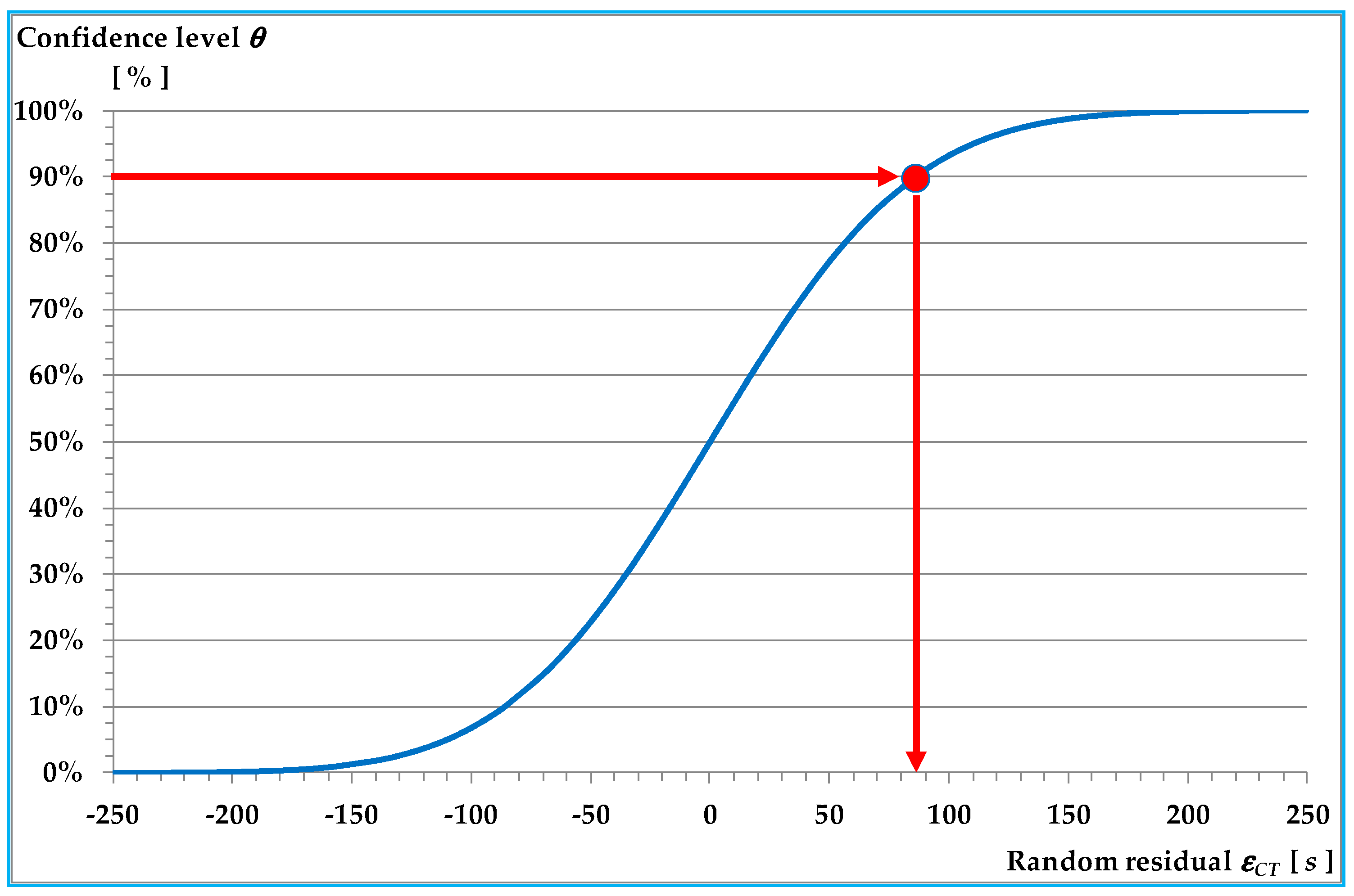
Since the statistical distribution of is known (or may be determined), it is possible to calculate the value of buffer time for any fixed confidence level by means of Equation (7). Indeed, a planned cycle time respects the timetable with a confidence level equal to only if:
which, by means of Equations (6) and (8), may be expressed as:
The cumulative distribution of expresses the delay (when is non-negative) or the advance (when is negative) of a train with respect to its average trip duration (i.e., value). Hence, as shown in Figure 1, once fixed a confidence level , it is possible to determine the corresponding value of random residual , which expresses the maximum delay associated with confidence level . Then, if we assume a buffer time equal to this maximum delay, the planned cycle time will be not lower than the real cycle time with a confidence level . Obviously, higher the confidence level, higher the value of buffer time .
Conventionally, in order to preserve departure times at the terminals, the buffer time is calculated separately for the outward trip and the return trip, that is:
where and are the buffer times associated, respectively, with the outward trip (ot) and the return trip (rt).
The number of rail convoys required to perform a frequency service on a single line may be calculated as follows:
where is the number of rail convoys; is the service cycle time; is the average headway between two successive rail convoys.
Since the number of rail convoys to adopt to perform the service has to be a positive integer number (i.e., NC ∈ Z+), Equation (9) may be expressed in terms of planned cycle time as follows:
Hence, it is possible to express the service cycle time as follows:
with:
where is the Total Layover Time in the Time Optimal (TO) scenario which expresses the time that a train spent at the initial station waiting for the departure time according to the planned timetable. However, the layover time is defined separately for the outward trip and the return trip for preserving departure times at the terminals, that is:
where and are the layover times associated, respectively, with the outward trip (ot) and the return trip (rt), in the case of the Time Optimal (TO) scenario.
Let be the partition rate of the , we may express the layover times as follows:
with .
Since buffer and layover times express phases where the train is steady on the track, in order to preserve the headway, it is necessary to satisfy the following constraints:
which imply constraints on the partition rate of the and the number of rail convoys. Specifically, these constraints may be expressed as follows:
Moreover, since the layover time allocation (i.e., parameter ) affects the minimum headway of the line, it is necessary to verify whether the proposed service is feasible by means of the following condition:
where is the minimum headway of the line, depending on parameter .
The implementation of Energy Saving Strategies (ESSs) consists in adopting suitable strategies (such as proper speed profiles and/or the use of recovery devices) so to reduce energy consumption, that is:
where and are the Total Energy Consumptions associated, respectively, with the implementation of the Energy Saving Strategy (ESS) and the Time Optimal (TO) scenario without any recovery device.
Neglecting the use of recovery devices, these strategies imply an increase in running times, that is:
with:
where and are the Total Running Times associated, respectively, with the outward trip (ot) and the return trip (rt) in the case of Energy Saving Strategy (ESS) implementation; and are the running times associated, respectively, with links belonging to the outward trip (lot) and the return trip (lrt) in the case of Energy Saving Strategy (ESS) implementation. Hence, to preserve service performance in terms of timetable stability and service frequencies, it is necessary to compensate for the increase in running times by means of reduction in layover times, that is:
which imply:
where and are the layover times associated, respectively, with the outward trip (ot) and the return trip (rt), in the case of the Energy Saving Strategy (ESS); is the Total Layover Time in the case of Energy Saving Strategy (ESS).
3.1. Optimization Problem Formulation
In order to reduce the negative impacts on passengers due to the implementation of Energy Saving Strategies, it is necessary to identify the optimal compromise between travel time increase and energy reduction. Hence, assuming the adoption of a strategy based on the definition of lower speed limits (for details, see [70,71]), we propose to solve the following bilevel optimization problem, where the upper level, whose aim is to identify the partition rate, which minimizes an objective function, may be formulated as follows:
subject to:
with:
and the lower level, whose aim is to identify speed limits which maximize running times, may be formulated as follows:
subject to:
where is the optimal value of ; and are the optimal value of and ; and are the speed limits associated, respectively, with the outward trip (ot) and the return trip (rt); is the objective function to be minimized in the upper level; is the Total Energy Consumption in the case of Energy Saving Strategy (ESS); is the Total User Generalized Cost in the case of Energy Saving Strategy (ESS); is a parameter which expresses the monetary cost of the energy (i.e., Value Of Energy); is the daily number of complete trips depending on headway and number of rail convoys ; and are the Energy Consumption associated, respectively, with the outward trip (ot) and the return trip (rt) in the case of Energy Saving Strategy (ESS); and are the portion of associated, respectively, with the outward trip (ot) and the return trip (rt), i.e., + = ; is the tractive effort at rail wheels which depends on travel speed; and are the instantaneous travel speeds associated, respectively, with the outward trip (ot) and the return trip (rt) in the case of Energy Saving Strategy (ESS) and depending on speed limits and , and the generic time instant ; is the generic time instant; in the generic infinitesimal time interval; is a parameter which expresses the monetary value of the time spent on-board by passengers (i.e., Value of the On-Board Time); and are the on-board times associated, respectively, with links belonging to the outward trip (lot) and return trip (lrt) in the case of Energy Saving Strategy (ESS), depending on speed limits and ; and are the flows of passengers on board the rail convoy associated, respectively, with links belonging to the outward trip (lot) and return trip (lrt) during the i-th trip; is a parameter which expresses the monetary value of the time spent by passengers on the platform waiting for a train (i.e., Value of the Waiting Time); and are the waiting times associated, respectively, with station platforms in the case of outward trip (sot) and return trip (srt), depending on headway ; and are the flows of passengers waiting for a train associated, respectively, with station platforms in the case of outward trip (sot) and return trip (srt) during the i-th trip; and the value assumed by speed functions (i.e., driving speed profiles) associated, respectively, with the outward trip (ot) and the return trip (rt) in the case of Energy Saving Strategy (ESS) at generic time interval .
The upper level (i.e., Equation (15)) consists in determining the optimal value of which minimizes the objective function , having fixed the headway (), the number of rail convoys () and having determined the corresponding speed limits ( and ) by means of the lower level problem (i.e., Equations (24) and (25)).
The objective function , as shown in Equation (19), is equal to the sum of monetary values of consumed energy () and times spent by passengers during their trips (). In particular, the consumed energy may be calculated by integrating the power function (i.e., the product between the tractive effort and the instantaneous speeds and ) by means of Equations (20)–(22). Likewise, the user generalized cost may be calculated as the sum of on-board times ( and ) and waiting times ( and ) spent by each passenger, appropriately multiplied by the corresponding perception weight (i.e., and ).
Constraints (16)–(18) reiterate the considerations highlighted by Equations (12)–(14) concerning feasibility sets of parameters.
The lower level (i.e., Equations (24) and (25)) consists in determining, for any fixed value, the maximum values of speed limits ( and ) which maximize the use of layover times ( and ). Indeed, constraints (26) and (27) impose driving speed profiles ( and ) which respect the speed limits ( and ). Likewise, constraints (28) and (29) allow an increase of the Total Running Times in the case of Energy Saving Strategy ( and ), with respect to the corresponding values in the case of Time Optimal scenario ( and ), at most equal to the layover times ( and ).
3.2. Theoretical Properties of the Optimization Problem
In order to verify the feasibility of the proposed optimization problem, it is necessary to state the existence and the uniqueness of the optimal solution by investigating theoretical properties of the upper and lower level problems.
Theorem 1.
The upper level has at least one solution if equations described in Section 3 are satisfied.
Proof.
Optimization problem (15) has at least one solution if:
- Objective function is defined in a non-empty and compact (i.e., closed and limited) set;
- Objective function is continuous in its definition set, that is:where is the definition set of .
In the case of problem (15), once fixed the headway (), the number of rail convoys () and having determined the corresponding speed limits ( and ) by means of the lower level problem (i.e., Equations (24) and (25)), objective function depends only on parameter whose definition set is expressed by constraint (16). Hence, the definition set satisfies the non-emptiness and compactness conditions. Moreover, since function may be expressed as a compound function of continuous functions, the objective function is continuous.
Since both conditions on objective function are satisfied, the upper level has at least one solution (existence property). □
Theorem 2.
The upper level has at most one solution if equations described in Section 3 are satisfied.
Proof.
Optimization problem (15) has at most one solution if objective function is convex and defined on a convex set.
As shown in the proof of Theorem 1, function is defined on a non-empty and compact set and, therefore, it is defined on a convex set.
In order to show the convexity of function , it is necessary to consider that a variation in affects:
- according to a non-decreasing function (since an increase in provides an increase in corresponding layover time which may imply an increase in running times);
- according to a non-increasing function (since an increase in provides a decrease in corresponding layover time which may imply a decrease in running times);
- according to a strictly decreasing function (since an increase in provides an increase in corresponding layover time which allows a reduction in energy consumption);
- according to a strictly increasing function (since an increase in provides a decrease in corresponding layover time which limits reductions in energy consumption).
By contrast, and do not depend on parameter .
By summing the energy consumption in the outward trip and the user generalized cost in the return trip, we obtain a strictly increasing function with respect to . Likewise, by adding the energy consumption in the return trip and the user generalized cost in the outward trip, we obtain a strictly decreasing function with respect to . Considering that the sum of a strictly increasing function with a strictly decreasing function provides a convex function, it can be stated that is a convex function since it is expressed as the sum of energy consumptions and user generalized costs of both directions.
Since both conditions on convexity are satisfied (i.e., conditions on definition set and objective function), the upper level has at most one solution (uniqueness property). □
Corollary 1.
The solution of the upper level exists and is unique if equations described in Section 3 are satisfied.
Proof.
The corollary may be stated by combining Theorems 1 and 2. Indeed, according to Theorem 1, the number of solutions has to be not lower than 1. Likewise, according to Theorem 2, the number of solutions has to be not higher than 1. Hence, the number of solutions has to be 1. □
Theorem 3.
The lower level has at least one solution if equations described in Section 3 are satisfied.
Proof.
Optimization problems (24) and (25) have at least one solution if:
- Objective functions and are defined in nonempty and compact (i.e., closed and limited) sets;
- Objective functions and are continuous in their definition sets, that is:where and are the definition sets, respectively, of and .
In the case of problems (24) and (25), once fixed parameter , objective functions and depend only on speed limits and . Theoretically, according to feasibility sets in Equations (24) and (25), speed limits have to be non-negative real values, that is:
and, therefore, are defined in a non-closed and non-limited set (i.e., non-compact). However, our analyses produce the same results whether we consider these speeds as defined in the following restricted set:
where and are the maximum travel speeds reached by a rail convoy in the Time Optimal scenario (i.e., the maximum performance scenario) associated, respectively, with the outward trip (ot) and the return trip (rt); and are non-null conventional minimum speeds for which the rail service make sense (for instance, the pedestrian speed equal to 4 km/h) associated, respectively, with the outward trip (ot) and the return trip (rt). Hence, according to Equation (33), speed limits are defined in non-empty compact (i.e., closed and limited) sets by satisfying the non-emptiness and compactness conditions. Moreover, functions and are expressed as compound functions of continuous functions and, therefore, are continuous.
Since both conditions on objective functions and are satisfied, the lower level has at least one solution (existence property). □
Theorem 4.
The lower level has at most one solution if equations described in Section 3 are satisfied.
Proof.
Optimization problems (24) and (25) have at most one solution if objective functions and are strictly monotonous and defined on convex sets.
As shown in the proof of Theorem 3, functions and are defined on non-empty and compact sets and, therefore, they are defined on convex sets.
In order to show the strict monotonicity of objective functions, it is necessary to consider that, once fixed parameter , Total Running Times (i.e., and ) are equal to the sum of running times of the single links which are non-increasing functions with respect to speed limits, that is:
where and are two generic values assumed by ; and are two generic values assumed by .
If there is a link where and (or, equivalently, and ) are both higher than the maximum speed reached by the rail convoy in the Time Optimal condition, Equation (34) (or, equivalently, Equation (35)) has to be considered as equal to zero. Likewise, if there is a link where at least one of two speeds is lower than the maximum speed of the train in the Time Optimal condition, relation (34) (or, equivalently, relation (35)) has to be considered as a strict inequality.
Hence, since there is at least a link for any direction where Equations (34) and (35) are strictly decreasing (as, for instance, the links where trains reach the maximum travel speed in the Time Optimal condition), and may be expressed as strictly decreasing functions, that is:
Hence, since both the condition on the definition set convexity and the condition of objective function monotonicity are satisfied, the lower level has at most one solution (uniqueness property). □
Corollary 2.
The solution of the lower level exists and is unique if equations described in Section 3 are satisfied.
Proof.
The corollary may be stated by combining Theorems 3 and 4. Indeed, according to Theorem 3, the number of solutions has to be not lower than 1. Likewise, according to Theorem 4, the number of solutions has to be not higher than 1. Hence, the number of solutions has to be 1. □
3.3. Solution Algorithm Development
The definition of the theoretical properties (i.e., existence and uniqueness) of the proposed optimization problem is a necessary condition for developing and implementing a solution algorithm. Obviously, an algorithm has to be convergent in order to be useful and applicable.
In this context, we propose a convergent solution algorithm based on a bilevel framework. Indeed, our proposal consists in:
- A master algorithm for solving the upper level;
- A slave algorithm for solving the lower level.
In particular, at any iteration of the master algorithm, it is necessary to implement the slave algorithm (i.e., solving the lower level) in order to provide speed limits (i.e., and ) as to calculate the corresponding value of objective function. Hence, since the slave algorithm may be considered as a subroutine of the master algorithm, the whole procedure terminates when stopping test of the master algorithm is satisfied.
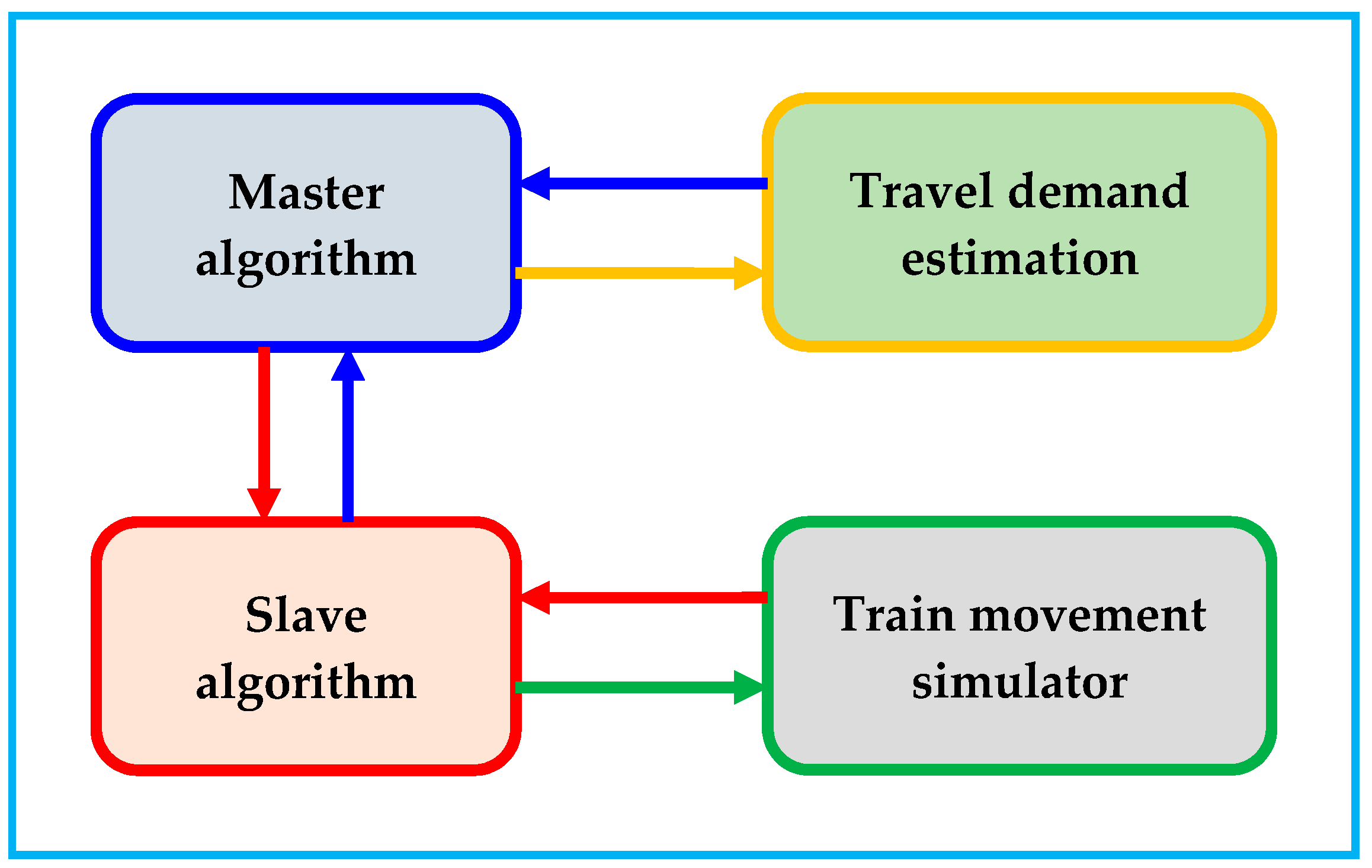
However, the implementation of the master algorithm requires the estimation of travel demand and the solution of the slave algorithm has to be supported by a simulation model of the rail convoy movements. Hence, it is possible to identify two algorithm frameworks:
- Approach 1 (see Figure 2), where running times and energy consumptions are calculated by a train movement simulator at any iteration of the slave algorithm;
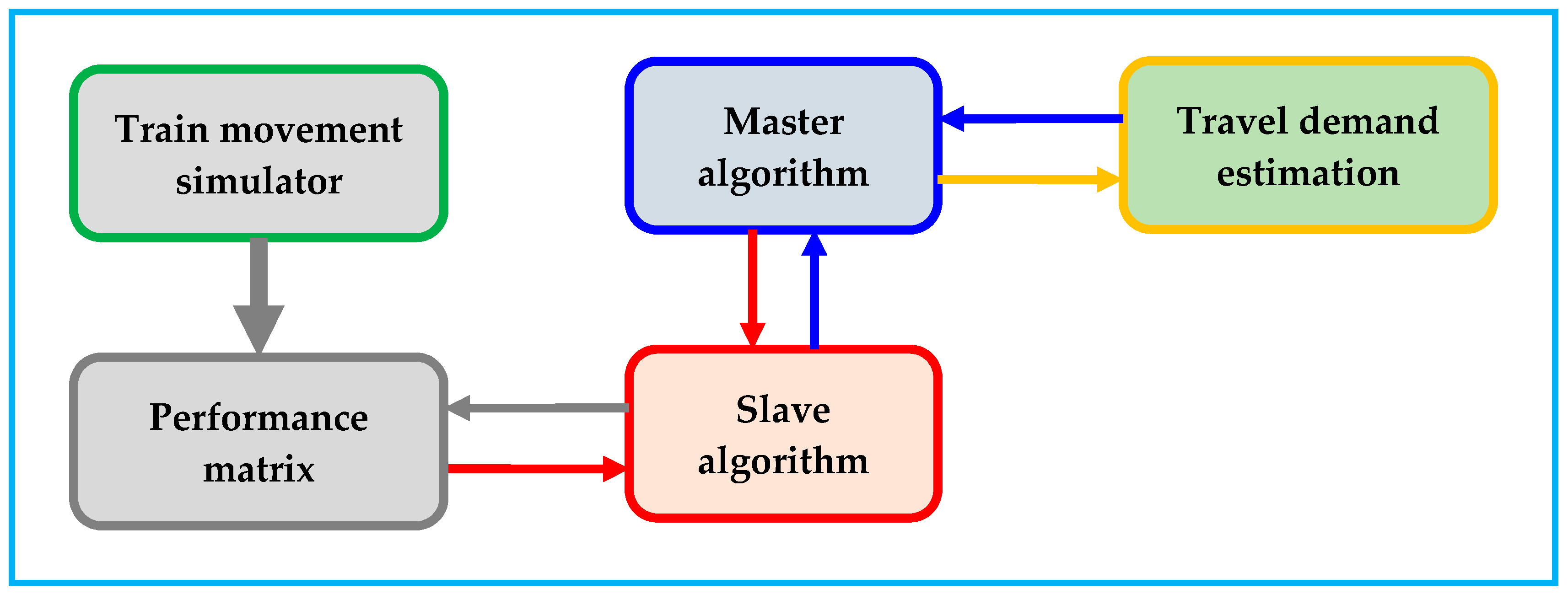
- Approach 2 (see Figure 3), where all feasible speed profiles are preliminary calculated by a train movement simulator and all results in terms of running times and energy consumption are collected in a performance matrix. In this case, the slave algorithm queries the performance matrix without the need of implementing again the train movement simulator.
The adoption of the second approach could increase calculation times in the initial phases of the algorithm (in order to define the performance matrix) but may reduce computing times of the slave algorithm since it does not longer need the train movement simulator.
3.3.1. The Proposed Master Algorithm
Since, as shown in Section 3.2, the upper level seeks for the minimum value of a strictly convex function defined on a non-empty and compact set, it is possible to apply a traditional bisection algorithm, which has been customized to our context as follows:
- Phase 1: Definition of the initial analysis set;
- Phase 2: Partition of the analysis set;
- Phase 3: Objective function calculation;
- Phase 4: Identification of the optimal solution;
- Phase 5: Stop test or definition of a new analysis set.
In the first phase, the initial analysis set is fixed according to constraint (16). The partition of the analysis set (phase 2) is obtained by dividing the analysis set in n values, where n is a positive integer number (i.e., n ∈ Z+) greater than 1. Hence, we obtain n values of as follows:
where is the i-th value of parameter at the k-th iteration; and are the endpoint of the analysis set defined at k-th iteration.
Phase 3 consists in calculating, for any , the corresponding objective function value. Obviously, it is necessary preliminary to implement the slave algorithm in order to obtain the corresponding speed limits (i.e., and ). Then in phase 4, it is identified the which correspond to the minimum objective function value.
The last phase compares the optimal value of the objective function at iteration k with the one obtained in the previous iteration. Obviously, in the case of the first iteration, the comparison cannot be performed, and a new analysis set is generated. However, the comparison verifies if the improvement in objective function is lower than a prefixed threshold, that is:
where is the optimal value of the objective function at k-th iteration; is the prefixed threshold.
If the termination test (38) is verified, the algorithm is stopped; otherwise, a new analysis test is generated, and the algorithm returns to phase 2. The new analysis set is generated as follows:
where is the value of i corresponding to the optimal value of the objective function.
3.3.2. The Proposed Slave Algorithm
Since, as shown in Section 3.2, the lower level seeks for the maximum value of a strictly decreasing function defined on a non-empty and compact set, it is possible to apply a traditional ascendant algorithm, which has been customized to our context as follows:
- Phase 1: Definition of the initial value of the speed limits;
- Phase 2: Calculation of the subsequent Total Running Times;
- Phase 3: Stop test or definition of new speed limits.
Obviously, since running times, as well as speed limits, of the outward trip are independent of the corresponding value of the return trip, the slave algorithm has to be implemented twice: the first time for the outward trip and the second time for the return trip.
In the first phase, the speed limits are fixed equal to the maximum travel speeds reached by rail convoys in the Time Optimal scenario (i.e., and ).
Phase 2 consists in calculating the subsequent Total Running Times (i.e., and ), which in the case of the first iteration correspond to the Time Optimal scenario values (i.e., and ).
The stopping test is based on the verification of constraints (28) and (29). In particular, if these constraints are verified, new speed limits are generated, and the algorithm returns to Step 2. Otherwise, the algorithm terminates, and the final solutions are the speed limits of the previous iteration, that is:
where and are the speed limits at h-th iteration associated, respectively, with the outward trip (ot) and the return trip (rt).
Obviously, since the initial solution (i.e., the solution based on and ) always verifies constraints (28) and (29), the algorithm provides always a valid solution.
Moreover, since speed limits in the real world have to be positive integer numbers, the new values of speed limits may be generated by a simple descendent algorithm as follows:
Finally, if the speed limit reaches the minimum value of allowed speed, that is:
the descendent algorithm terminates without generating a new solution according to Equations (41) and (42). Therefore, although constraints (28) and (29) are still verified, the slave algorithm terminates by adopting the following solutions:
4. Application to a Real Network
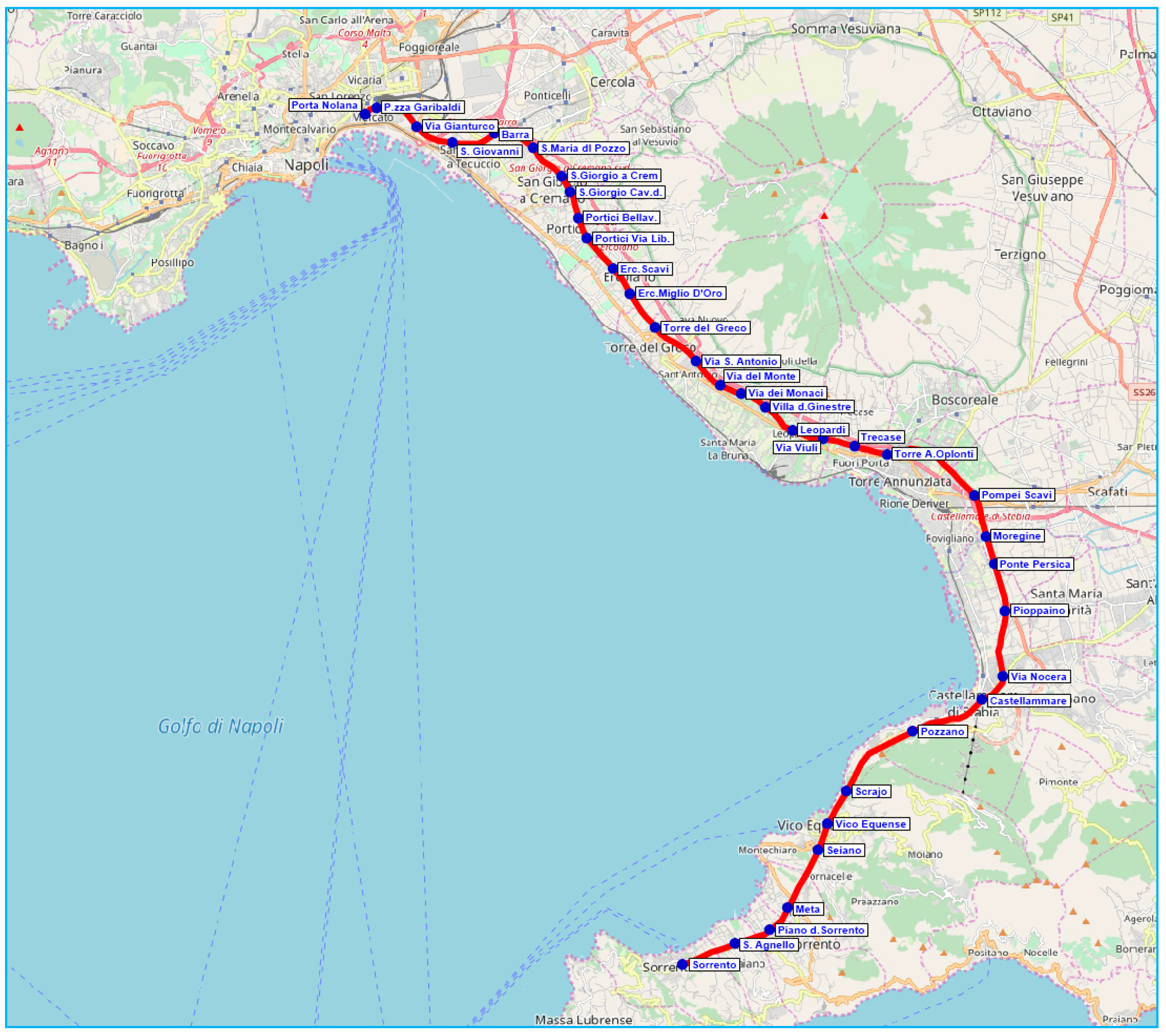
In order to show the utility and the feasibility of the proposed methodology, we applied it to the regional ‘Naples–Sorrento’ rail line serving the metropolitan area of Naples in Italy (see Figure 4).
In particular, although the line has a 17-km single-track section between Moregine and Sorrento (i.e., almost 41% of the line), we assumed the whole line as a double-track line since the doubling has been planned. Moreover, although the terminus in Naples (Napoli Porta Nolana) has 12 tracks, we assumed that only one track is used for the regular service, while the others are adopted as recovery or maintenance tracks. Similarly, the terminus in Sorrento, equipped with 6 tracks, was assumed with only one track adopted for regular service. General details of the line are described in Table 1 in the case of three different confidence levels (i.e., 90th, 95th and 97.5th percentiles) for the buffer time (and therefore cycle time) definition.
Under the above assumptions, the application consisted in identifying some operational schemes and related maximum reductions in energy consumptions, for each one of the three considered confidence levels.
Preliminarily, according to Equation (14), it was necessary to identify feasible operational configurations since the allocation between the outward and return trips may affect the minimum feasible headway of the line. Hence, in Table 2, Table 3 and Table 4, for each headway higher than the minimum infrastructural headway identified in Table 1 (i.e., 6.2 min), we set a certain number of convoys (feasible with limits expressed by Equation (13)) and calculated the term together with thresholds of parameter (expressed by Equation (12)). In particular, by solving the following optimization problem, that is:
subject to:
we are able to determine the value of parameter providing the minimum service headway which has to be compared with the assumed headway. Indeed, whether the identified minimum headway is not greater than the initial value (i.e., assumed headway), the configuration is feasible; otherwise, the assumed configuration is unfeasible since it is based on a headway lower than its minimum. For the sake of clarity, it is worth further making clear that , in Equation (43), is the value of which provides the minimum service headway, thus allowing the identification of feasible configurations complying with Equation (14). However, this is only a preliminary verification step; while, the actual bilevel optimization process is aimed at identifying , i.e., the value of minimizing the objective function (see Equation (15)).
In Table 2, Table 3 and Table 4, feasible configurations are shown in black, while unfeasible configurations are reported in red. Moreover, parameters and represent, respectively, the lower and the upper bound of parameter expressed by Equation (13). Likewise, parameters and represent, respectively, the lower and the upper bound of parameter expressed by Equation (12). However, for any confidence level, we have found 11 feasible solutions.
Finally, for each feasible configuration identified in the previous step, we solved the bilevel optimization problem (15), by determining parameter , i.e., the value of which minimizes objective function . Clearly, the procedure is carried out for any of the considered confidence levels. The travel demand was estimated by means of traditional approaches proposed in the literature (details on the travel demand estimation in the case of the analyzed line may be found in [74,75]. Likewise, we adopted the commercial software OpenTrack [76] as train movement simulator.
In Table 5, Table 6 and Table 7 are shown application results, where and represent variations in passenger on-board time associated, respectively, with the outward trip (ot) and the return trip (rt); and represent variations in energy consumption associated, respectively, with the outward trip (ot) and the return trip (rt); represents the daily variation in energy consumption.
The simulation outcome clearly shows the trade-off phenomenon between the increase in train running time (resulting in an increase in user on-board time) and the reduction in energy consumption. Moreover, as can be seen, the reduction in energy consumption decreases with the increase of the selected percentile. This is due to the fact that higher the confidence level, higher the value of buffer time and, therefore, lower the value of the total layover time to be exploited for compensating the increase in running times resulting from the adoption of eco-driving strategies. Indeed, the maximum reduction occurs in the case of the 90th percentile with a headway of 30 min where decreases in energy consumption are higher than 46%.
Moreover, algorithm performances are shown in Table 8, Table 9 and Table 10, where objective function values and calculation times are indicated for any analyzed scenario. It is worth noting that in terms of calculation times, the approach 1 requires globally 81.88 h for analyzing all scenarios, while the approach 2, which needs 15.25 min for the definition of the performance matrix, requires 18.75 min providing a reduction in computing times equal to 99.62%.
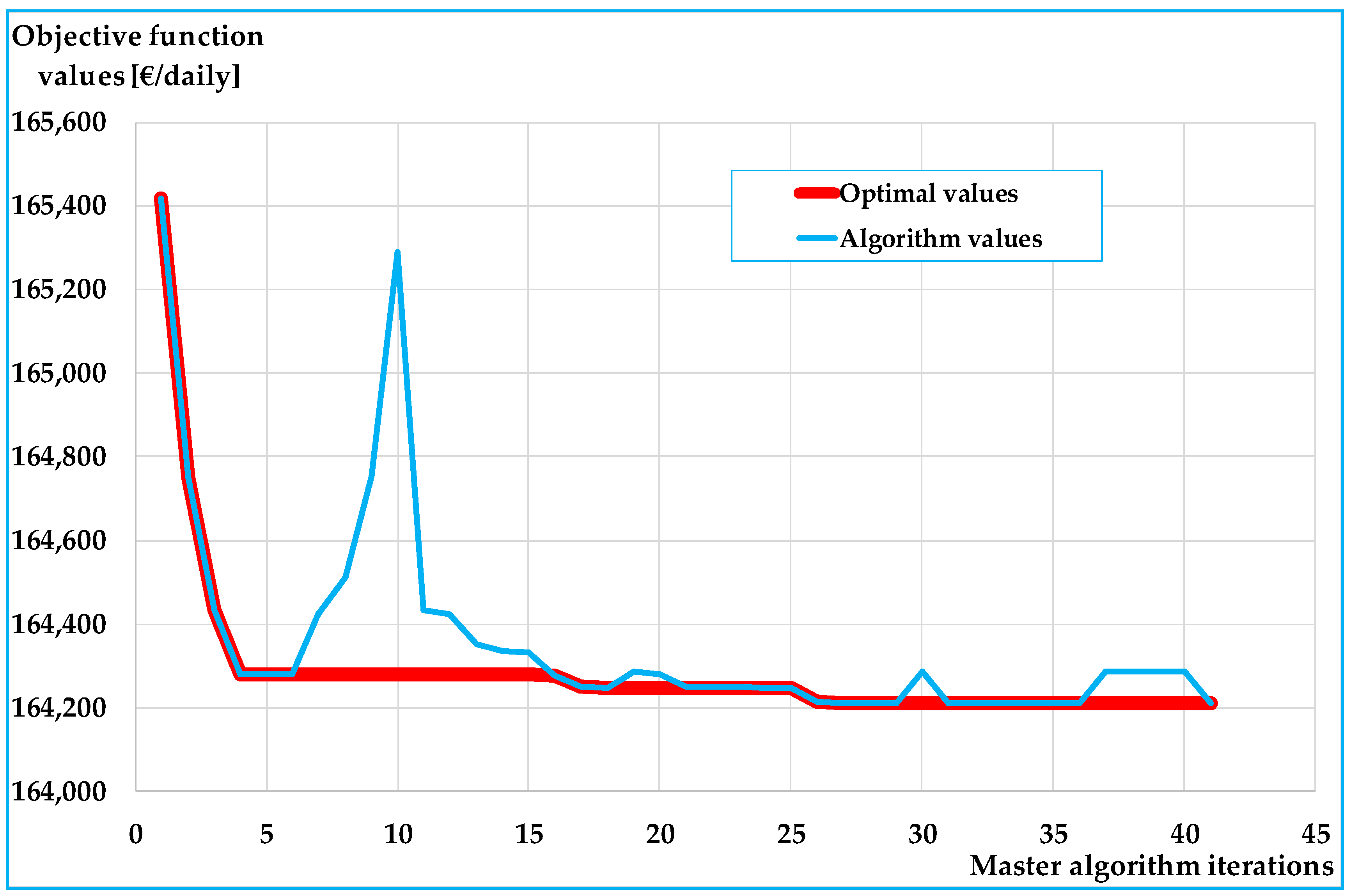
Finally, Figure 5 shows the objective function trend during the master algorithm in the first scenario of 95th percentile (i.e., H = 12.5 min and NC = 13 rail convoys).
5. Conclusions and Research Prospects
Given the key role of energy-saving policies within rail transport management, the proposed approach aims to provide a decision support tool for handling the implementation of eco-driving profiles. The challenge is to reduce energy consumption without prejudicing service stability and by preserving passengers’ satisfaction.
For this purpose, a bilevel analytical framework has been developed which allows to properly estimate all the involved operational factors and the correlations existing among them. Moreover, the allocation of reserve times has been optimized, with the aim of compensating for the increase in train running time generated by such energy-saving measures, and the trade-off between reductions in energy consumption and increases in passenger generalized cost has been investigated.
The presented methodology enables a very realistic assessment of the system, however, as research prospect, we propose to estimate dwell times as flow-dependent factors, rather than as fixed values, so as to derive them with a high degree of accuracy. This could result very useful in an energy-saving perspective; indeed, also eventual time rates exceeding the minimum dwell time required for the boarding/alighting process may be exploited for supporting the implementation of energy-saving strategies preserving service stability.
Moreover, the proposed approach consists in identifying the compromise between energy reductions and travel time increases among solutions which maximize the layover time use (i.e., maximise energy reduction). Hence, as research prospect, we propose to investigate the possibility of developing a different multidimensional optimization problem without the constraint of layover time use maximization. Indeed, greater the freedom degree of the objective function, lower the minimum value achievable.
In order to validate the described methodology, we propose to apply the bilevel optimization problem in the case of a railway network more complex than an isolated railway line. Finally, we suggest investigating effects in terms of solution goodness and/or compromise achievements (between energy reductions and travel time increases) in the case of integration of the slave algorithm with a procedure for determining optimal speed profiles with coasting strategy adoption.
Author Contributions
Conceptualization, L.D.; Data curation, M.B.; Formal analysis, L.D.; Investigation, M.B.; Methodology, L.D.; Validation, L.D. and M.B.; Writing–original draft, L.D. and M.B.; Writing–review and editing, L.D. and M.B.
Funding
This research was partially funded by Federico II University of Naples (Italy), grant number 000009-ALTRO_R-2016-BM “Local Public Transport in Italy”.
Conflicts of Interest
The authors declare no conflicts of interest. The funders had no role in the design of the study; in the collection, analyses, or interpretation of data; in the writing of the manuscript, or in the decision to publish the results.
References
- To, W.M. Centrality of an Urban Rail System. Urban Rail Transit 2015, 1, 249–256. [Google Scholar] [CrossRef] [Green Version]
- D’Acierno, L.; Botte, M. Passengers’ satisfaction in the case of energy-saving strategies: A rail system application. In Proceedings of the 18th IEEE International Conference on Environment and Electrical Engineering (IEEE EEEIC 2018) and 2nd Industrial and Commercial Power Systems Europe (I&CPS 2018), Palermo, Italy, 12–15 June 2018; pp. 795–799. [Google Scholar] [CrossRef]
- Miyatake, M.; Ko, H. Optimization of train speed profile for minimum energy consumption. IEEJ Trans. Electr. Electron. Eng. 2010, 5, 263–269. [Google Scholar] [CrossRef]
- Albrecht, A.; Howlett, P.; Pudney, P.; Vu, X. Energy-efficient train control: From local convexity to global optimization and uniqueness. Automatica 2013, 49, 3072–3078. [Google Scholar] [CrossRef]
- Gallo, M.; Simonelli, F.; De Luca, G.; De Martinis, V. Estimating the effects of energy-efficient driving profiles on railway consumption. In Proceedings of the 15th International Conference on Environment and Electrical Engineering (IEEE EEEIC 2015), Rome, Italy, 10–13 June 2015. [Google Scholar] [CrossRef]
- Steiner, R.; Klohr, M.; Pagiela, S. Energy storage system with ultracaps on board of railway vehicles. In Proceedings of the 12th European Conference on Power Electronics and Applications, Aalborg, Denmark, 2–5 September 2007. [Google Scholar] [CrossRef]
- Miyatake, M.; Matsuda, K. Energy saving speed and charge/discharge control of a railway vehicle with on-board energy storage by means of an optimization model. IEEJ Trans. Electr. Electron. Eng. 2009, 4, 771–778. [Google Scholar] [CrossRef]
- Gao, Z.C.; Chin, C.S.; Toh, W.D.; Chiew, J.; Jia, J. State-of-charge estimation and active cell pack balancing design of lithium battery power system for smart electric vehicle. J. Adv. Transport. 2017, 2017, 6510747. [Google Scholar] [CrossRef]
- Romo, L.; Turner, D.; Ng, L.S.B. Cutting traction power costs with wayside energy storage systems in rail transit systems. In Proceedings of the 2005 ASME/IEEE Joint Rail Conference (ASME/IEEE JRC 2005), Pueblo, CO, USA, 16–18 March 2005. [Google Scholar] [CrossRef]
- Teymourfar, R.; Asaei, B.; Iman-Eini, H.; Nejati Fard, R. Stationary super-capacitor energy storage system to save regenerative braking energy in a metro line. Energy Convers. Manag. 2012, 56, 206–214. [Google Scholar] [CrossRef]
- Ramos, A.; Pena, M.; Fernndez-Cardador, A.; Cucala, A.P. Mathematical programming approach to underground timetabling problem for maximizing time synchronization. In Proceedings of the International Conference on Industrial Engineering and Industrial Management, Madrid, Spain, 5–7 September 2007. [Google Scholar]
- Nasri, A.; Fekri Moghadam, M.; Mokhtari, H. Timetable optimization for maximum usage of regenerative energy of braking in electrical railway systems. In Proceedings of the International Symposium on Power Electronics, Electrical Drives, Automation and Motion (SPEEDAM 2010), Pisa, Italy, 14–16 June 2010. [Google Scholar] [CrossRef]
- Kim, K.M.; Kim, K.T.; Han, M.S. A model and approaches for synchronized energy saving in timetabling. In Proceedings of the 9th World Congress on Railway Research (WCRR 2011), Lille, France, 22–26 May 2011. [Google Scholar]
- Yang, X.; Li, X.; Gao, Z.; Wang, H.; Tang, T. A cooperative scheduling model for timetable optimization in subway systems. IEEE Trans. Intell. Transp. Syst. 2013, 14, 438–447. [Google Scholar] [CrossRef]
- Wong, K.K.; Ho, T.K. Dwell-time and run-time control for DC mass rapid transit railways. IET Electr. Power Appl. 2007, 1, 956–966. [Google Scholar] [CrossRef] [Green Version]
- Canca, D.; Zarzo, A. Design of energy-efficient timetables in two-way railway rapid transit lines. Transp. Res. Part B 2017, 102, 142–161. [Google Scholar] [CrossRef]
- Hu, K.; Wu, J.; Schwanen, T. Differences in energy consumption in electric vehicles: An exploratory real-world study in Beijing. J. Adv. Transp. 2017, 2017, 4695975. [Google Scholar] [CrossRef]
- Keskin, K.; Karamancioglu, A. Energy-efficient train operation using nature-inspired algorithms. J. Adv. Transp. 2017, 2017, 6173795. [Google Scholar] [CrossRef]
- Cornic, D. Efficient recovery of braking energy through a reversible dc substation. In Proceedings of the Electrical Systems for Aircraft, Railway and Ship Propulsion (ESARS 2010), Bologna, Italy, 19–21 October 2010. [Google Scholar] [CrossRef]
- Ibaiondo, H.; Romo, A. Kinetic energy recovery on railway systems with feedback to the grid. In Proceedings of the 14th International Power Electronics and Motion Control Conference (EPE-PEMC 2010), Ohrid, Macedonia, 6–8 September 2010. [Google Scholar]
- Gonzalez-Gil, A.; Palacin, R.; Batty, P. Sustainable urban rail systems: Strategies and technologies for optimal management of regenerative braking energy. Energy Convers. Manag. 2013, 75, 374–388. [Google Scholar] [CrossRef]
- Ghaviha, N.; Campillo, J.; Bohlin, M.; Dahlquist, E. Review of application of energy storage devices in railway transportation. Energy Procedia 2017, 105, 4561–4568. [Google Scholar] [CrossRef]
- Coxon, S.; Chandler, T.; Wilson, E. Testing the efficacy of platform and train passenger boarding, alighting and dispersal through innovative 3d agent-based modelling techniques. Urban Rail Transit 2015, 1, 87–94. [Google Scholar] [CrossRef]
- Pariota, L.; Bifulco, G.N.; Brackstone, M. A linear dynamic model for driving behavior in car following. Transp. Sci. 2015, 50, 1032–1042. [Google Scholar] [CrossRef]
- Teng, J.; Liu, W.-R. Development of a behavior-based passenger flow assignment model for urban rail transit in section interruption circumstance. Urban Rail Transit 2015, 1, 35–46. [Google Scholar] [CrossRef]
- D’Acierno, L.; Placido, A.; Botte, M.; Montella, B. A methodological approach for managing rail disruptions with different perspectives. Int. J. Math. Models Methods Appl. Sci. 2016, 10, 80–86. [Google Scholar]
- D’Acierno, L.; Placido, A.; Botte, M.; Gallo, M.; Montella, B. Defining robust recovery solutions for preserving service quality during rail/metro systems failure. Int. J. Supply Oper. Manag. 2016, 3, 1351–1372. [Google Scholar] [CrossRef]
- Pariota, L.; Bifulco, G.N.; Galante, F.; Montella, A.; Brackstone, M. Longitudinal control behaviour: Analysis and modelling based on experimental surveys in Italy and the UK. Accid. Anal. Prev. 2016, 89, 74–87. [Google Scholar] [CrossRef] [PubMed] [Green Version]
- Cartenì, A.; Pariota, L.; Henke, I. Hedonic value of high-speed rail services: Quantitative analysis of the students’ domestic tourist attractiveness of the main Italian cities. Transp. Res. Part A 2017, 100, 348–365. [Google Scholar] [CrossRef]
- D’Acierno, L.; Botte, M.; Placido, A.; Caropreso, C.; Montella, B. Methodology for determining dwell times consistent with passenger flows in the case of metro services. Urban Rail Transit 2017, 3, 73–89. [Google Scholar] [CrossRef]
- Tang, M.; Hu, Y. Pedestrian simulation in transit stations using agent-based analysis. Urban Rail Transit 2017, 3, 54–60. [Google Scholar] [CrossRef]
- Tang, T.-Q.; Shao, Y.-X.; Chen, L.; Shang, H.-Y. Modeling passengers’ boarding behavior at the platform of high speed railway station. J. Adv. Transp. 2017, 2017, 4073583. [Google Scholar] [CrossRef]
- Yang, S.; Yang, K.; Gao, Z.; Yang, L.; Shi, J. Last-train timetabling under transfer demand uncertainty: Mean-variance model and heuristic solution. J. Adv. Transp. 2017, 2017, 5095021. [Google Scholar] [CrossRef]
- Zhu, W.; Wang, W.; Huang, Z. Estimating train choices of rail transit passengers with real timetable and automatic fare collection data. J. Adv. Transp. 2017, 2017, 5824051. [Google Scholar] [CrossRef]
- D’Acierno, L.; Botte, M.; Montella, B. Assumptions and simulation of passenger behaviour on rail platforms. Int. J. Transp. Dev. Integr. 2018, 2, 123–135. [Google Scholar] [CrossRef]
- Chuang, H.J.; Chen, C.S.; Lin, C.H.; Hsieh, C.H.; Ho, C.Y. Design of optimal coasting speed for saving social cost in mass rapid transit systems. In Proceedings of the 3rd International Conference on Deregulation and Restructuring and Power Technologies–DRPT 2008, Nianjing, China, 6–9 April 2008. [Google Scholar] [CrossRef]
- Yang, L.; Li, K.; Gao, Z.; Li, X. Optimizing trains movement on a railway network. Omega 2012, 40, 619–633. [Google Scholar] [CrossRef]
- Albrecht, T.; Oettich, S. A new integrated approach to dynamic schedule synchronization and energy-saving train control. WIT Trans. Built Environ. 2002, 61, 847–856. [Google Scholar] [CrossRef]
- Lancien, D.; Fontaine, M. Computing train schedules to save energy. Revue General des Chemins de Fer 1981, 100, 679–692. [Google Scholar]
- Li, X.; Lo, H.K. Energy minimization in dynamic train scheduling and control for metro rail operations. Transp. Res. Part B 2014, 70, 269–284. [Google Scholar] [CrossRef]
- Scheepmaker, G.M.; Goverde, R.M.P. The interplay between energy–efficient train control and scheduled running time supplements. J. Rail Transp. Plan. Manag. 2015, 5, 225–239. [Google Scholar] [CrossRef]
- Mathews, J.H.; Fink, K.D. Numerical Methods Using MATLAB, 4th ed.; Pearson Prentice Hall: Upper Saddle River, NJ, USA, 2004; ISBN 978-0130652485. [Google Scholar]
- Fibonacci, L.P. The Book of Squares. An Annotated Translation into Modern English by L. E. Siegler; Academic Press Incorporated: Orlando, FL, USA, 1987; ISBN 978-0126431308. [Google Scholar]
- Sicre, C.; Cucala, P.; Fernández, A.; Jiménez, J.A.; Ribera, I.; Serrano, A. A method to optimise train energy consumption combining manual energy efficient driving and scheduling. WIT Trans. Built Environ. 2010, 114, 549–560. [Google Scholar] [CrossRef] [Green Version]
- Feng, J.; Li, X.; Liu, H.; Gao, X.; Mao, B. Optimizing the energy-efficient metro train timetable and control strategy in off-peak hour with uncertain passenger demands. Energies 2017, 104, 436. [Google Scholar] [CrossRef]
- Acikbas, S.; Soylemez, M.T. Coasting point optimisation for mass rail transit lines using artificial neural networks and genetic algorithms. IET Electr. Power Appl. 2008, 2, 172–182. [Google Scholar] [CrossRef]
- Lukaszewicz, P. Driving techniques and strategies for freight trains. WIT Trans. Built Environ. 2000, 50, 1065–1073. [Google Scholar] [CrossRef]
- Wong, K.K.; Ho, T.K. Coast control for mass rapid transit railways with searching methods. IEE Proc. Electr. Power Appl. 2004, 151, 365–376. [Google Scholar] [CrossRef] [Green Version]
- Carreno, W.C. Efficient Driving of CBTC ATO Operated Trains. Ph.D. Dissertation, Universidad Pontificia Comillas, Madrid, Spain, 2017. [Google Scholar]
- De Cuadra, F.; Fernandez, A.; de Juan, J.; Herrero, M.A. Energy–saving automatic optimisation of train speed commands using direct search techniques. WIT Trans. Built Environ. 1996, 20, 337–346. [Google Scholar] [CrossRef]
- Domínguez, M.; Fernández–Cardador, A.; Cucala, A.P.; Pecharromán, R.R. Energy savings in metropolitan railway substations through regenerative energy recovery and optimal design of ATO speed profiles. IEEE Trans. Autom. Sci. Eng. 2012, 9, 496–504. [Google Scholar] [CrossRef]
- Zhao, N.; Roberts, C.; Hillmansen, S.; Nicholson, G. A multiple train trajectory optimization to minimize energy consumption and delay. IEEE Trans. Intell. Transp. Syst. 2015, 16, 2363–2372. [Google Scholar] [CrossRef]
- Sicre, C.; Cucala, A.P.; Fernandez, A.; Lukaszewicz, P. Modeling and optimizing energy-efficient manual driving on high-speed lines. IEEJ Trans. Electr. Electron. Eng. 2012, 7, 633–640. [Google Scholar] [CrossRef]
- De Martinis, V.; Weidmann, U.A.; Gallo, M. Towards a simulation-based framework for evaluating energy-efficient solutions in train operation. WIT Trans. Built Environ. 2014, 135, 721–732. [Google Scholar] [CrossRef]
- De Martinis, V.; Weidmann, U.A. Definition of energy-efficient speed profiles within rail traffic by means of supply design models. Res. Transp. Econ. 2015, 54, 41–50. [Google Scholar] [CrossRef]
- Corman, F.; D’Ariano, A.; Pacciarelli, D.; Pranzo, M. Evaluation of green wave policy in real-time railway traffic management. Transp. Res. Part C 2009, 17, 607–616. [Google Scholar] [CrossRef]
- Chang, S.C.; Chung, Y.C. From timetabling to train regulation—A new train operation model. Inf. Softw. Technol. 2005, 47, 575–585. [Google Scholar] [CrossRef]
- D’Ariano, A.; Albrecht, T. Running time re-optimization during real-time timetable perturbations. WIT Trans. Built Environ. 2006, 88, 531–540. [Google Scholar] [CrossRef]
- Sheu, J.W.; Lin, W.S. Automatic train regulation with energy saving using dual heuristic programming. IET Electr. Syst. Transp. 2011, 1, 80–89. [Google Scholar] [CrossRef]
- Huang, H.; Li, K.; Schonfeld, P. Real–time energy–saving metro train rescheduling with primary delay identification. PLoS ONE 2018, 13, e0192792. [Google Scholar] [CrossRef] [PubMed]
- Zhang, H.; Li, S.; Yang, L. Real-time optimal train regulation design for metro lines with energy-saving. Comput. Ind. Eng. 2018. forthcoming. [Google Scholar] [CrossRef]
- Howlett, P.; Pudney, P.; Vu, X. Local energy minimization in optimal train control. Automatica 2009, 45, 2692–2698. [Google Scholar] [CrossRef]
- Khmelnitsky, E. On an optimal control problem of train operation. IEEE Trans. Autom. Contr. 2000, 45, 1257–1266. [Google Scholar] [CrossRef]
- Liu, R.; Golovitcher, I. Energy-efficient operation of rail vehicles. Transp. Res. Part A 2003, 37, 917–932. [Google Scholar] [CrossRef]
- Cucala, A.P.; Fernández, A.; Sicre, C.; Domínguez, M. Fuzzy optimal schedule of high speed train operation to minimize energy consumption with uncertain delays and driver’s behavioral response. Eng. Appl. Artif. Intell. 2012, 25, 1548–1557. [Google Scholar] [CrossRef]
- Toletti, A.; De Martinis, V.; Weidmann, U. Energy savings in mixed rail traffic rescheduling: An RCG approach. In Proceedings of the 19th IEEE International Conference on Intelligent Transportation Systems—IEEE ITSC 2016, Rio de Janeiro, Brazil, 1–4 November 2016. [Google Scholar] [CrossRef]
- Tonosaki, Y.; Koizumi, Y.; Tajima, M.; Miyoshi, M.; Takeba, T.; Miyatake, M. Punctual train operation with energy-saving driving advisory system in dense traffic railway. In Proceedings of the IEEE International Conference on Intelligent Rail Transportation—IEEE ICIRT 2016, Birmingham, UK, 23–25 August 2016. [Google Scholar] [CrossRef]
- Feng, X.; Wang, Q.; Liu, Y.; Xu, B.; Liu, H.; Sun, Q. Ensuring a reasonable passenger capacity utilization rate of a train for its sustainably efficient transport. J. Appl. Res. Technol. 2014, 12, 279–288. [Google Scholar] [CrossRef]
- Canca, D. Analysis of the energy-efficient design of railway rapid transit timetables. In Proceedings of the Workshop on Mathematical Models of Optimization for Transportation Planning, Seville, Spain; 2017. [Google Scholar]
- D’Acierno, L.; Botte, M.; Montella, B. An analytical approach for determining reserve times on metro systems. In Proceedings of the 17th IEEE International Conference on Environment and Electrical Engineering (IEEE EEEIC 2017) and 1st Industrial and Commercial Power Systems Europe (I&CPS 2017), Milan, Italy, 6–9 June 2017; pp. 722–727. [Google Scholar] [CrossRef]
- D’Acierno, L.; Botte, M.; Gallo, M.; Montella, B. Defining reserve times for metro systems: An analytical approach. J. Adv. Transp. 2018, 2018, 5983250. [Google Scholar] [CrossRef]
- Wardman, M. Public transport values of time. Transp. Policy 2004, 11, 363–377. [Google Scholar] [CrossRef] [Green Version]
- Cascetta, E. Transportation Systems Analysis: Models and Applications; Springer: New York, NY, USA, 2009; ISBN 978-0-387-75856-5. [Google Scholar]
- Botte, M.; Di Salvo, C.; Caropreso, C.; Montella, B.; D’Acierno, L. Defining economic and environmental feasibility thresholds in the case of rail signalling systems based on satellite technology. In Proceedings of the 16th IEEE International Conference on Environment and Electrical Engineering (IEEE EEEIC 2016), Florence, Italy, 7–10 June 2016; pp. 251–255. [Google Scholar] [CrossRef]
- Caropreso, C.; Di Salvo, C.; Botte, M.; D’Acierno, L. A long-term analysis of passenger flows on a regional rail line. Int. J. Transp. Dev. Integr. 2017, 1, 329–338. [Google Scholar] [CrossRef]
- Nash, A.; Huerlimann, D. Railroad Simulation Using Open-Track. WIT Trans. Built Environ. 2004, 74, 45–54. [Google Scholar] [CrossRef]
Figure 1.
Cumulative distribution of .

Figure 2.
Approach 1 of the solution algorithm.

Figure 3.
Approach 2 of the solution algorithm.

Figure 4.
Regional ‘Naples–Sorrento’ rail line.

Figure 5.
Objective function values.


Table 1.
Main operational parameters of the regional ‘Naples-Sorrento’ rail line.
| Values | ||
|---|---|---|
| Naples-Sorrento Direction | Sorrento-Naples Direction | |
| Total Running Times | 3262 s [54.4 min] | 3220 s [53.7 min] |
| Total Dwell Times | 1080 s [18.0 min] | 1080 s [18.0 min] |
| Inversion times | 180 s [3.0 min] | 180 s [3.0 min] |
| Buffer times [90th percentile] | 225 s [3.8 min] | 228 s [3.8 min] |
| Planned Cycle Time [90th percentile] | 9455 s [157.6 min] | |
| Buffer times [95th percentile] | 252 s [4.2 min] | 253 s [4.2 min] |
| Planned Cycle Time [95th percentile] | 9507 s [158.5 min] | |
| Buffer times [97.5th percentile] | 275 s [4.6 min] | 275 s [4.6 min] |
| Planned Cycle Time [97.5th percentile] | 9552 s [159.2 min] | |
| Minimum headways | 374 s [6.2 min] | 359 s [6.0 min] |
| Travel distance | 42.6 km | 42.6 km |
| Energy consumption in Time Optimal (TO) condition | 621.2 kWh | 564.2 kWh |
Table 2.
Operational schemes in the case of 90th percentile (black = feasible configurations; red = unfeasible configurations).
Table 2.
Operational schemes in the case of 90th percentile (black = feasible configurations; red = unfeasible configurations).
| H [min] | NC | Feasibility | |||||||
|---|---|---|---|---|---|---|---|---|---|
| 6.5 | 25 | 25 | 25 | 4.92 | 45.1% | 55.9% | 48.0% | 12.34 | NO |
| 7.0 | 23 | 23 | 23 | 3.42 | 6.3% | 95.1% | 47.1% | 11.59 | NO |
| 7.5 | 22 | 22 | 22 | 7.42 | 50.1% | 50.6% | 48.7% | 13.59 | NO |
| 8.0 | 20 | 20 | 20 | 2.42 | 0.0% | 100.0% | 45.9% | 11.09 | NO |
| 8.5 | 19 | 19 | 19 | 3.92 | 0.0% | 100.0% | 47.4% | 11.84 | NO |
| 9.0 | 18 | 18 | 18 | 4.42 | 0.0% | 100.0% | 47.7% | 12.09 | NO |
| 9.5 | 17 | 17 | 17 | 3.92 | 0.0% | 100.0% | 47.4% | 11.84 | NO |
| 10.0 | 16 | 17 | 16 | 2.42 | 0.0% | 100.0% | 45.9% | 11.09 | NO |
| 10.0 | 16 | 17 | 17 | 12.42 | 50.1% | 50.3% | 49.2% | 16.09 | NO |
| 10.5 | 16 | 16 | 16 | 10.42 | 35.7% | 64.8% | 49.0% | 15.09 | NO |
| 11.0 | 15 | 15 | 15 | 7.42 | 2.9% | 97.8% | 48.7% | 13.59 | NO |
| 11.5 | 14 | 15 | 14 | 3.42 | 0.0% | 100.0% | 47.1% | 11.59 | NO |
| 11.5 | 14 | 15 | 15 | 14.92 | 48.4% | 52.0% | 49.3% | 17.34 | NO |
| 12.0 | 14 | 14 | 14 | 10.42 | 21.3% | 79.2% | 49.0% | 15.09 | NO |
| 12.5 | 13 | 14 | 13 | 4.92 | 0.0% | 100.0% | 48.0% | 12.34 | YES |
| 12.5 | 13 | 14 | 14 | 17.42 | 50.0% | 50.2% | 49.4% | 18.59 | NO |
| 13.0 | 13 | 13 | 13 | 11.42 | 19.4% | 81.0% | 49.1% | 15.59 | NO |
| 13.5 | 12 | 13 | 12 | 4.42 | 0.0% | 100.0% | 47.7% | 12.09 | YES |
| 13.5 | 12 | 13 | 13 | 17.92 | 45.9% | 54.4% | 49.4% | 18.84 | NO |
| 14.0 | 12 | 12 | 12 | 10.42 | 2.1% | 98.4% | 49.0% | 15.09 | NO |
| 14.5 | 11 | 12 | 11 | 1.92 | 0.0% | 100.0% | 44.8% | 10.84 | YES |
| 14.5 | 11 | 12 | 12 | 16.42 | 34.8% | 65.5% | 49.4% | 18.09 | NO |
| 15.0 | 11 | 12 | 11 | 7.42 | 0.0% | 100.0% | 48.7% | 13.59 | YES |
| 15.0 | 11 | 12 | 12 | 22.42 | 50.0% | 50.2% | 49.6% | 21.09 | NO |
| 16.0 | 10 | 11 | 10 | 2.42 | 0.0% | 100.0% | 45.9% | 11.09 | YES |
| 16.0 | 10 | 11 | 11 | 18.42 | 33.8% | 66.5% | 49.5% | 19.09 | NO |
| 17.0 | 10 | 10 | 10 | 12.42 | 0.0% | 100.0% | 49.2% | 16.09 | YES |
| 18.0 | 9 | 10 | 9 | 4.42 | 0.0% | 100.0% | 47.7% | 12.09 | YES |
| 18.0 | 9 | 10 | 10 | 22.42 | 36.7% | 63.6% | 49.6% | 21.09 | NO |
| 19.0 | 9 | 9 | 9 | 13.42 | 0.0% | 100.0% | 49.3% | 16.59 | YES |
| 20.0 | 8 | 9 | 8 | 2.42 | 0.0% | 100.0% | 45.9% | 11.09 | YES |
| 20.0 | 8 | 9 | 9 | 22.42 | 27.7% | 72.5% | 49.6% | 21.09 | NO |
| 25.0 | 7 | 8 | 7 | 17.42 | 0.0% | 100.0% | 49.4% | 18.59 | YES |
| 25.0 | 7 | 8 | 8 | 42.42 | 50.0% | 50.1% | 49.8% | 31.09 | NO |
| 30.0 | 6 | 7 | 6 | 22.42 | 0.0% | 100.0% | 49.6% | 21.09 | YES |
| 30.0 | 6 | 7 | 7 | 52.42 | 50.0% | 50.1% | 49.8% | 36.09 | NO |
Table 3.
Operational schemes in the case of 95th percentile (black = feasible configurations; red = unfeasible configurations).
Table 3.
Operational schemes in the case of 95th percentile (black = feasible configurations; red = unfeasible configurations).
| H [min] | NC | Feasibility | |||||||
|---|---|---|---|---|---|---|---|---|---|
| 6.5 | 25 | 25 | 25 | 4.05 | 43.6% | 56.8% | 47.1% | 12.34 | NO |
| 7.0 | 23 | 23 | 23 | 2.55 | 0.0% | 100.0% | 45.4% | 11.59 | NO |
| 7.5 | 22 | 22 | 22 | 6.55 | 49.9% | 50.4% | 48.2% | 13.59 | NO |
| 8.0 | 20 | 20 | 20 | 1.55 | 0.0% | 100.0% | 42.5% | 11.09 | NO |
| 8.5 | 19 | 19 | 19 | 3.05 | 0.0% | 100.0% | 46.2% | 11.84 | NO |
| 9.0 | 18 | 18 | 18 | 3.55 | 0.0% | 100.0% | 46.7% | 12.09 | NO |
| 9.5 | 17 | 17 | 17 | 3.05 | 0.0% | 100.0% | 46.2% | 11.84 | NO |
| 10.0 | 16 | 17 | 16 | 1.55 | 0.0% | 100.0% | 42.5% | 11.09 | NO |
| 10.0 | 16 | 17 | 17 | 11.55 | 49.9% | 50.2% | 49.0% | 16.09 | NO |
| 10.5 | 16 | 16 | 16 | 9.55 | 34.2% | 66.0% | 48.8% | 15.09 | NO |
| 11.0 | 15 | 15 | 15 | 6.55 | 0.0% | 100.0% | 48.2% | 13.59 | NO |
| 11.5 | 14 | 15 | 14 | 2.55 | 0.0% | 100.0% | 45.4% | 11.59 | NO |
| 11.5 | 14 | 15 | 15 | 14.05 | 48.2% | 52.0% | 49.2% | 17.34 | NO |
| 12.0 | 14 | 14 | 14 | 9.55 | 18.5% | 81.7% | 48.8% | 15.09 | NO |
| 12.5 | 13 | 14 | 13 | 4.05 | 0.0% | 100.0% | 47.1% | 12.34 | YES |
| 12.5 | 13 | 14 | 14 | 16.55 | 49.9% | 50.2% | 49.3% | 18.59 | NO |
| 13.0 | 13 | 13 | 13 | 10.55 | 16.7% | 83.4% | 48.9% | 15.59 | NO |
| 13.5 | 12 | 13 | 12 | 3.55 | 0.0% | 100.0% | 46.7% | 12.09 | YES |
| 13.5 | 12 | 13 | 13 | 17.05 | 45.6% | 54.5% | 49.3% | 18.84 | NO |
| 14.0 | 12 | 12 | 12 | 9.55 | 0.0% | 100.0% | 48.8% | 15.09 | NO |
| 14.5 | 11 | 12 | 11 | 1.05 | 0.0% | 100.0% | 38.9% | 10.84 | YES |
| 14.5 | 11 | 12 | 12 | 15.55 | 33.9% | 66.2% | 49.2% | 18.09 | NO |
| 15.0 | 11 | 12 | 11 | 6.55 | 0.0% | 100.0% | 48.2% | 13.59 | YES |
| 15.0 | 11 | 12 | 12 | 21.55 | 50.0% | 50.1% | 49.5% | 21.09 | NO |
| 16.0 | 10 | 11 | 10 | 1.55 | 0.0% | 100.0% | 42.5% | 11.09 | YES |
| 16.0 | 10 | 11 | 11 | 17.55 | 32.9% | 67.2% | 49.3% | 19.09 | NO |
| 17.0 | 10 | 10 | 10 | 11.55 | 0.0% | 100.0% | 49.0% | 16.09 | YES |
| 18.0 | 9 | 10 | 9 | 3.55 | 0.0% | 100.0% | 46.7% | 12.09 | YES |
| 18.0 | 9 | 10 | 10 | 21.55 | 36.0% | 64.0% | 49.5% | 21.09 | NO |
| 19.0 | 9 | 9 | 9 | 12.55 | 0.0% | 100.0% | 49.1% | 16.59 | YES |
| 20.0 | 8 | 9 | 8 | 1.55 | 0.0% | 100.0% | 42.5% | 11.09 | YES |
| 20.0 | 8 | 9 | 9 | 21.55 | 26.8% | 73.3% | 49.5% | 21.09 | NO |
| 25.0 | 7 | 8 | 7 | 16.55 | 0.0% | 100.0% | 49.3% | 18.59 | YES |
| 25.0 | 7 | 8 | 8 | 41.55 | 50.0% | 50.1% | 49.7% | 31.09 | NO |
| 30.0 | 6 | 7 | 6 | 21.55 | 0.0% | 100.0% | 49.5% | 21.09 | YES |
| 30.0 | 6 | 7 | 7 | 51.55 | 50.0% | 50.0% | 49.8% | 36.09 | NO |
Table 4.
Operational schemes in the case of 97.5th percentile (black = feasible configurations; red = unfeasible configurations).
Table 4.
Operational schemes in the case of 97.5th percentile (black = feasible configurations; red = unfeasible configurations).
| H [min] | NC | Feasibility | |||||||
|---|---|---|---|---|---|---|---|---|---|
| 6.5 | 25 | 25 | 25 | 3.30 | 41.9% | 58.1% | 46.2% | 12.34 | NO |
| 7.0 | 23 | 23 | 23 | 1.80 | 0.0% | 100.0% | 43.1% | 11.59 | NO |
| 7.5 | 22 | 22 | 22 | 5.80 | 49.7% | 50.3% | 47.8% | 13.59 | NO |
| 8.0 | 20 | 20 | 20 | 0.80 | 0.0% | 100.0% | 34.4% | 11.09 | NO |
| 8.5 | 19 | 19 | 19 | 2.30 | 0.0% | 100.0% | 44.6% | 11.84 | NO |
| 9.0 | 18 | 18 | 18 | 2.80 | 0.0% | 100.0% | 45.5% | 12.09 | NO |
| 9.5 | 17 | 17 | 17 | 2.30 | 0.0% | 100.0% | 44.6% | 11.84 | NO |
| 10.0 | 16 | 17 | 16 | 0.80 | 0.0% | 100.0% | 34.4% | 11.09 | NO |
| 10.0 | 16 | 17 | 17 | 10.80 | 49.8% | 50.2% | 48.8% | 16.09 | NO |
| 10.5 | 16 | 16 | 16 | 8.80 | 32.8% | 67.2% | 48.6% | 15.09 | NO |
| 11.0 | 15 | 15 | 15 | 5.80 | 0.0% | 100.0% | 47.8% | 13.59 | NO |
| 11.5 | 14 | 15 | 14 | 1.80 | 0.0% | 100.0% | 43.1% | 11.59 | NO |
| 11.5 | 14 | 15 | 15 | 13.30 | 48.0% | 52.0% | 49.1% | 17.34 | NO |
| 12.0 | 14 | 14 | 14 | 8.80 | 15.7% | 84.3% | 48.6% | 15.09 | NO |
| 12.5 | 13 | 14 | 13 | 3.30 | 0.0% | 100.0% | 46.2% | 12.34 | YES |
| 12.5 | 13 | 14 | 14 | 15.80 | 49.9% | 50.1% | 49.2% | 18.59 | NO |
| 13.0 | 13 | 13 | 13 | 9.80 | 14.1% | 85.9% | 48.7% | 15.59 | NO |
| 13.5 | 12 | 13 | 12 | 2.80 | 0.0% | 100.0% | 45.5% | 12.09 | YES |
| 13.5 | 12 | 13 | 13 | 16.30 | 45.3% | 54.7% | 49.2% | 18.84 | NO |
| 14.0 | 12 | 12 | 12 | 8.80 | 0.0% | 100.0% | 48.6% | 15.09 | NO |
| 14.5 | 11 | 12 | 11 | 0.30 | 0.0% | 100.0% | 8.3% | 10.84 | YES |
| 14.5 | 11 | 12 | 12 | 14.80 | 33.0% | 67.0% | 49.2% | 18.09 | NO |
| 15.0 | 11 | 12 | 11 | 5.80 | 0.0% | 100.0% | 47.8% | 13.59 | YES |
| 15.0 | 11 | 12 | 12 | 20.80 | 49.9% | 50.1% | 49.4% | 21.09 | NO |
| 16.0 | 10 | 11 | 10 | 0.80 | 0.0% | 100.0% | 34.4% | 11.09 | YES |
| 16.0 | 10 | 11 | 11 | 16.80 | 32.0% | 68.0% | 49.3% | 19.09 | NO |
| 17.0 | 10 | 10 | 10 | 10.80 | 0.0% | 100.0% | 48.8% | 16.09 | YES |
| 18.0 | 9 | 10 | 9 | 2.80 | 0.0% | 100.0% | 45.5% | 12.09 | YES |
| 18.0 | 9 | 10 | 10 | 20.80 | 35.5% | 64.5% | 49.4% | 21.09 | NO |
| 19.0 | 9 | 9 | 9 | 11.80 | 0.0% | 100.0% | 48.9% | 16.59 | YES |
| 20.0 | 8 | 9 | 8 | 0.80 | 0.0% | 100.0% | 34.4% | 11.09 | YES |
| 20.0 | 8 | 9 | 9 | 20.80 | 25.9% | 74.1% | 49.4% | 21.09 | NO |
| 25.0 | 7 | 8 | 7 | 15.80 | 0.0% | 100.0% | 49.2% | 18.59 | YES |
| 25.0 | 7 | 8 | 8 | 40.80 | 50.0% | 50.0% | 49.7% | 31.09 | NO |
| 30.0 | 6 | 7 | 6 | 20.80 | 0.0% | 100.0% | 49.4% | 21.09 | YES |
| 30.0 | 6 | 7 | 7 | 50.80 | 50.0% | 50.0% | 49.8% | 36.09 | NO |
Table 5.
Energy saving optimization in the case of 90th percentile.
| H [min] | NC | [km/h] | [km/h] | [s] | [s] | [kWh] | [kWh] | [kWh] | Reduction in Energy Consumption | |
|---|---|---|---|---|---|---|---|---|---|---|
| 12.5 | 13 | 49.52% | 67 | 68 | 129 | 147 | −136.8 | −139.8 | −21,019 | −23.33% |
| 13.5 | 12 | 37.04% | 70 | 67 | 87 | 163 | −110.9 | −149.1 | −18,315 | −21.91% |
| 14.5 | 11 | 43.21% | 74 | 76 | 49 | 65 | −80.6 | −80.3 | −10,544 | −13.58% |
| 15.0 | 11 | 58.71% | 61 | 66 | 241 | 180 | −186.5 | −156.2 | −21,587 | −28.91% |
| 16.0 | 10 | 34.57% | 74 | 73 | 49 | 90 | −80.6 | −103.5 | −10,943 | −15.51% |
| 17.0 | 10 | 38.55% | 60 | 55 | 263 | 434 | −193.0 | −242.9 | −24,166 | −36.72% |
| 18.0 | 9 | 37.04% | 70 | 67 | 87 | 163 | −110.9 | −149.1 | −13,783 | −21.94% |
| 19.0 | 9 | 58.30% | 54 | 59 | 436 | 320 | −237.7 | −211.8 | −22,478 | −37.93% |
| 20.0 | 8 | 33.33% | 75 | 73 | 41 | 90 | −73.5 | −103.5 | −8,389 | −14.89% |
| 25.0 | 7 | 55.56% | 51 | 55 | 542 | 434 | −261.6 | −242.9 | −19,172 | −42.56% |
| 30.0 | 6 | 46.96% | 50 | 49 | 588 | 668 | −265.2 | −283.8 | −17,285 | −46.26% |
Table 6.
Energy saving optimization in the case of 95th percentile.
| H [min] | NC | [km/h] | [km/h] | [s] | [s] | [kWh] | [kWh] | [kWh] | Reduction in Energy Consumption | |
|---|---|---|---|---|---|---|---|---|---|---|
| 12.5 | 13 | 41.43% | 70 | 69 | 87 | 134 | −110.9 | −132.8 | −18,523 | −20.56% |
| 13.5 | 12 | 39.51% | 71 | 70 | 79 | 123 | −103.8 | −124.2 | −16,064 | −19.22% |
| 14.5 | 11 | 54.32% | 77 | 82 | 29 | 27 | −61.8 | −42.9 | −6869 | −8.84% |
| 15.0 | 11 | 61.32% | 62 | 68 | 218 | 147 | −178.7 | −139.8 | −20,067 | −26.87% |
| 16.0 | 10 | 27.85% | 79 | 76 | 21 | 65 | −48.8 | −80.3 | −7669 | −10.87% |
| 17.0 | 10 | 34.57% | 62 | 55 | 218 | 434 | −178.7 | −242.9 | −23,369 | −35.51% |
| 18.0 | 9 | 45.68% | 70 | 71 | 87 | 113 | −110.9 | −118.2 | −12,144 | −19.33% |
| 19.0 | 9 | 66.67% | 53 | 63 | 473 | 233 | −247.8 | −179.8 | −21,378 | −36.07% |
| 20.0 | 8 | 27.85% | 79 | 76 | 21 | 65 | −48.8 | −80.3 | −6119 | −10.86% |
| 25.0 | 7 | 84.22% | 46 | 68 | 780 | 147 | −296.2 | −139.8 | −16,567 | −36.78% |
| 30.0 | 6 | 33.33% | 55 | 46 | 402 | 814 | −232.5 | −304.9 | −16,892 | −45.20% |
Table 7.
Energy saving optimization in the case of 97.5th percentile.
| H [min] | NC | [km/h] | [km/h] | [sec] | [sec] | [kWh] | [kWh] | [kWh] | Reduction in Energy Consumption | |
|---|---|---|---|---|---|---|---|---|---|---|
| 12.5 | 13 | 50.89% | 70 | 73 | 87 | 90 | −110.9 | −103.5 | −16,294 | −18.09% |
| 13.5 | 12 | 37.04% | 73 | 72 | 59 | 100 | −87.8 | −108.2 | −13,809 | −16.52% |
| 14.5 | 11 | 100% | 80 | 90 | 18 | 0 | −41.0 | 0.0 | −2708 | −3.49% |
| 15.0 | 11 | 67.90% | 62 | 72 | 218 | 100 | −178.7 | −108.2 | −18,077 | −24.21% |
| 16.0 | 10 | 6.17% | 88 | 79 | 2 | 43 | −5.2 | −61.3 | −3932 | −5.57% |
| 17.0 | 10 | 41.98% | 60 | 58 | 263 | 350 | −193.0 | −222.0 | −23,018 | −34.97% |
| 18.0 | 9 | 60.08% | 70 | 76 | 87 | 65 | −110.9 | −80.3 | −10,136 | −16.13% |
| 19.0 | 9 | 48.42% | 58 | 58 | 315 | 350 | −211.2 | −222.0 | −21,661 | −36.55% |
| 20.0 | 8 | 6.17% | 88 | 79 | 2 | 43 | −5.2 | −61.3 | −3133 | −5.56% |
| 25.0 | 7 | 66.67% | 50 | 60 | 588 | 298 | −265.2 | −204.0 | −17,830 | −39.58% |
| 30.0 | 6 | 43.21% | 52 | 49 | 507 | 668 | −251.3 | −283.8 | −16,839 | −45.06% |
Table 8.
Solution algorithm performance in the case of 90th percentile.
| H [min] | NC | [€/Daily] | [€/Daily] | [€/Daily] | Master Algorithm Iterations | Slave Algorithm Iterations | Approach 1 Computing Times [h] | Approach 2 Computing Times [s] | |
|---|---|---|---|---|---|---|---|---|---|
| 12.5 | 13 | 49.52% | 13,814 | 150,511 | 164,325 | 31 | 1473 | 2.70 | 13.71 |
| 13.5 | 12 | 37.04% | 13,056 | 154,000 | 167,056 | 21 | 938 | 1.72 | 8.00 |
| 14.5 | 11 | 43.21% | 13,425 | 156,664 | 170,089 | 31 | 995 | 1.77 | 8.99 |
| 15.0 | 11 | 58.71% | 10,618 | 161,367 | 171,985 | 31 | 1724 | 3.21 | 8.04 |
| 16.0 | 10 | 34.57% | 11,923 | 162,469 | 174,392 | 21 | 358 | 1.30 | 5.33 |
| 17.0 | 10 | 38.55% | 8330 | 171,736 | 180,066 | 31 | 1074 | 3.98 | 6.44 |
| 18.0 | 9 | 37.04% | 9808 | 171,797 | 181,606 | 21 | 479 | 1.72 | 4.57 |
| 19.0 | 9 | 58.30% | 7358 | 180,661 | 188,019 | 31 | 2131 | 4.08 | 5.62 |
| 20.0 | 8 | 33.33% | 9589 | 177,513 | 187,102 | 21 | 727 | 1.30 | 3.82 |
| 25.0 | 7 | 55.56% | 5174 | 206,508 | 211,683 | 21 | 1563 | 3.03 | 2.89 |
| 30.0 | 6 | 46.96% | 4016 | 227,726 | 231,743 | 41 | 3430 | 6.72 | 3.60 |
Table 9.
Solution algorithm performance in the case of 95th percentile.
| H [min] | NC | [€/Daily] | [€/Daily] | [€/Daily] | Master Algorithm Iterations | Slave Algorithm Iterations | Approach 1 Computing Times [h] | Approach 2 Computing Times [s] | |
|---|---|---|---|---|---|---|---|---|---|
| 12.5 | 13 | 41.43% | 14,313 | 149,897 | 164,210 | 41 | 1817 | 3.31 | 15.49 |
| 13.5 | 12 | 39.51% | 13,507 | 153,461 | 166,968 | 21 | 859 | 1.56 | 7.60 |
| 14.5 | 11 | 54.32% | 14,160 | 156,033 | 170,194 | 21 | 507 | 0.89 | 6.77 |
| 15.0 | 11 | 61.32% | 10,922 | 160,751 | 171,673 | 31 | 1627 | 3.02 | 8.93 |
| 16.0 | 10 | 27.85% | 12,578 | 161,868 | 174,446 | 31 | 877 | 1.55 | 8.02 |
| 17.0 | 10 | 34.57% | 8490 | 171,232 | 179,722 | 21 | 1347 | 2.56 | 5.26 |
| 18.0 | 9 | 45.68% | 10,136 | 171,217 | 181,353 | 21 | 861 | 1.56 | 4.79 |
| 19.0 | 9 | 66.67% | 7578 | 180,084 | 187,663 | 21 | 1383 | 2.64 | 4.34 |
| 20.0 | 8 | 27.85% | 10,043 | 176,984 | 187,027 | 31 | 877 | 1.55 | 5.24 |
| 25.0 | 7 | 84.22% | 5696 | 205,669 | 211,365 | 31 | 2197 | 4.24 | 3.84 |
| 30.0 | 6 | 33.33% | 4095 | 227,409 | 231,504 | 21 | 1676 | 3.28 | 2.32 |
Table 10.
Solution algorithm performance in the case of 97.5th percentile.
| H [min] | NC | [€/Daily] | [€/Daily] | [€/Daily] | Master Algorithm Iterations | Slave Algorithm Iterations | Approach 1 Computing Times [h] | Approach 2 Computing Times [s] | |
|---|---|---|---|---|---|---|---|---|---|
| 12.5 | 13 | 50.89% | 14,759 | 149,409 | 164,168 | 31 | 1251 | 2.26 | 11.81 |
| 13.5 | 12 | 37.04% | 13,958 | 152,995 | 166,953 | 21 | 778 | 1.40 | 7.54 |
| 14.5 | 11 | 100% | 14,992 | 155,634 | 170,626 | 21 | 277 | 0.48 | 6.33 |
| 15.0 | 11 | 67.90% | 11,320 | 160,227 | 171,547 | 21 | 1028 | 1.90 | 6.25 |
| 16.0 | 10 | 6.17% | 13,325 | 161,469 | 174,795 | 31 | 562 | 0.98 | 7.30 |
| 17.0 | 10 | 41.98% | 8560 | 170,801 | 179,361 | 21 | 1315 | 2.49 | 4.89 |
| 18.0 | 9 | 60.08% | 10,538 | 170,657 | 181,195 | 31 | 1155 | 2.08 | 5.92 |
| 19.0 | 9 | 48.42% | 7522 | 179,699 | 187,221 | 31 | 2051 | 3.90 | 5.38 |
| 20.0 | 8 | 6.17% | 10,640 | 176,585 | 187,225 | 31 | 562 | 0.98 | 5.03 |
| 25.0 | 7 | 66.67% | 5443 | 205,414 | 210,857 | 21 | 1503 | 2.90 | 2.87 |
| 30.0 | 6 | 43.21% | 4106 | 226,873 | 230,979 | 31 | 2509 | 4.90 | 2.89 |
© 2018 by the authors. Licensee MDPI, Basel, Switzerland. This article is an open access article distributed under the terms and conditions of the Creative Commons Attribution (CC BY) license (http://creativecommons.org/licenses/by/4.0/).
Share and Cite
MDPI and ACS Style
D’Acierno, L.; Botte, M. A Passenger-Oriented Optimization Model for Implementing Energy-Saving Strategies in Railway Contexts. Energies 2018, 11, 2946. https://doi.org/10.3390/en11112946
AMA Style
D’Acierno L, Botte M. A Passenger-Oriented Optimization Model for Implementing Energy-Saving Strategies in Railway Contexts. Energies. 2018; 11(11):2946. https://doi.org/10.3390/en11112946
Chicago/Turabian StyleD’Acierno, Luca, and Marilisa Botte. 2018. "A Passenger-Oriented Optimization Model for Implementing Energy-Saving Strategies in Railway Contexts" Energies 11, no. 11: 2946. https://doi.org/10.3390/en11112946
Note that from the first issue of 2016, this journal uses article numbers instead of page numbers. See further details here.