OBS Data Analysis to Quantify Gas Hydrate and Free Gas in the South Shetland Margin (Antarctica)
by
 , ,
, ,
Sha Song
1,*, 
Umberta Tinivella
2,
Michela Giustiniani
2 ,
,
Sunny Singhroha
3,
Stefan Bünz
3 and
Giorgio Cassiani
1 1
Department of Geosciences, University of Padova, Via Gradenigo 6, 35131 Padova, Italy
2
Istituto Nazionale di Oceanografia e di Geofisica Sperimentale—OGS, 34010 Sgonico, Italy
3
CAGE—Centre for Arctic Gas Hydrate, Environment and Climate, Department of Geosciences, UiT The Arctic University of Norway, Dramsveien 201, 9010 Tromsø, Norway
*
Author to whom correspondence should be addressed.
Energies 2018, 11(12), 3290; https://doi.org/10.3390/en11123290
Submission received: 6 October 2018
/
Revised: 13 November 2018
/
Accepted: 21 November 2018
/
Published: 25 November 2018
Abstract
:The presence of a gas hydrate reservoir and free gas layer along the South Shetland margin (offshore Antarctic Peninsula) has been well documented in recent years. In order to better characterize gas hydrate reservoirs, with a particular focus on the quantification of gas hydrate and free gas and the petrophysical properties of the subsurface, we performed travel time inversion of ocean-bottom seismometer data in order to obtain detailed P- and S-wave velocity estimates of the sediments. The P-wave velocity field is determined by the inversion of P-wave refractions and reflections, while the S-wave velocity field is obtained from converted-wave reflections received on the horizontal components of ocean-bottom seismometer data. The resulting velocity fields are used to estimate gas hydrate and free gas concentrations using a modified Biot-Geertsma-Smit theory. The results show that hydrate concentration ranges from 10% to 15% of total volume and free gas concentration is approximately 0.3% to 0.8% of total volume. The comparison of Poisson’s ratio with previous studies in this area indicates that the gas hydrate reservoir shows no significant regional variations.
1. Introduction
Gas hydrates are ice-like crystalline solids composed of water and low-molecular-weight gases (mostly methane), which form under conditions of high pressure, low temperature, and sufficient gas concentration [1]. Hydrates are widespread in the shallow marine sediments along continental margins and in permafrost areas [2]. Gas hydrates in the marine sediments have commonly been inferred on the basis of seismic reflection profiles from the presence of a so-called bottom simulating reflection (BSR) that marks the base of the gas hydrate stability zone [3]. A BSR is generated due to the strong impedance contrast between hydrate-bearing sediments above and underlying free gas-bearing sediments. During the last few decades, much effort has been expended on the study of gas hydrates because of their economic potential as a future energy source [4,5] and their potential role in geohazards [6,7,8] and global climate change [9,10,11,12,13,14,15].
In the majority of situations, where no direct measurements are available, the analysis of seismic velocity provides an efficient way to identify and characterize the distribution of gas hydrates and free gas in marine sediments [7,16,17,18,19,20]. Gas hydrate-bearing sediments show higher P-wave velocity (VP) compared to water-saturated sediments whereas the presence of free gas reduces the P-wave velocity with respect to water-saturated sediments [17]. The effect of gas hydrates on S-wave velocity (VS) is different because it depends on the micro-scale distribution of hydrates within the sediments, i.e., as pore fluid components or cementing grain contacts (e.g., References [20,21,22,23]). Therefore, the measurement of S-wave velocity is crucial, and it can help to understand the distribution of gas hydrates within the pore space and provide additional constraints in estimating hydrate concentration [3,12,23]. The analysis of shear waves can be achieved by deploying multi-component ocean-bottom seismometer (OBS) on the seafloor which allows recording of converted PS-wave reflections, in addition to wide-angle P-wave reflections and refractions.
OBS data have been used successfully in the characterization of gas hydrate reservoirs by combined analysis of P- and S-waves, and the importance of S-wave velocity has been pointed out [23,24,25]. In the South Shetland margin (offshore Antarctic Peninsula), very few studies have been performed to estimate hydrate concentration utilizing OBS data. For example, in the last 20 years, only one OBS deployed during the 1996/97 cruise was analyzed by Reference [3]: the P-wave velocity structure and Poisson’s ratio in the marine sediments were estimated by travel time inversion of reflections and refractions and then were used to quantify the amounts of gas hydrate and free gas. The Poisson’s ratio obtained from the analysis of this OBS has been used by several authors to evaluate the shear modulus of sediment in the same area [26,27,28].
The occurrence of a potential gas hydrate reservoir has been demonstrated from the analysis of seismic data acquired during three Italian Antarctic cruises in 1989/1990, 1996/1997, and 2003/2004, onboard the R/V OGS Explora (e.g., References [3,29,30,31]). The South Shetland margin is located in the northeastern tip of the Pacific margin of the Antarctic Peninsula, which is characterized by the subduction of the Antarctic and the former Phoenix plates beneath the South Shetland micro-continental block. Along the continental margin, a trench-accretionary prism-fore-arc basin sequence can be recognized [32,33]. The Phoenix plate started to subduct beneath the Antarctic plate from late Paleozoic time [34] and progressed from the southwest to the northeast along the margin. Active spreading at the Antarctic Phoenix ridge ceased at about 4 Ma ago [35], when the last ridge-crest segment of the Phoenix plate reached the south margin of the Hero Fracture Zone (HFZ). The subduction process is presently believed to take place as a result of sinking and roll-back of the oceanic plate coupled with the extension of the Bransfield Strait marginal basin [33,35,36,37]. The Phoenix plate is bordered by the Shackleton Fracture Zone to the northeastern side, while by the HFZ to the southwestern side, which intersect the continental lithosphere.
Long-term ocean warming could induce the dissociation of gas hydrates in this area and the release of methane may contribute to climate change (i.e., Reference [38]). Therefore, it is very important to enhance existing knowledge on the gas hydrate reservoir located in the South Shetland margin. In order to investigate the possible change of petrophysical properties in the gas hydrate reservoir, here we present the analysis of data from two OBSs deployed during the 2003/2004 cruise, as shown in Figure 1.
The objectives of this study are: (a) to obtain a more reliable estimate of distribution and concentration of gas hydrate and free gas within the sediments and (b) investigate the change of petrophysical properties in the gas hydrate reservoir. The P- and S-wave velocity fields are determined by travel time inversion and ray-tracing forward modeling using multi-component OBS data. A theoretical model is then applied to estimate gas hydrate and free gas concentration using P- and S-wave velocities.
2. Data and Methods
2.1. Seismic Data Acquisition and Processing
The seismic data analyzed in this study were acquired during the austral summer of 2003–2004 onboard the R/V OGS Explora, in the frame of a project supported by the Italian National Antarctic Program (PNRA). Two four-component (one hydrophone and three orthogonally orientated geophones) OBSs were deployed along the multi-channel seismic (MCS) line BSRstar8 where the BSR appears to be particularly strong, as shown in Figure 1 and Figure 2. The seismic source was two generator-injector (GI) air guns with a total volume of 3.5 L firing every 50 m, while for MCS acquisition, a 600-m-long streamer with 48 channels was used. The sampling interval of OBS data was 2 ms.
Data processing was performed using the Seismic Unix software package [39]. The main processing steps applied to the MCS line BSRstar8 included trace editing, spherical divergence amplitude correction, band-pass filtering, spiking deconvolution, normal moveout correction, stack, time–variant filtering, and Kirchhoff post-stack time migration. The migration section shows a remarkable high-amplitude reflector at a two-way time (TWT) of about 550–650 ms below the seafloor as shown in Figure 2a, characterized by reverse polarity with respect to the seafloor reflection, and nearly parallel to the seafloor, interpreted as BSR.
The exact locations of OBSs on the seafloor were determined using the arrival times of direct waves from the shots through the ocean water column, assuming a constant water velocity of 1450 m/s, while the seafloor depth was extracted from bathymetric data. The relocation result showed that both OBSs drifted about 750 m away, perpendicular from the shot line, in a water depth of 1790 m and 1320 m, respectively; this could be related to strong seawater currents [23]. In order to orient the horizontal components, the converted S-wave arrivals were used to estimate the angle by particle motion plots. Then this angle was adopted to rotate the two horizontal components into inline and crossline components [40]. After rotation, the inline component contained much more energy than the crossline component and this facilitated the identification of S-wave arrivals. The hydrophone component was chosen to identify P-wave reflections and refractions when compared with the vertical component. Actually, the ringing due to the effect of coupling between the instrument and the seafloor is prominent on the vertical component of OBS data, while it is absent from the hydrophone component. In order to improve the signal to noise ratio and enhance the phase identification, a spherical divergence amplitude correction and a 10–100 Hz band-pass filter were applied to the hydrophone component. The seismic processing of the inline component included: amplitude correction, predictive deconvolution (180 ms operator length and 50 ms lag), and band-pass filtering (14–100 Hz).
2.2. Travel Time Inversion
2.2.1. P-Wave Velocity Modeling
In order to obtain a reliable P-wave velocity model, we applied a 2D travel time inversion of reflected and refracted arrivals following the approach by Reference [41]. The MCS data provide a clear structural image but have limited source-receiver offsets (maximum offset is 710 m) and thus cannot provide accurate velocity information. On the other hand, the wide-angle OBS data provide relatively accurate velocity estimates but rather poor constraints on the structural image in comparison with that produced by MCS data. By combining the two datasets in the travel time inversion, the velocity model can be better constructed. The MCS data provided a basis for building the initial model. By correlating the reflection events of MCS data with those at near offset recorded by the hydrophone component of OBS data, the corresponding horizons were selected and picked, as shown in Figure 2b,c. Three reflections were picked: the seafloor, the BSR, one reflection (E1) between seafloor and BSR. Below the BSR, the picking was not performed because no clear reflectors were recognized on either OBS or MCS data due to the poor quality of the data. Note that the BSR is a strong reflector, and it thus masks structural features underneath. Refractions were observed in both OBSs; different phases can be identified and associated with the corresponding layers in the MCS by comparing their apparent velocities and depths. The modeling of refractions from OBS data allowed us to determine the base of the free gas layer (BGR) and obtain the velocity information of the layer below BGR (for a comparison, see Reference [3]). An example of picked refraction from OBS 7 is shown in Figure 3.
To satisfy the requirement of a 2D ray-tracing model, the OBS locations were projected onto the shooting line. A drift correction could not be applied to our data due to the large drift (about 750 m) of OBSs from the shooting line (e.g., Reference [42]). Thus, taking into account the relative error of offset caused by projection, the OBS reflections at near offset were excluded and MCS data were included during the inversion in order to constrain the geometrical model. Figure 4a shows an example of picked reflections from OBS 7 used for the inversion; note that the seafloor was picked at large offset (>3 km) and the picking is not shown. The arrival times of MCS data were picked on the common shot gathers; the picking was done at every shot at near offset (1 km on either side) of OBS locations, while every third shot with a spacing of 150 m at large offset.
The travel time inversion was accomplished with the same program (RayInvr [41]) as used by Reference [3]. The initial velocity-depth model was created based on the stack section of MCS line BSRstar8 and the velocity information obtained from previous studies (Reference [27] and the references therein). The model was parameterized into a layered, irregular network of trapezoids in which boundary nodes and upper and lower velocity points were connected by linear interpolation. Rays were traced through the model, and travel times were calculated and compared with the observed travel times. A damped least-squares inversion was used to update the model parameters by minimizing the misfit between the observed and the calculated travel times [41]. The forward ray-tracing and inversion steps were repeated until a satisfactory fit was achieved; that was, the root-mean-square (RMS) travel time residual was within the assigned picking errors and the normalized χ2 was close to 1. This is equivalent to saying that the data fit within their estimated error bounds—assuming a Gaussian error distribution. This procedure was applied to all layers in a layer-stripping approach from the top to the bottom. Figure 4b,c show the ray diagram and travel time fit modeled on OBS 7. With the assigned pick uncertainty of 20 ms, an overall normalized χ2 of 0.979 and an RMS travel time residual of 20 ms were achieved for this OBS.
2.2.2. S-Wave Velocity Modeling
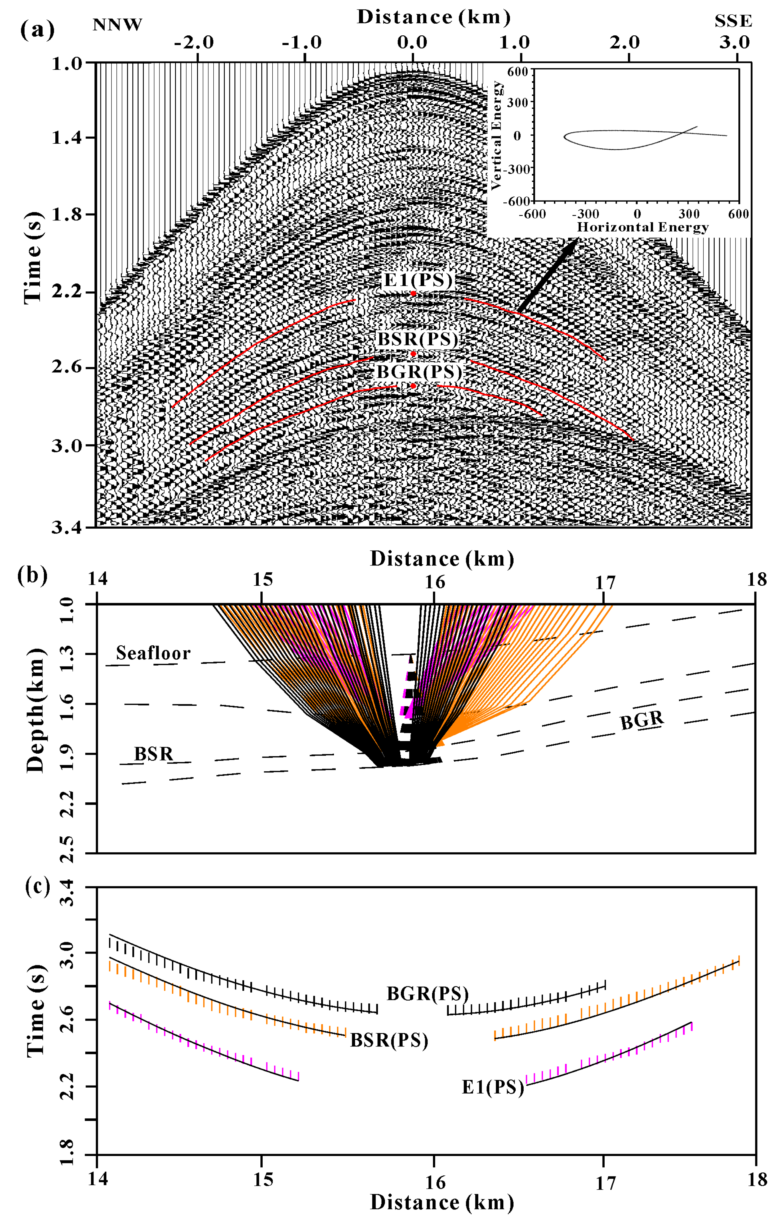
S-wave velocities were determined by trial and error forward modeling of the travel times of converted S-waves from the inline component of OBS data. Here, only the PS-wave type was considered. A part of the P-wave energy converts to S-wave energy at a reflector when the energy does not impinge perpendicularly to the reflecting surface, and then propagates back upwards as an S-wave to the receiver. The interface depths and P-wave velocities obtained as described in the previous section were held constant, and the S-wave velocities were modeled by inverting for Poisson’s ratio in each layer to have the best fit between the observed and calculated PS travel times. This required the correlation of PS arrivals from the inline component with their equivalent P arrivals from the hydrophone component. Because of the possible ambiguity in this correlation, all the PS events with good signal-to-noise ratio were tested for each layer in order to obtain the event with the optimal fit between calculated and observed travel times. A similar method to estimate S-wave velocities from OBS data has been described in several other studies (e.g., References [43,44,45,46]). This procedure was performed on both OBS stations. Figure 5 shows the picking of PS-wave arrivals from the inline component of OBS 7. The inset shows a plot with particle motion and indicates that the energy is mainly horizontal. The two events at about 2.6 s and 2.8 s at minimum offset were identified as PS arrivals corresponding to the BSR and BGR, respectively. A good fit between calculated and observed PS arrivals was obtained, as shown in Figure 5b,c.
2.2.3. Uncertainty of the Velocity Model
There are two primary sources of errors in the final velocity model: projection and travel time inversion. The former is caused by the drift of the OBS from the MCS line during the placement (see Section 2.1). The error in P- and S-wave velocity caused by the geometry projection was evaluated by observing the residual between the calculated and observed travel time picked at near offset of the OBS data, using the final velocity model. The percentage error is defined as the ratio between travel time residual and observed travel time. In order to estimate the uncertainties of travel time inversion, we performed a sensitivity analysis based on the approach as described in the literature [18]: we perturbed the velocity values of each layer until the RMS travel time residual and normalized χ2 increased significantly from the values obtained from the final model. The uncertainties in S-wave velocity from travel time inversion were obtained through perturbing the Poisson’s ratio, following the similar approach as used for the P-wave velocity. We observed that, as expected, the shallow layers are more sensitive to the variation of Poisson’s ratio than the deep layers. In particular, the error in Poisson’s ratio in the layer just above and below the BSR is about 0.012 and 0.04, respectively. The estimation of uncertainty in P-wave and S-wave velocities was performed for all the layers including the water column (Layer 1), as shown in Table 1.
2.3. Estimation of Gas Hydrate and Free Gas Concentrations
The final velocity field obtained from travel time inversion can be used to estimate the concentrations of gas hydrate and free gas in the pore space. In this study, we adopted the theoretical model proposed by References [30,47] to quantify the amounts of gas hydrate and free gas by converting the velocity anomalies with respect to the reference velocities at full-water saturation. The theoretical model was successfully validated by the Ocean Drilling Program (ODP) data (i.e., Leg 164 [47] and Leg 146 [29]). Positive velocity anomalies are considered as an indication for the presence of gas hydrates, while negative velocity anomalies are considered as caused by free gas. This theoretical model is based on a modified Biot-Geertsma-Smit theory and has been successfully applied in this same geographical area (e.g., Reference [27]). The theory includes an explicit dependence on differential pressure and depth and considers the effects of grain cementation at high concentrations of gas hydrates on the shear modulus of the sediment matrix by using a percolation model [48]. The method gives the equations of both P- and S-wave velocities as functions of some physical parameters, such as porosity, compressibility, rigidity, density, and frequency dependence. These parameters can be determined from experimental datasets (Hamilton’s curves [49,50]).
In this study area, no direct measurements for gas hydrate or free gas concentrations are available. The physical parameters (porosity, density, compressibility) adopted for evaluating the reference velocities were taken from Hamilton’s dataset for normally compacted terrigenous sediments [49,50]. The Poisson’s ratio obtained from travel time inversion of converted S-waves was used to evaluate the rigidity of the sediments in each layer. Low Poisson’s ratio and low P-wave velocity indicate that free gas is uniformly distributed in the pore space [30]. A quantitative estimate was obtained by altering the concentration parameters in the theoretical model until modeled seismic velocity matched the theoretical velocity. The uncertainty in concentration estimation is mainly assessed in relation to the uncertainty in the seismic velocities, but also the errors in estimating the physical parameters used to calculate the reference velocities. Previous sensitivity tests performed in this area suggested that porosity is the most important parameter in the estimation of gas hydrate and free gas concentrations, as a variation of ±5% in porosity can be translated into a variation of ±20% and ±7% of gas hydrate and free gas concentrations, respectively [26].
3. Results and Discussion
The final P-wave velocity model determined by the travel time inversion of reflections and refractions from OBS data is shown in Figure 6. The model indicates that the BSR is nearly parallel to the seafloor at about 510–650 m depth below seafloor. The P-wave velocity increases gradually from 1.68 to 1.73 km/s at the seafloor to 2.0 to 2.1 km/s at the BSR. This high P-wave velocity layer with a thickness varying between 150 and300 m just above the BSR can be associated with the presence of gas hydrates. The layer below the BSR shows a low P-wave velocity of about 1.4–1.6 km/s that can be related to the presence of free gas. The BGR occurs at a depth varying between 80 and 160 m below the BSR; in the layer just below the BGR, velocity varies between 2.64 and 2.71 km/s estimated from analysis of the critical refractions in OBS data.
A lateral variation is observed along the velocity model. In the shallow layer just below the seafloor, the overall trend of P-wave velocity shows a lateral increase from the SSE to NNW. In the layer just above the BSR, OBS 7 yields higher P-wave velocity compared to OBS 6, which results in the highest velocity of 2.1 km/s occurring in the eastern part, while the lowest velocity equal to 2.0 km/s is present in the western part of section. Velocity also varies in the free gas layer below the BSR. The lowest velocity (1.4 km/s) occurs in the western part where the BSR is stronger. The P-wave velocity field is in general agreement with previous studies in this area [3,27].
Figure 7 shows the vertical profiles of P- and S-wave velocities and Poisson’s ratio at the OBS locations. The S-wave velocity shows a continuous increase with depth and reaches a value of about 825 m/s at the BSR. Beneath the BSR, no significant increase or decrease was found, as the S-wave velocity is almost insensitive to pore fluid saturation. For each OBS, the Poisson’s ratio shows a relatively continuous decrease with a depth down to BSR and a strong decrease in the free gas layer below the BSR. Moreover, the Poisson’s ratio is similar within each layer. In the layer just above the BSR, a value of 0.405 ± 0.012 and 0.409 ± 0.012 was observed at OBS 6 and OBS 7, respectively. In the free gas layer, a Poisson’s ratio equal to 0.25 ± 0.04 and 0.29 ± 0.04 was obtained, respectively. The Poisson’s ratio in the gas hydrate and free gas layer presented here are in good agreement with the values obtained from another OBS station as per the location in Figure 1, in the same area analyzed by Reference [3]. Their results show that the Poisson’s ratio is 0.405 in the hydrate-bearing sediments and 0.25 in the gas-bearing sediments. This implies that the Poisson’s ratio is fairly uniform, and the gas hydrate reservoir does not show significant variations in this study area.
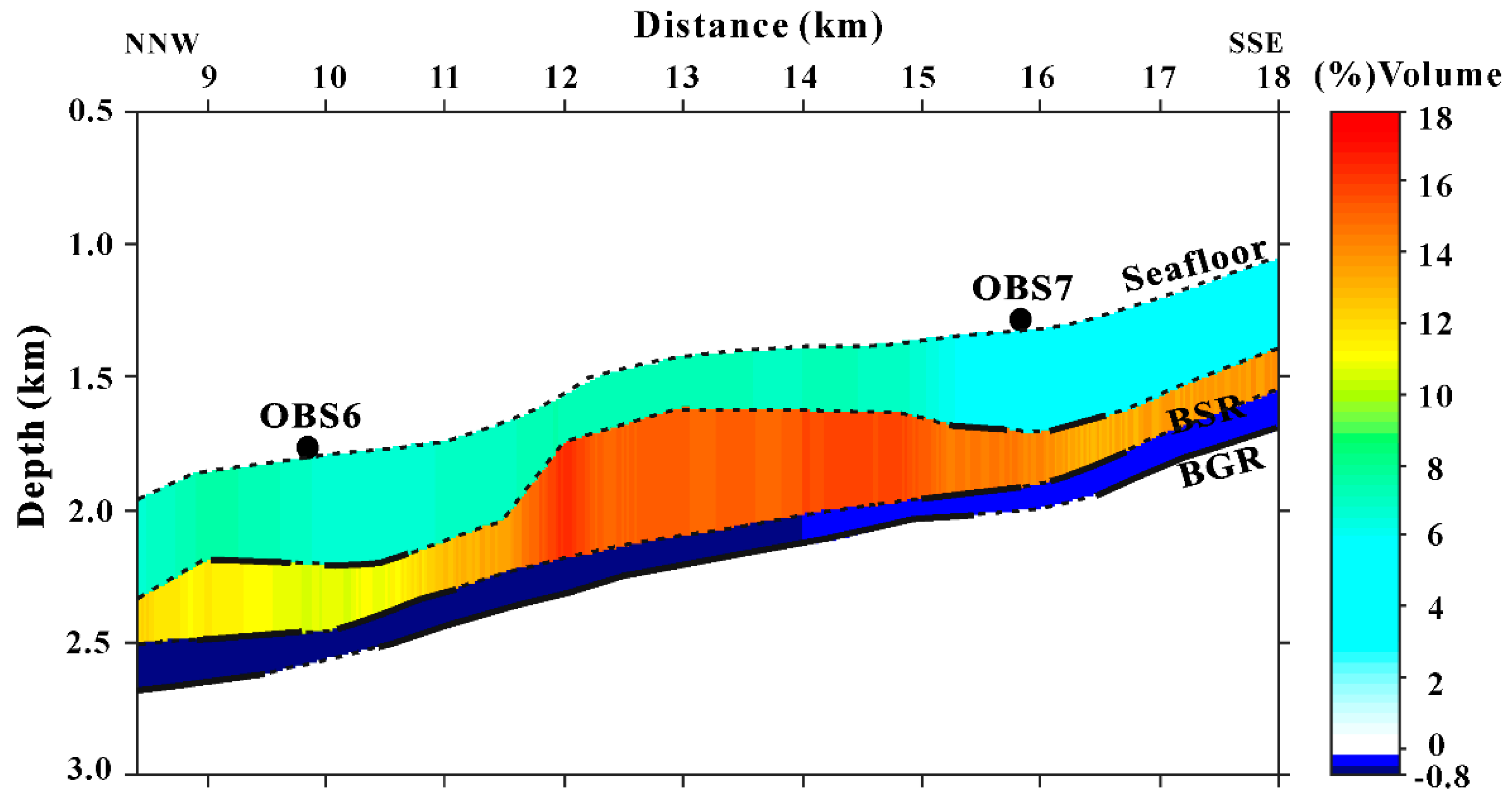
Figure 8 shows the gas hydrate and free gas concentration estimated by comparing the P-wave and S-wave velocity anomalies with the reference velocities. The result indicates that gas hydrate concentration varies from 3% to 7% of total volume in the first layer below the seafloor, while it is in the range of 10% to 15% of total volume in the layer just above the BSR, and free gas concentration is estimated in the range of 0.3% to 0.8% of total volume assuming a uniform distribution in the pore space. Errors related to assumed physical parameters [26] and estimated velocity, as shown in Table 1, correspond to errors in the estimation of gas hydrate and free gas concentrations of about 5% and 0.3% of total volume, respectively. Considering these errors, gas hydrate concentration in the first layer below the seafloor might be close to 0, which means that hydrates probably are not present. Therefore, we suppose that there are water-bearing sediments in the layer just below the seafloor, or, if hydrates are present, the concentration is negligible. This result agrees with previous studies (e.g., References [27,28]). The concentration section does not show any significant lateral variation for gas hydrates or free gas concentrations, respectively. The estimated concentration is comparable with previous studies in this area by other authors. For example, Reference [51] obtained an average concentration of 17.7 and 0.3 percent of volume in the case of gas hydrate and free gas, respectively. If we consider the gas hydrate concentration as a percentage of pore space, it is equal to about 23% to 35% of pore space, which is consistent with the value (23% of pore space) obtained from another OBS analysis by Reference [3] in the same study area. We also compared the estimated hydrate concentrations with the study in the Chilean margin, where the here adopted theoretical model for estimating concentrations was used (e.g., References [52,53,54,55]. The distribution and concentration of gas hydrates along the Chilean margin show strong variation, but comparable concentrations to ours can be observed in some sites [52,54].
The analysis of OBS data has enabled the obtaining of the information of both P- and S-wave velocity fields and it provides new insights into the distribution and quantification of gas hydrate and free gas in marine sediments in the South Shetland margin. The relatively uniform Poisson’s ratio of gas hydrate reservoirs can provide an additional clue for evaluating the rigidity of sediment and thus a reliable concentration when no direct measurements are available. The high concentrations of gas hydrate and free gas suggest that they could be considered as future energy sources. This study can also provide a valuable contribution to the investigation of the relationship between gas hydrate stability and climate change as the polar areas are the most sensitive to global change.
4. Conclusions
The analysis of MCS and OBS data has allowed us to characterize the gas hydrate reservoir in the South Shetland margin. Inversion performed on OBS data provides detailed P- and S-wave velocity information of the subsurface allowing the obtaining of a reliable estimate of gas hydrate and free gas concentrations. The main conclusions of this study are as follows:
- (1)
- We observe a high P-wave velocity layer of 2.0–2.1 km/s just above the BSR, which can be attributed to the presence of gas hydrates. The gas hydrate concentration in this layer is about 10% to 15% of total volume.
- (2)
- We observe a low velocity layer of 1.4–1.6 km/s below the BSR, indicating the presence of free gas. The free gas concentration is about 0.3% to 0.8% of total volume, assuming a uniform distribution of free gas in the pore space.
- (3)
- The Poisson’s ratio obtained by forward modeling of converted S-waves shows good agreement with the previous study performed in this area. This comparison allows us to conclude that the gas hydrate reservoir in this study area shows no significant regional variations from a petrophysical point of view.
Author Contributions
Conceptualization and methodology, U.T., M.G., and G.C.; software, S.S. (Sha Song), S.S. (Sunny Singhroha), and S.B.; supervision, G.C.; investigation, writing—original draft preparation, S.S. (Sha Song); writing—review and editing, U.T., M.G., S.S. (Sunny Singhroha), S.B., and G.C.
Funding
This research was partially supported by the Italian Ministry of Education, Universities and Research (Decreto MIUR No. 631 dd. 8 August 2016) under the extraordinary contribution for Italian participation in activities related to the international infrastructure PRACE—The Partnership for Advanced Computing in Europe (www.prace-ri.eu). Sha Song was supported by the China Scholarship Council grant number 201506400061, and her Short Term Scientific Mission at the CAGE—Centre for Arctic Gas Hydrate, Environment and Climate, Department of Geosciences, UiT The Arctic University of Norway was supported by the Management Committee of the COST-MIGRATE Action (reference code ES1405-050317-082155). Sunny Singhroha and Stefan Bünz were supported by the Research Council of Norway through its Centres of Excellence funding scheme grant No. 223259.
Acknowledgments
The geophysical data were acquired in the frame of the project “Gas Hydrates: impact on climate environmental of the sub-Antarctic regions (BSR)” supported by the Italian National Antarctic Program (PNRA). Sunny Singhroha and Stefan Bünz were supported by the Research Council of Norway through its Centres of Excellence funding scheme, project number 223259/F5.
Conflicts of Interest
The authors declare no conflict of interest.
References
- Sloan, E.D. Clathrate Hydrates of Natural Gases, 2nd ed.; Marcel Dekker, Inc.: New York, NY, USA, 1998; pp. 1–641. ISBN 0824799372. [Google Scholar]
- Kvenvolden, K.A. Gas hydrates-geological perspective and global change. Rev. Geophys. 1993, 31, 173–187. [Google Scholar] [CrossRef]
- Tinivella, U.; Accaino, F. Compressional velocity structure and Poisson’s ratio in marine sediments with gas hydrate and free gas by inversion of reflected and refracted seismic data (South Shetland Islands, Antarctica). Mar. Geol. 2000, 164, 13–27. [Google Scholar] [CrossRef]
- Boswell, R.; Collett, T.S. Current perspectives on gas hydrate resources. Energy Environ. Sci. 2011, 4, 1206–1215. [Google Scholar] [CrossRef]
- Johnson, A. Global resource potential of gas hydrate—A new calculation. Fire Ice Dep. Energy Nat. Energy Technol. Lab. Newsl. 2011, 11, 1–4. [Google Scholar]
- Collett, T.S.; Boswell, R. Resource and hazard implications of gas hydrates in the Northern Gulf of Mexico: Results of the 2009 Joint Industry Project Leg II Drilling Expedition. Mar. Petrol. Geol. 2012, 34, 1–3. [Google Scholar] [CrossRef]
- Yelisetti, S.; Spence, G.D.; Riedel, M. Role of gas hydrates in slope failure on frontal ridge of northern Cascadia margin. Geophys. J. Int. 2014, 199, 441–458. [Google Scholar] [CrossRef]
- Li, A.; Davies, R.J.; Yang, J. Gas trapped below hydrate as a primer for submarine slope failures. Mar. Geol. 2016, 380, 264–271. [Google Scholar] [CrossRef]
- Kvenvolden, K.A. Potential effects of gas hydrate on human welfare. Proc. Natl. Acad. Sci. USA 1999, 96, 3420–3426. [Google Scholar] [CrossRef] [PubMed] [Green Version]
- Kvenvolden, K.A. A primer on the geological occurrence of gas hydrate. In Gas Hydrates: Relevance to World Margin Stability and Climate Change; Henniet, J.P., Mienert, J., Eds.; Geological Society: London, UK, 1998; Volume 137, pp. 9–30. [Google Scholar] [CrossRef]
- Kennett, J.P.; Cannariato, K.G.; Hendy, I.L.; Behl, R.J. Methane Hydrates in Quaternary Climate Change: The Clathrate Gun Hypothesis. In Methane Hydrates in Quaternary Climate Change: The Clathrate Gun Hypothesis; American Geophysical Union: Washington, DC, USA, 2003; Volume 54, pp. 1–217. ISBN 9781118665138. [Google Scholar]
- Bünz, S.; Mienert, J.; Vanneste, M.; Andreassen, K. Gas hydrates at the Storegga Slide: Constraints from an analysis of multi-component, wide-angle seismic data. Geophysics 2005, 70, B19–B34. [Google Scholar] [CrossRef]
- Mienert, J.; Vanneste, M.; Bünz, S.; Andreassen, K.; Haflidason, H.; Sejrup, H.P. Ocean warming and gas hydrate stability on the mid-Norwegian margin at the Storegga Slide. Mar. Pet. Geol. 2005, 22, 233–244. [Google Scholar] [CrossRef]
- Ruppel, C.D. Methane Hydrates and Contemporary Climate Change. Nat. Educ. Knowl. 2011, 3, 29. [Google Scholar]
- Ruppel, C.D.; Kessler, J.D. The interaction of climate change and methane hydrates. Rev. Geophys. 2017, 55, 126–168. [Google Scholar] [CrossRef] [Green Version]
- Hyndman, R.D.; Spence, G.D. A seismic study of methane hydrate marine bottom simulating reflectors. J. Geophys. Res. 1992, 97, 6683–6698. [Google Scholar] [CrossRef]
- Singh, S.C.; Minshull, T.A.; Spence, G.D. Velocity structure of a gas hydrate reflector. Science 1993, 260, 104–207. [Google Scholar] [CrossRef] [PubMed]
- Katzman, R.; Holbrook, W.S.; Paull, C.K. Combined vertical-incidence and wide-angle seismic study of a gas hydrate zone, Blake ridge. J. Geophys. Res. 1994, 99, 17975–17995. [Google Scholar] [CrossRef]
- Korenaga, J.; Holbrook, W.S.; Singh, S.C.; Minshull, T.A. Natural gas hydrates on the southeast US margin: Constraints from full waveform and travel time inversions of wide-angle seismic data. J. Geophys. Res. 1997, 102, 15345–15365. [Google Scholar] [CrossRef]
- Kumar, D.; Sen, M.K.; Bangs, N.L. Gas hydrate concentration and characteristics within Hydrate Ridge inferred from multicomponent seismic reflection data. J. Geophys. Res. 2007, 112. [Google Scholar] [CrossRef]
- Helgerud, M.; Dvorkin, J.; Nur, A.; Sakai, A.; Collett, T. Elastic-wave velocity in marine sediments with gas hydrates: Effective medium modeling. Geophys. Res. Lett. 1999, 26, 2021–2024. [Google Scholar] [CrossRef] [Green Version]
- Chand, S.; Minshull, T.A.; Gei, D.; Carcione, J. Elastic velocity models for gas-hydrate-bearing sediments—A comparison. Geophys. J. Int. 2004, 159, 573–590. [Google Scholar] [CrossRef]
- Dash, R.; Spence, G.D. P-wave and S-wave velocity structure of northern Cascadia margin gas hydrates. Geophys. J. Int. 2011, 187, 1363–1377. [Google Scholar] [CrossRef] [Green Version]
- Andreassen, K.; Berteussen, K.A.; Sognnes, H.; Henneberg, K.; Langhammer, J.; Mienert, J. Multicomponent ocean bottom cable data in gas hydrate investigation offshore of Norway. J. Geophys. Res. 2003, 108, 2399. [Google Scholar] [CrossRef]
- Petersen, C.J.; Papenberg, C.; Klaeschen, D. Local seismic quantification of gas hydrates and BSR characterization from multi-frequency OBS data at northern Hydrate Ridge. Earth Planet Sci. Lett. 2007, 255, 414–431. [Google Scholar] [CrossRef]
- Tinivella, U.; Accaino, F.; Camerlenghi, A. Gas hydrate and free gas distribution form inversion of seismic data on the South Shetland margin (Antarctica). Mar. Geophys. Res. 2002, 23, 109–123. [Google Scholar] [CrossRef]
- Loreto, M.F.; Tinivella, U.; Accaino, F.; Giustiniani, M. Gas hydrate reservoir characterization by geophysical data analysis (offshore Antarctic Peninsula). Energies 2011, 4, 39–56. [Google Scholar] [CrossRef]
- Loreto, M.F.; Tinivella, U. Gas hydrate versus geological features: The South Shetland case study. Mar. Pet. Geol. 2012, 36, 164–171. [Google Scholar] [CrossRef]
- Tinivella, U.; Carcione, J.M. Estimation of gas-hydrate concentration and free-gas saturation from log and seismic data. Lead. Edge 2001, 20, 200–203. [Google Scholar] [CrossRef]
- Tinivella, U. The seismic response to overpressure versus gas hydrate and free gas concentration. J. Seism. Explor. 2002, 11, 283–305. [Google Scholar]
- Tinivella, U.; Accaino, F.; Della Vedova, B. Gas hydrates and active mud volcanism on the South Shetland continental margin, Antarctic Peninsula. Geo-Mar. Lett. 2008, 28, 97–106. [Google Scholar] [CrossRef]
- Maldonado, A.; Larter, R.D.; Aldaya, F. Forearc tectonic evolution of the South Shetland Margin, Antarctic Peninsula. Tectonics 1994, 13, 1345–1370. [Google Scholar] [CrossRef]
- Kim, Y.; Kim, H.S.; Larter, R.D.; Camerlenghi, A.; Gambôa, L.A.P.; Rudowski, S. Tectonic deformation in the upper crust and sediments at the South Shetland Trench. In Geology and Seismic Stratigraphy of the Atlantic Margin; Cooper, A.K., Barker, P.T., Brancolini, G., Eds.; American Geophysical Union: Washington, DC, USA, 1995; Volume 68, pp. 157–166. ISBN 9781118669013. [Google Scholar]
- Pankhurst, R.J. The Paleozoic and Andean magmatic arcs of West Antarctica and southern South America. In Plutonism from Antarctica to Alaska; Kay, S.M., Rapela, C.W., Eds.; Geological Society of Amer: Boulder, CO, USA, 1990; Volume 241, pp. 1–7. ISBN 9780813722412. [Google Scholar]
- Larter, R.D.; Barker, P.F. Effects of ridge crest-trench interaction on Antarctic-Phoenix spreading: Forces on a young subducting plate. J. Geophys. Res. 1991, 96, 19583–19607. [Google Scholar] [CrossRef]
- Jin, Y.K.; Larter, R.D.; Kim, Y.; Nam, S.H.; Kim, K.J. Post-subduction margin structures along Boyd Strait, Antarctic Peninsula. Tectonophysics 2002, 346, 187–200. [Google Scholar] [CrossRef]
- Dietrich, R.; Rülke, A.; Ihde, J.; Lindner, K.; Miller, H.; Niemeier, W.; Schenke, H.W.; Seeber, G. Plate kinematics and deformation status of the Antarctic Peninsula based on GPS. Glob. Planet. Chang. 2004, 42, 313–321. [Google Scholar] [CrossRef]
- Marín-Moreno, H.; Giustiniani, M.; Tinivella, U.; Pinero, E. The challenges of quantifying the carbon stored in Arctic marine gas hydrate. Mar. Pet. Geol. 2016, 71, 76–82. [Google Scholar] [CrossRef] [Green Version]
- Cohen, J.K.; Stockwell, J.W. CWP/SU: Seismic Unix Release 4.0: A free Package for Seismic Research and Processing; Center for Wave Phenomena, Colorado School of Mines: Golden, CO, USA, 2008; pp. 1–153. [Google Scholar]
- Gaiser, J.E. Applications for vector coordinate systems of 3-D converted wave data. Lead. Edge 1999, 18, 1290–1300. [Google Scholar] [CrossRef]
- Zelt, C.A.; Smith, R.B. Seismic travel time inversion for 2-D crustal velocity structure. Geophys. J. Int. 1992, 108, 16–34. [Google Scholar] [CrossRef]
- Yelisetti, S. Seismic structure, gas hydrate, and slumping studies on the Northern Cascadia margin using multiple migration and full waveform inversion of OBS and MCS data. Ph.D. Thesis, University of Victoria, Victoria, BC, Canada, 2014. [Google Scholar]
- Westbrook, G.K.; Chand, S.; Rossi, G.; Long, S.; Bünz, S.; Camerlenghi, A.; Carcione, J.M.; Dean, S.; Foucher, J.P.; Flueh, E.; et al. Estimation of gas-hydrate concentration from multi-component seismic data at sites on the continental margins of NW Svalbard and the Storegga region of Norway. Mar. Pet. Geol. 2008, 25, 744–758. [Google Scholar] [CrossRef]
- Peacock, S.; Westbrook, G.K.; Bais, G. S-wave velocities and anisotropy in sediments entering the Nankai subduction zone, offshore Japan. Geophys. J. Int. 2010, 180, 743–758. [Google Scholar] [CrossRef]
- Exley, R.J.K.; Westbrook, G.K.; Haacke, R.R.; Peacock, S. Detection of Seismic anisotropy using ocean bottom seismometers: A case study from northern headwall of Storegga Slide. Geophys. J. Int. 2010, 183, 188–210. [Google Scholar] [CrossRef]
- Satyavani, N.; Sain, K.; Gupta, H.K. Ocean bottom seismometer data modeling to infer gas hydrate saturation in Krishna-Godavari (KG) basin. J. Nat. Gas Sci. Eng. 2016, 33, 908–917. [Google Scholar] [CrossRef]
- Tinivella, U. A method for estimating gas hydrate and free gas concentrations in marine sediments. Boll. Geofis. Teor. Appl. 1999, 40, 19–30. [Google Scholar]
- Leclaire, P. Propagation Acoustique dans les Milieux Poreux Soumis au Gel-Modélisation et Expérience. Ph.D. Thesis, Université Paris, Paris, France, 1992. [Google Scholar]
- Hamilton, E.L. Variations of density and porosity with depth in deep-sea sediments. J. Sediment. Res. 1976, 46, 280–300. [Google Scholar]
- Hamilton, E.L. Vp/Vs and Poisson’s ratios in marine sediments and rocks. J. Acoust. Soc. Am. 1979, 66, 1093–1101. [Google Scholar] [CrossRef]
- Tinivella, U.; Loreto, M.F.; Accaino, F. Regional versus detailed velocity analysis to quantify hydrate and free gas in marine sediments: The south Shetland margin target study. Geol. Soc. Spec. Publ. 2009, 319, 103–119. [Google Scholar] [CrossRef]
- Vargas-Cordero, I.; Tinivella, U.; Villar-Muñoz, L.P.; Bento, J. High Gas Hydrate and Free Gas Concentrations: An Explanation for Seeps Offshore South Mocha Island. Energies 2018, 11, 3062. [Google Scholar] [CrossRef]
- Villar-Muñoz, L.; Bento, J.P.; Klaeschen, D.; Tinivella, U.; Vargas-Cordero, I.; Behrmann, J.H. A first estimation of gas hydrates offshore Patagonia (Chile). Mar. Pet. Geol. 2018, 96, 232–239. [Google Scholar] [CrossRef]
- Vargas-Cordero, I.; Tinivella, U.; Villar-Muñoz, L. Gas Hydrate and Free Gas Concentrations in Two Sites inside the Chilean Margin (Itata and Valdivia Offshores). Energies 2017, 10, 2154. [Google Scholar] [CrossRef]
- Vargas-Cordero, I.; Tinivella, U.; Accaino, F.; Loreto, M.F.; Fanucci, F. Thermal state and concentration of gas hydrate and free gas of Coyhaique, Chilean Margin (44°30′ S). Mar. Pet. Geol. 2010, 27, 1148–1156. [Google Scholar] [CrossRef]
Figure 1.
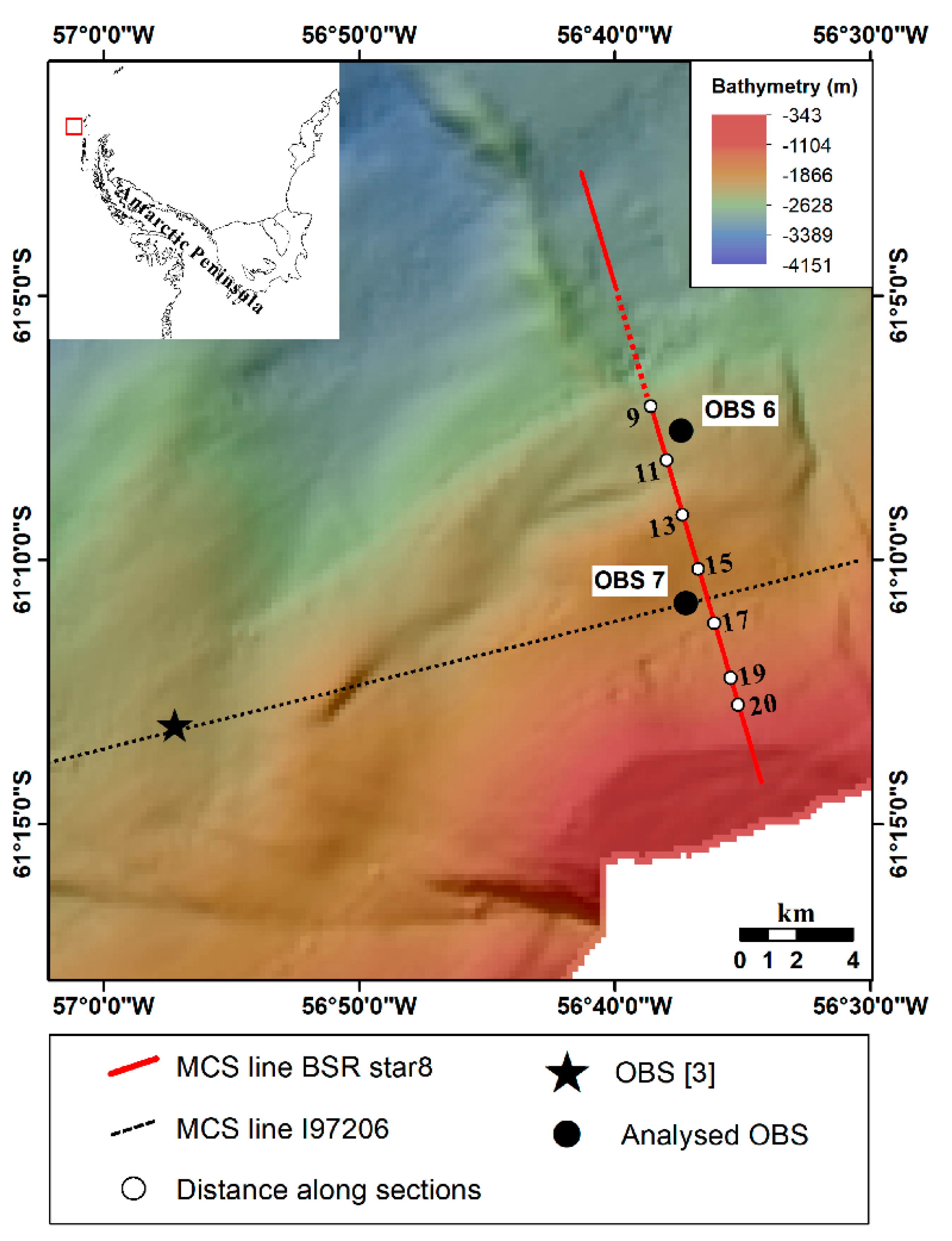
Bathymetric map of the study area (modified after References [27,28]), indicating the locations of seismic lines and ocean bottom seismometers (OBSs). The black circles indicate the positions of OBSs. The red line indicates the multi-channel seismic (MCS) line shown in Figure 2; the red dotted line indicates the gap for the MCS line; the white circles and numbers show the corresponding distances along sections. The star and dashed line mark the OBS and seismic line analyzed in the study by Reference [3].
Figure 1.
Bathymetric map of the study area (modified after References [27,28]), indicating the locations of seismic lines and ocean bottom seismometers (OBSs). The black circles indicate the positions of OBSs. The red line indicates the multi-channel seismic (MCS) line shown in Figure 2; the red dotted line indicates the gap for the MCS line; the white circles and numbers show the corresponding distances along sections. The star and dashed line mark the OBS and seismic line analyzed in the study by Reference [3].

Figure 2.
(a) Time migrated section of part of MCS line BSRstar8. An automatic gain control (AGC) with a time window of 400 ms was applied to better image the bottom simulating reflection (BSR). The solid circles indicate the OBS locations projected on the MCS line. The boxes indicate the portion of the seismic line shown in panels (b) and (c); panels (b) and (c) report the correlation between the hydrophone component of OBS 7 and the MCS seismic section. Note that the two datasets have a different time axis due to the spatial drift of the OBS from the MCS line during the sinking. The travel time picks of P-wave reflections (Seafloor, E1, BSR) on the hydrophone data are shown as red lines on the OBS panels. See text for details; panel (d) close-up view of OBS panel (c) showing the BSR. TWT: two-way time.

Figure 3.
Hydrophone component of OBS 7 showing travel time picks (red lines) of refraction. The signal above the refraction is noise. The horizontal axis is the distance between projected OBS position and shot position. The time is reduced with a velocity of 3.2 km/s.
Figure 3.
Hydrophone component of OBS 7 showing travel time picks (red lines) of refraction. The signal above the refraction is noise. The horizontal axis is the distance between projected OBS position and shot position. The time is reduced with a velocity of 3.2 km/s.

Figure 4.
(a) Hydrophone component of OBS 7 showing travel time picks (red lines) of P-wave reflections used in the inversion. The horizontal axis is the distance between projected OBS position and shot position. The travel times at minimum offset corresponding to the reflections (Seafloor, E1, BSR) are indicated with the red dots; (b) P-wave ray diagram modeled on OBS 7. For clarity, rays modeled on MCS data are not shown; (c) the fit between calculated (solid lines) and observed (short vertical lines) travel times for OBS 7; (d) the fit between calculated (solid lines) and observed (short vertical lines) travel times for MCS data. For better visibility, every sixth shot is shown. The MCS time is reduced with a velocity of 4 km/s. The colors of observed travel times are the same as those of corresponding rays in panel (b). BGR: base of the free gas layer.
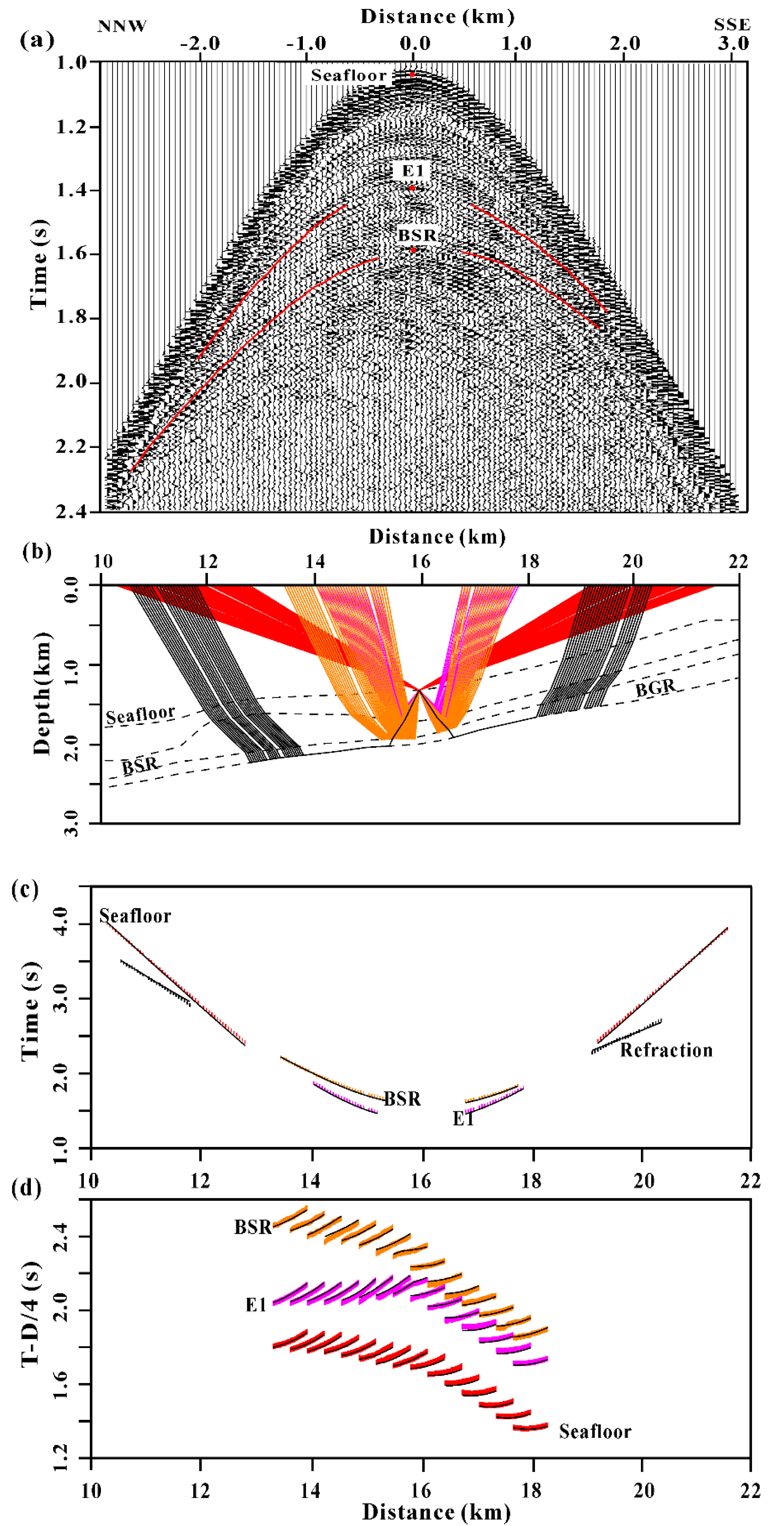
Figure 5.
(a) Inline component of OBS 7 showing travel time picks (red lines) of PS-waves. The horizontal axis is the distance between projected OBS position and shot position. The travel times at minimum offset corresponding to the PS-waves are indicated with the red dots. The inset shows the particle motion plot for the E1 (PS) event; (b) PS-wave ray diagram modeled on OBS 7; (c) the fit between calculated (solid lines) and observed (short vertical lines) travel times. The colors of observed travel times are the same as those of corresponding rays in panel (b).

Figure 6.
P-wave velocity model determined by inversion of MCS and OBS data. Solid boundary lines indicate the P-wave ray coverage for the different layer interfaces. The grey shading indicates the area with no ray coverage.
Figure 6.
P-wave velocity model determined by inversion of MCS and OBS data. Solid boundary lines indicate the P-wave ray coverage for the different layer interfaces. The grey shading indicates the area with no ray coverage.

Figure 7.
The seismic velocity profiles (red lines) after inversion and reference velocity curves (black dotted lines) and Poisson’s ratio profiles extracted at the locations of OBS 6 (a) and OBS 7 (b). Depth is measured below the seafloor (bsf).
Figure 7.
The seismic velocity profiles (red lines) after inversion and reference velocity curves (black dotted lines) and Poisson’s ratio profiles extracted at the locations of OBS 6 (a) and OBS 7 (b). Depth is measured below the seafloor (bsf).
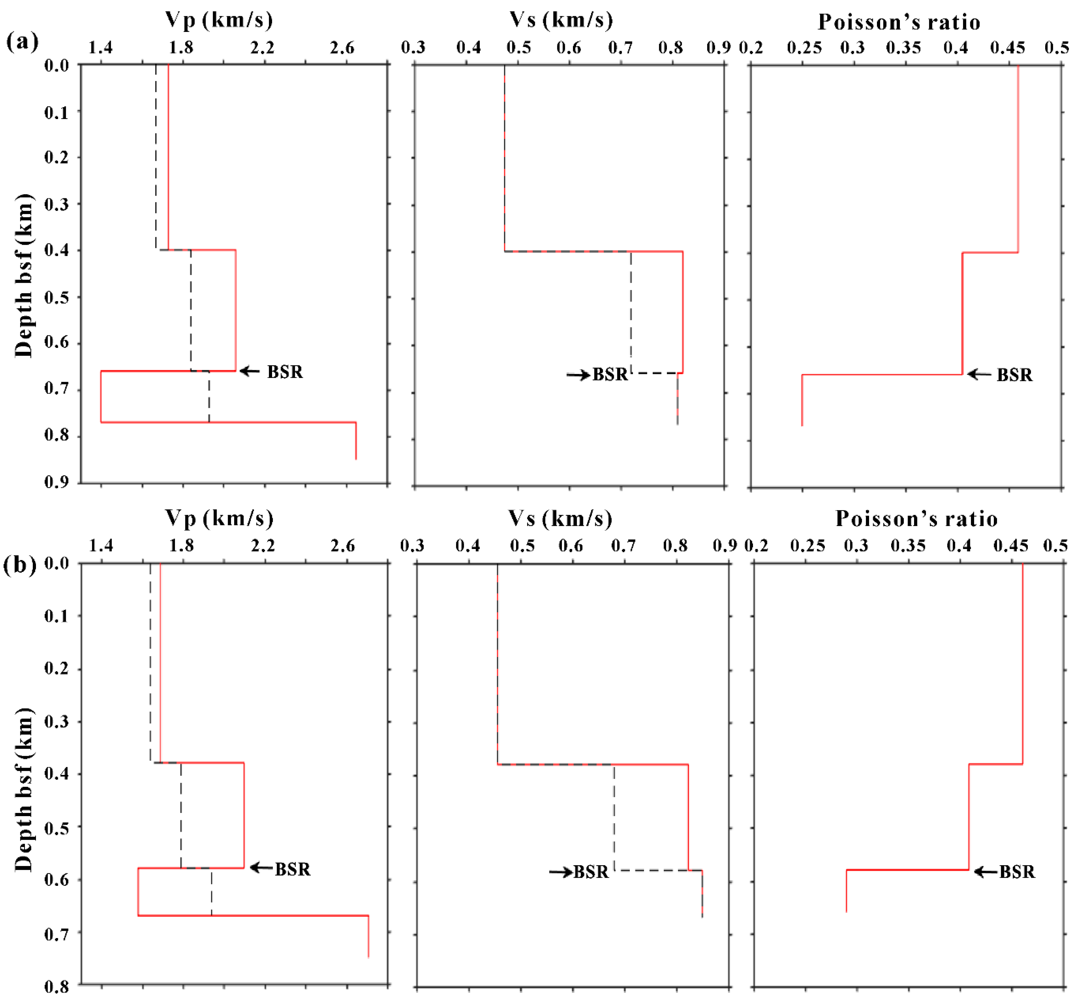
Figure 8.
Concentration section of gas hydrate (positive values) and free gas (negative values).


Table 1.
Percentage errors of P-wave and S-wave velocities estimated from the sensitivity analysis.
| Layer | Error in P-Wave Velocity | Error in S-Wave Velocity | ||||
|---|---|---|---|---|---|---|
| Projection Error (%) | Inversion Error (%) | Final Error (%) | Projection Error (%) | Inversion Error (%) | Final Error (%) | |
| 1 | NO | 1 | 1 | NO | NO | NO |
| 2 | 2 | 5 | 7 | 2 | 4 | 6 |
| 3 | 1 | 7 | 8 | 1 | 7 | 8 |
| 4 | 1 | 7 | 8 | 1 | 9 | 10 |
© 2018 by the authors. Licensee MDPI, Basel, Switzerland. This article is an open access article distributed under the terms and conditions of the Creative Commons Attribution (CC BY) license (http://creativecommons.org/licenses/by/4.0/).
Share and Cite
MDPI and ACS Style
Song, S.; Tinivella, U.; Giustiniani, M.; Singhroha, S.; Bünz, S.; Cassiani, G. OBS Data Analysis to Quantify Gas Hydrate and Free Gas in the South Shetland Margin (Antarctica). Energies 2018, 11, 3290. https://doi.org/10.3390/en11123290
AMA Style
Song S, Tinivella U, Giustiniani M, Singhroha S, Bünz S, Cassiani G. OBS Data Analysis to Quantify Gas Hydrate and Free Gas in the South Shetland Margin (Antarctica). Energies. 2018; 11(12):3290. https://doi.org/10.3390/en11123290
Chicago/Turabian StyleSong, Sha, Umberta Tinivella, Michela Giustiniani, Sunny Singhroha, Stefan Bünz, and Giorgio Cassiani. 2018. "OBS Data Analysis to Quantify Gas Hydrate and Free Gas in the South Shetland Margin (Antarctica)" Energies 11, no. 12: 3290. https://doi.org/10.3390/en11123290
Note that from the first issue of 2016, this journal uses article numbers instead of page numbers. See further details here.