Estimation of the Time-Varying High-Intensity Heat Flux for a Two-Layer Hollow Cylinder

Abstract

Gun barrels are subjected to time-varying high-intensity heat flux under multiple firing, which may damage the material and limit the overall performance of the gun. In order to monitor the thermal state of a gun barrel, an inverse method coupling the finite difference method with the sequential function specification method was developed to estimate the unknown time-varying heat flux imposed on the inner wall of a gun barrel. A two-layer hollow cylindrical tube was assumed with the convection heat transfer boundary condition on the outer wall of the tube. A direct heat transfer model was developed, and was used to estimate the temporal distribution of boundary heat flux in approximately real time based on the measured transient temperature at some positions on the outer wall of the gun barrel. Numerical tests were performed to verify the effectiveness and reliability of this method by investigating the influence of temperature measurement noises and future time step selection. The results show that the proposed method has high precision and efficiency in extracting the time-varying heat flux under one-shot and three-shot firing conditions. When there is a measurement noise, this method has good anti-illness characteristics and can achieve better results by appropriately selecting the value of a future time step.

1. Introduction

In engineering, some thermal equipment with a hollow-cylindrical shape experiences extremely severe thermal shock. Corrosion effects and thermal stress induced by transient high-intensity heat flux may damage the material and limit the overall performance of a thermal system. For example, in cylindrical gun barrels, the high temperature occurring at the commencement of rifling is the primary cause of gun barrel erosion. The large heat input from multiple firing can cause damage to the gun material, especially the very thin chrome layer that coats on the inner wall of the gun barrel, e.g., melting, cracking, erosion, and wear. An excellent review of gun barrel erosion is given by Sopok et al. [1,2]. Furthermore, a large temperature gradient may exist between the inner and outer walls of the gun barrel, generating great thermal stress [3,4], which may cause damage to the gun material. Therefore, better understanding of the thermal loads acting on gun barrels is vital for their application.

Some studies have focused on the heat transfer of gun barrels under firing. For example, Değirmenci et al. [3] employed a thermo-mechanical model using finite element code generated by ABAQUS software to investigate the effect of grain size and initial temperatures of double base propellants on internal pressure, bullet velocity, and barrel heat transfer, which was validated with experimental data. This research found that the barrel experienced high thermal stresses during successive shootings. Additionally, Şentürk et al. [4] conducted 3D transient heat transfer and thermal stress analysis of a 7.62 mm gun barrel using experimental, numerical, and analytical methods with a thermo-mechanical approach. The commercial ANSYS software was employed to obtain the temperature distribution in the radial and axial directions of the barrel. Their test results imply that the temperature rise in the gun barrel is one of the most important design criteria that must be accounted for. Furthermore, Sun et al. [5] have studied the transient temperature response of a hollow cylinder subjected to periodic boundary conditions and investigated the effects of different parameters on the maximum temperature of the inner surface. Mishra et al. [6] proposed a new scheme for computing gun barrel temperature variation with time by coupling the internal ballistics code and finite element model. In their study, heat flux to the gun bore surface was determined from the computed results of internal ballistics code (GUMTEMP8.EXE) and is approximated as an exponentially decaying form. The simulation results were found to match satisfactorily to the corresponding experimental measurements.

Moreover, some scholars have estimated the thermal state of gun barrel by establishing inverse heat transfer problem (IHTP). For instance, Chen et al. [7], Lee et al. [8], and Noh et al. [9,10,11,12] applied an input-estimation method, conjugate gradient method, and Kalman filter, coupled with the recursive least-squares algorithm to perform thermal analysis in order to estimate the unknown boundary condition. In recent years, Noh et al. [11] proposes a three-dimensional inverse heat transfer analysis model for estimating the heat flux in real gun barrels with varying cross-sections. Besides, Noh et al. [12] investigated the effects of a hollow cylindrical tube’s thickness and material properties on estimated time delay and waveform distortion in a one-dimensional inverse heat transfer analysis model for gun barrel. Jablonski et al. [13] proposed an inverse model to estimate the total heat flux applied to the bore surface as well as the transient history. A parametric study was conducted to determine the influence of a sensor time-constant, sensor location within the gun barrel, and measurement bias on the accuracy of the estimated heat flux, as applied to a 155mm gun barrel. For a thermal system, it is important to identify the boundary heat flux variation for temperature calculation [14,15].

Inverse heat transfer problem (IHTP) uses limited measurable temperature information as input to estimate the unknown temperature, heat flux, heat source, geometry, or thermal properties of a heat transfer system. IHTP has been applied widely in engineering [16,17,18,19,20,21,22,23,24], however, it is difficult to solve because it is a classical ill-posed problem, which indicates any small disturbances in the input data may result in large fluctuations and errors in the estimated results. Many valuable methods have been developed for the solution of IHTP [9,17,19,24,25,26,27]. According to the computational process, these methods can be classified as whole domain (iterative) and sequential (non-iterative) methods [28]. Sequential algorithms have the advantage of being highly efficient, as compared to whole domain methods, without a significant loss of accuracy. The sequential function specification method (SFSM) is an important sequential method introduced by Beck (1985) [25], which is widely used in literature for estimating heat flux in different applications [29,30,31,32,33,34]; however, no research has been found regarding its application in the gun thermal problem.

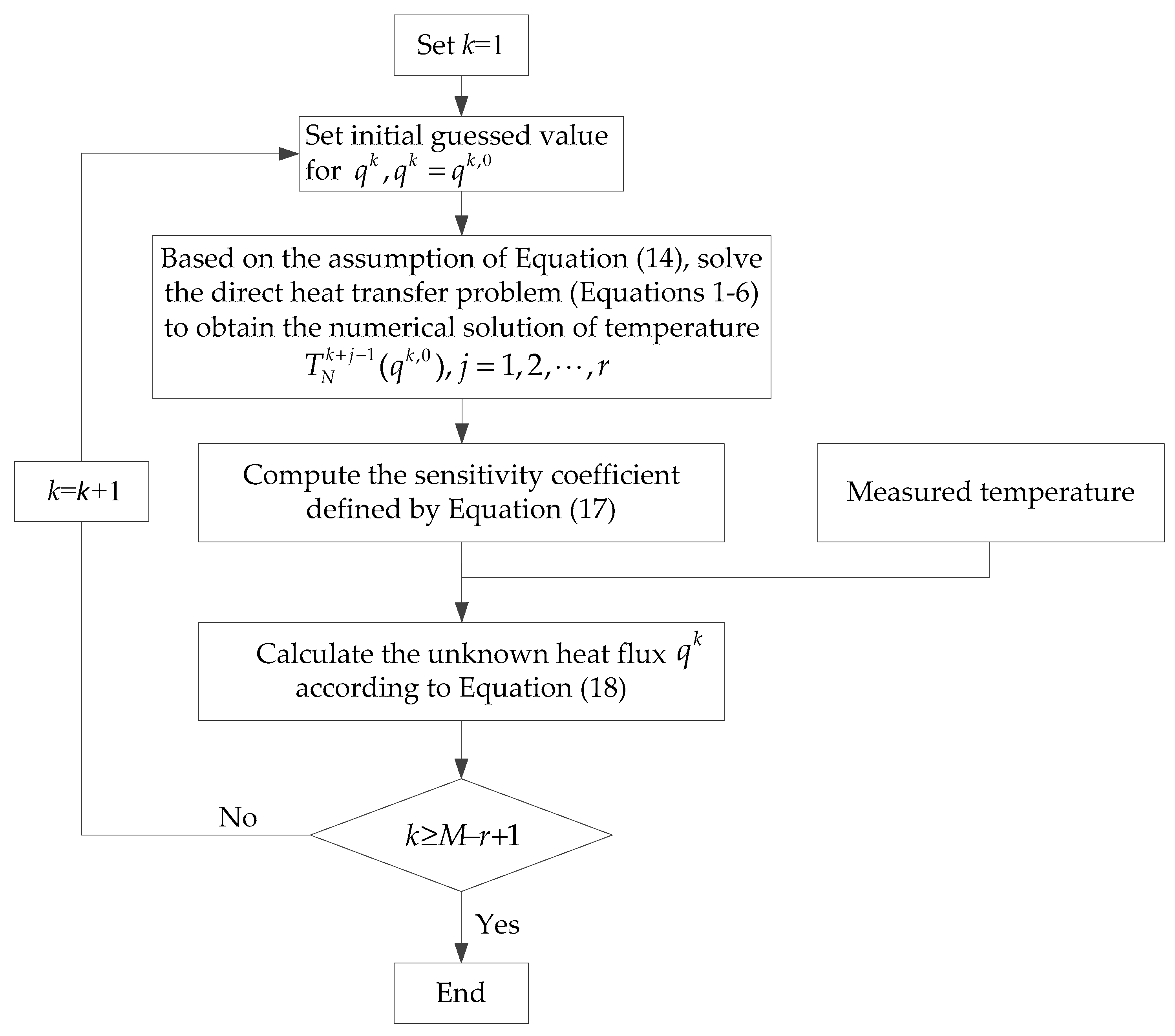
The goal of this study is to develop a method to determine the boundary heat flux condition of a gun’s inner wall under firing. Firstly, a mathematical model for a two-layer gun barrel thermal system is established, followed by a numerical solution. Then, an inverse heat transfer problem is solved by incorporating the mathematical model with a sequential function specification method to determine the unknown boundary heat flux. A series of numerical tests are conducted to verify the feasibility and identify the limitations of the proposed method, including the effects of temperature measurement noises and the parameter of future time step. Finally, this method is applied to the continuously firing process to obtain the periodically time-varying inner boundary condition of the gun barrel.

2. Direct Heat Transfer Model of a Two-Layer Gun Barrel

The gun barrel is modeled as a two-layer hollow tube. The cross-section of the barrel’s geometry in the axial direction is shown in Figure 1a. When firing, the inner wall receives heat flux q(t) from high-temperature combustion gas and bullet friction. The outer wall is assumed to undergo convective heat transfer with the environment. The main material of the barrel is stainless steel (outer layer), and the inner wall is coated by a very thin layer of chromium. The radius of the inner wall, the interface between the chromium and stainless steel, and the outer wall are defined as R_in, R_mid, and R_out, respectively. For more efficient calculation, the following assumptions are made [35]: (1) The material’s thermal properties are constant; (2) the contact thermal resistance at the interface between the inner and outer layers can be neglected; (3) the heat flux on the inner wall is regarded as the comprehensive result of combustion gas and bullet friction; and (4) the heat flux distribution is uniform along circumferential and axial directions. Based on the above assumptions, the heat transfer model of the two-layer gun barrel is simplified to be a one-dimensional transient heat transfer problem, as shown in Figure 1b.

In the cylindrical coordinate system, the governing equations, initial condition, and boundary conditions of a two-layer gun barrel thermal system are given as follows [8]:

$$\frac{{\rho }_1{C}_1}{{\lambda }_1}\frac{\partial T(R,t)}{\partial t}=\frac{{\partial }^{2}T(R,t)}{\partial R^2}+\frac{1}{R}\frac{\partial T(R,t)}{\partial R},R_{\mathrm{in}}<R<R_{\mathrm{mid}},0<t\le t_f$$

(1)

$$-{\lambda }_1\frac{\partial T(R,t)}{\partial R}=q(t),R=R_{\mathrm{in}}$$

(2)

$$-{\lambda }_1\frac{\partial T(R,t)}{\partial R}=-{\lambda }_2\frac{\partial T(R,t)}{\partial R},T|{}_{\mathrm{chrome}}=T|{}_{\mathrm{steel}},R=R_{\mathrm{mid}}$$

(3)

$$\frac{{\rho }_2{C}_2}{{\lambda }_2}\frac{\partial T(R,t)}{\partial t}=\frac{{\partial }^{2}T(R,t)}{\partial R^2}+\frac{1}{R}\frac{\partial T(R,t)}{\partial R},R_{\mathrm{mid}}<R<R_{\mathrm{out}},0<t\le t_f$$

(4)

$$-{\lambda }_2\frac{\partial T(R,t)}{\partial R}=h(T-T_{\infty }),R=R_{\mathrm{out}}$$

(5)

$$T(R,0)=T_0,R_{\mathrm{in}}\le R\le R_{\mathrm{out}}$$

(6)

where T is the gun barrel’s temperature as a function of R and t; R is the radial coordinate and t is the time; ${\rho }_1$, $C_1$ and ${\lambda }_1$ are the density, heat capacity and thermal conductivity of the chrome, respectively; ${\rho }_2$, $C_2$ and ${\lambda }_2$ are the corresponding properties of the stainless steel; $T_{\infty }$ is the ambient temperature; $T_0$ is the initial temperature; h is the heat convection coefficient between the barrel outer wall and the surrounding atmosphere; and $t_f$ is the total time period.

In order to numerically solve the above one-dimensional heat transfer model, the geometry of the gun barrel is meshed into N − 1 equal parts along the radial (R) direction, as shown in Figure 2a. Each node i (i = 2, 3, etc., N − 1) represents a control volume, $V_i$, which is similar to a ring with a peripheral thickness ΔR and a circumferential angle of 360°, as shown in Figure 2b. Node 1 and N are placed on the inner and outer walls, respectively; therefore, the thickness of control volumes $V_1$ and $V_N$ is ΔR/2. Node n is located at the interface between the chrome and steel materials. The time domain ($t_f$) is discretized into M elements. $T_i^k$ represents the temperature of the node i at specific time $t_k$, that is $T_i^k=T(R_i,t_k)$, $R_i=R_{\mathrm{in}}+(i-1)\Delta R$, $t_k=k\Delta \tau$, $i=1,2,\cdots ,N$, and $k=1,2,\cdots ,M$. The spatial and temporal element sizes are defined by:

$$\Delta R=(R_{\mathrm{out}}-R_{\mathrm{in}})/(N-1)$$

(7)

$$\Delta \tau =t_f/M$$

(8)

The direct problem of the heat transfer process defined by Equations (1)–(6) is concerned with the determination of the gun barrel transient temperature field when the geometry, thermal properties, and conditions at all boundaries are known. The heat balance method and tri-diagonal matrix algorithm are applied to obtain the numerical solutions of Equations (1)–(6). The temperature sensor is embedded on the outer wall surface to record the temperature change, denoted by ${(T_N^k)}_{\mathrm{mea}}$.

By applying the law of energy conservation to each control volume $V_i$ (i = 1, 2, etc., N), and taking backward differential for the time derivative term, the discretization equations for all nodes can thus be derived according to the Fourier heat conduction law:

$$C_1{V}_1\frac{T_1^k-T_1^{k-1}}{\Delta \tau }={\lambda }_1\cdot 2\pi \left(R_1+\frac{\Delta R}{2}\right)\frac{T_2^k-T_1^k}{\Delta R}+q^k\cdot 2\pi R_1,i=1$$

(9)

$${\rho }_1{C}_1{V}_i\frac{T_i^k-T_i^{k-1}}{\Delta \tau }={\lambda }_1\cdot 2\pi \left(R_i+\frac{\Delta R}{2}\right)\frac{T_{i+1}^k-T_i^k}{\Delta R}+{\lambda }_1\cdot 2\pi \left(R_i-\frac{\Delta R}{2}\right)\frac{T_{i-1}^k-T_i^k}{\Delta R},i=2,3,\cdots ,n-1$$

(10)

$$-\frac{{\lambda }_1(T_{n-1}^k-T_n^k)}{\Delta R}=-\frac{{\lambda }_2(T_n^k-T_{n+1}^k)}{\Delta R},i=n$$

(11)

$${\rho }_2{C}_2{V}_i\frac{T_i^k-T_i^{k-1}}{\Delta \tau }={\lambda }_2\cdot 2\pi \left(R_i+\frac{\Delta R}{2}\right)\frac{T_{i+1}^k-T_i^k}{\Delta R}+{\lambda }_2\cdot 2\pi \left(R_i-\frac{\Delta R}{2}\right)\frac{T_{i-1}^k-T_i^k}{\Delta R},i=n+1,\cdots ,N-1$$

(12)

$${\rho }_2{C}_2{V}_N\frac{T_N^k-T_N^{k-1}}{\Delta \tau }={\lambda }_2\cdot 2\pi \left(R_N-\frac{\Delta R}{2}\right)\frac{T_{N-1}^k-T_N^k}{\Delta R}+h(T_{\infty }-T_N)\cdot 2\pi R_N,i=N$$

(13)

where

$$V_1=\pi \left[{(R_1+\Delta R/2)}^2-R_1^2\right],V_i=\pi \left[{(R_i+\Delta R/2)}^2-{(R_i-\Delta R/2)}^2\right],V_N=\pi \left[R_N^2-{(R_N-\Delta R/2)}^2\right]$$

The temperature of each node, $T_i^k$, can be obtained by solving Equations (9)–(13), utilizing a tri-diagonal matrix algorithm. In the solution of IHTP, the above direct heat transfer model is continuously called as a subroutine, and thus reasonable simplification can greatly improve the calculation efficiency.

3. Inverse Heat Transfer Problem

In essence, the time-varying heat flux q(t) on the inner wall is regarded as the only unknown in Equations (1)–(6). The present inverse problem is to estimate the unknown boundary heat flux q(t) by utilizing some measured temperature and other known boundary conditions and properties. In our research, the measured temperature is generated by adding Gaussian white noise to the exact calculated temperature with a given boundary heat flux. For the following inverse calculation, the SFSM algorithm is applied to find the unknown heat flux by using the simulated measured temperature.

3.1. Sequential Function Specification Method

The time-varying heat flux function is discretized into a set of components $q^k$ ($k=1,2,\cdots ,M$) according to Section 2. SFSM is applied here to estimate the heat flux components from $q^1$ to $q^M$ sequentially in time. Each component $q^k$ is determined by using the future temperature information within the time period $[t_k,t_{k+r-1}]$, where r is a pre-defined number of future time step. The details for the SFSM algorithm are summarized as follows:

Firstly, for stability, it is temporarily assumed that the heat flux components are equal over “r” future time steps, that is:

$$q^k=q^{k+1}=q^{k+2}=\cdots =q^{k+r-1}$$

(14)

Then, the objective function $J(q_k)$ is to be minimized in order to determine $q^k$, defined as the sum of the squared temperature errors:

$$J(q^k)={\displaystyle \sum _{j=1}^r{\left[{(T_N^{k+j-1})}_{\mathrm{mea}}-T_N^{k+j-1}(q^k)\right]}^2}$$

(15)

where ${(T_N^{k+j-1})}_{\mathrm{mea}}$ and $T_N^{k+j-1}$ are the measured and calculated temperature of the outer wall.

Since the temperature T is a continuous function of heat flux q, the calculated temperature $T_N^{k+j-1}$ can be obtained by using the first-order Taylor expansion [25]:

$$T_N^{k+j-1}(q^k)=T_N^{k+j-1}(q^{k,0})+Z_N^{k,j-1}(q^k-q^{k,0})$$

(16)

where $q^{k,0}$ is an initial guess for the unknown heat flux component $q^k$ and is usually set equal to zero or $q^{k-1}$.

$Z_N^{k,j-1}$ is defined as the sensitivity coefficient, which is the temperature response of node N with respect to a discretized heat flux input Δq applied during the time interval $[t_{k-1},t_k]$. It is calculated by:

$$Z_N^{k,j-1}=\frac{\partial T_N^{k+j-1}}{\partial q^k}\approx \frac{T_N^{k+j-1}(q^{k,0}+\Delta q)-T_N^{k+j-1}(q^{k,0})}{\Delta q}j=1,2,\cdots ,r$$

(17)

Substituting Equation (16) into Equation (15), and minimizing Equation (15) with respect to $q^k$, gives:

$$q^k=q^{k,0}+\frac{{\displaystyle \sum _{j=1}^r\left[{(T_N^{k+j-1})}_{\mathrm{mea}}-T_N^{k+j-1}(q^{k,0})\right]Z_N^{k,j-1}}}{{\displaystyle \sum _{j=1}^r{(Z_N^{k,j-1})}^2}}$$

(18)

Equation (18) is used sequentially in time to estimate $q^k$. The parameter r is adjustable, and the choice of its value is related to the thermal inertia of the heat transfer system and the level of temperature measurement noise [25,36].

3.2. Computational Procedure

The computational procedure for estimating the boundary heat flux imposed on the inner wall of the two-layer gun barrel is summarized in the following Figure 3.

4. Calculation of Direct Heat Transfer Model

In the present study, we consider a machine gun barrel. The dimensions of the gun barrel, thermal properties of chrome and steel materials, and other thermal conditions used for numerical tests are listed in

Table 1. Parameters used for numerical simulation.

Description	Parameter	Symbol	Value	Unit
Dimensions	Radius of inner wall	Rin	2.78	mm
	Radius of interface	Rmid	2.79	mm
	Radius of outer wall	Rout	8.28	mm
Material properties	Density of chrome	${\rho }_1$	7191	kg/m3
	Density of steel	${\rho }_2$	7827	kg/m3
	Thermal conductivity of chrome	${\lambda }_1$	83.75	W/(m∙°C)
	Thermal conductivity of steel	${\lambda }_2$	38.07	W/(m∙°C)
	Heat capacity of chrome	$C_1$	505.03	J/(kg∙°C)
	Heat capacity of steel	$C_2$	469.05	J/(kg∙°C)
Heat convection	Heat convection coefficient	h	6	W/(m2∙°C)
	Ambient temperature	$T_{\infty }$	25	°C

, which are chosen according to Reference [8]. The initial temperature is set at a room temperature of 25 °C.

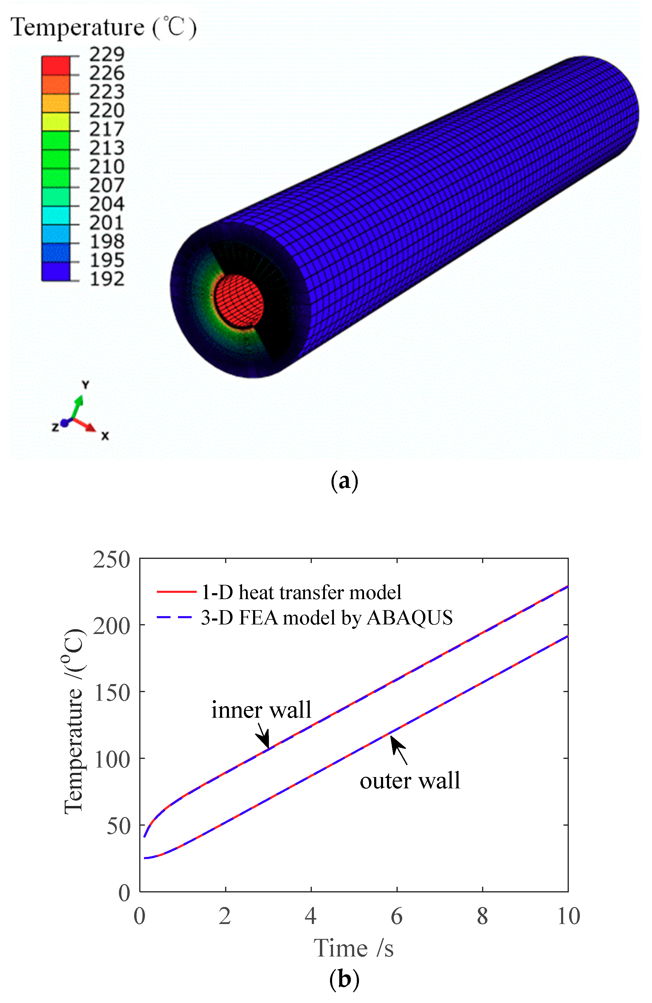
A grid-independent verification test of the numerical model was conducted. Considering the calculation accuracy and computational efficiency, the time step was set as $\Delta \tau$ = 0.1 s and the geometry was equally meshed into 1109 (N = 1100) parts in a 1D numerical model. When the mesh is further encrypted, and the time step is further reduced, the results have no effect on the temperature field. To further verify the numerical solution of the direct heat transfer model, it was compared with a 3D FEA thermal model of a gun barrel generated by ABAQUS software using the same parameters in Table 1. In the 3D FEA model, the element type was DC3D8 (eight node linear heat transfer brick element). The geometry was meshed into 314,160 elements. Fine meshes were applied near the inner wall due to the large temperature gradient, while more coarse meshes were arranged near the outer wall for the benefit of less computational time. In the finite element analysis (FEA) model, the inner wall was set to receive a uniform constant heat flux of $7\times {10}^5\mathrm{W}/{\mathrm{m}}^2$, which is consistent with the one-dimensional simplified model. No contact thermal resistance exists between the chrome and stainless steel layers. The axial length of the 3D gun barrel was 100 mm and the time period ($t_f$) was 10 s. The comparison result is shown in Figure 4.

5. Results and Discussions

In order to simulate the thermal conditions closer to the real situation, we used the data given by Chung et al. in Reference [37], which is an experimental heat transfer study for gun firing. We picked 16 main points from the profile of heat input (one round) in Figure 4 of Reference [37] using the software GetData Graph Digitizer v2.26 to generate two sets of arrays X and Y, which represent time and heat input, respectively. Heat input, Q [J/m²], is defined as the accumulated heat quantity over time per unit area. Then, these two arrays were fitted by using the “curve fitting tool” in MATLAB v2016a and obtain the following expression:

$$Q(t)=a_0\exp (-b_{0}t)+c_0$$

(19)

where the coefficients a₀, b₀ and c₀ are constant. The terms of time (t) and heat input (Q) are normalized as follows:

$$t^{\prime }=\frac{t}{\max (t)}$$

(20)

$$Q^{\prime }=\frac{Q}{\max (Q)}$$

(21)

Then, Equation (19) is further modified by

$$Q^{\prime }(t^{\prime })=a_1\exp (-b_1{t}^{\prime })+c_1$$

(22)

where the coefficients a₁, b₁ and c₁ are constant. The arrays ofX and Y are also normalized by dividing max(t) and max(Q), respectively.

The fitted data were compared with the original data given by Chung et al., as shown in Figure 5. Small offset are observed between the fitted function and D.Chung’s result, which is caused by the fitting error of RMSE 0.301and R-square 0.9899. The value of R-square is close to one, which indicates a good fitting result.

However, we can only obtain the heat input (Q) from Reference [37], while the boundary condition (Equation (2)) in our gun barrel thermal system requires the determination of heat flux (q) at each time moment. Heat flux, q [W/m²], is defined as the heat quantity per unit area per unit time. In this case, we fitted the curve of heat input (Q) against time in Figure 4 of Reference [37] and performed a first-order derivation of Q to time in order to gain the time-varying heat flux (q).

A first-order derivation of the heat input to the time item was then performed to obtain the heat flux, that is:

$$q(t^{\prime })=a_2\exp (-b_2{t}^{\prime })$$

(23)

According to the fitting result, $a_2=9.45\times {10}^5$ and $b_2=-5.712$. At the beginning of firing, we assume the heat flux reaches its maximum value linearly and quickly. Therefore, Equation (23) is further modified by:

$$q(t)=\{\begin{array}{ll}0& t_0\le t<t_1\\ 9.45\times {10}^5(t-t_1)/t_2-t_1& t_1\le t<t_2\\ 9.45\times {10}^5\exp (-5.712(t-t_2)/(t_3-t_2))& t_2\le t<t_3\end{array}$$

(24)

where the duration $[t_0,t_1]$ is the idle time and $[t_1,t_3]$ is the duration of heating. Here, we define $t_{\mathrm{dur}}(=t_3-t_0)$ to be the duration time of one-shot firing.

In practical engineering, measurement noises inevitably exist in the measured temperature. In our simulation, the simulated temperature measurements at specific sensor positions are generated by adding Gaussian white noise to the exact calculated temperature with a given boundary heat flux, that is:

$${(T_N^k)}_{\mathrm{mea}}={(T_N^k)}_{\mathrm{exa}}+\omega \sigma$$

(25)

where the subscript “mea” and “exa” are the measured and exact temperature, respectively, $\omega$ is a random variable over the range $-2.58\le \omega \le 2.58$ following a normal distribution with a zero mean and $\sigma$ is the standard deviation.

A series of numerical tests were performed to measure the accuracy and robustness of this inverse method and to identify the effects of measurement errors and future time step r on the inversion results. In order to evaluate the inversion results, the root-mean-square error (RMSE) and the average relative error of the estimated heat flux are defined by $S_q$ and ${\eta }_q$, respectively [38], shown as follows:

$$S_q=\sqrt{\frac{1}{K}{\displaystyle \sum _{k=1}^K{\left({(q^k)}_{\mathrm{exa}}-q^k\right)}^2}}$$

(26)

$${\eta }_q=\sqrt{\frac{1}{K}{\displaystyle \sum _{k=1}^K{\left({(q^k)}_{\mathrm{exa}}-q^k\right)}^2}}/\sqrt{\frac{1}{K}{\displaystyle \sum _{k=1}^K{\left({(q^k)}_{\mathrm{exa}}\right)}^2}}$$

(27)

where $K=M-r+1$.

5.1. Inverse Estimation of Gun Barrel Boundary Heat Flux

First, the accuracy of the proposed method was verified. The parameters were set as $t_0=0$, $t_1=1(\mathrm{s})$, $t_2=2(\mathrm{s})$, $t_3=14(\mathrm{s})$, and $t_{\mathrm{dur}}=14(\mathrm{s})$. The shooting time (t_dur) may vary with regard to different types of gun. In our paper, t_dur is chosen according to Reference [7]. The value of σ was set as zero (no noise) for a controlled condition. In the absence of measurement noise, a smaller value of r is chosen for model calibration. We take three different values of r (one, two, and three) to perform model calibration separately. When the future time step r takes from one to three, the estimated results are shown in Figure 6. It can be seen that the proposed inverse method can perfectly capture the heat flux profile under all given r values. In particular, when r=one an exact matching is obtained, and for r = two and r = three, a tiny deviation is observed at the peak point, which may be induced by the deterministic error of the SFSM algorithm. When r is small, the calculation process of SFSM can be considered to be approximately real time by using the temperature information in the ‘look-ahead’ time period of $r\Delta \tau$.

The corresponding error analysis of RMSE and average relative error are listed in

Table 2. Error analysis for heat flux inversion when no measurement noise is present.

Noise σ (°C)	Future Time Step r	RMSE Sq (W/m2)	Relative Error ηq (%)
0.00	1	619.60	0.21
0.00	2	4058.85	1.37
0.00	3	6407.32	2.15

. It shows high inversion accuracy with the maximum average relative error lower than 3%. The inversion error is slightly larger when r = three.

5.2. Effects of Measurement Noises on Inversion Results

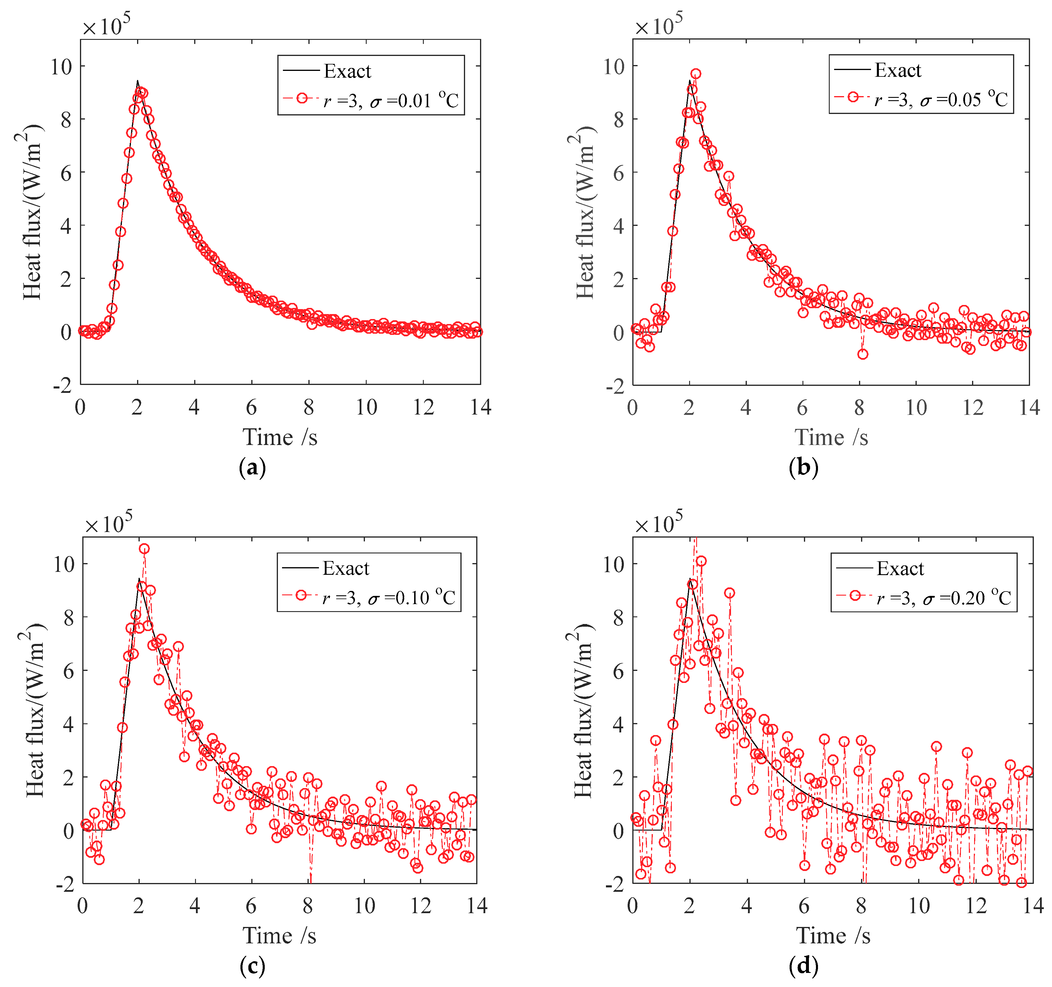
Secondly, the effects of measurement noise on the estimated results were investigated. The value of r was set as three and σ was set as 0.01, 0.05, 0.10, and 0.20 °C separately to represent different levels of measurement noise. The corresponding estimated heat fluxes are shown in Figure 7, and an error analysis is shown in

Table 3. Error analysis for heat flux inversion under different measurement noises.

Noise σ (°C)	Future Time Step r	RMSE Sq (W/m2)	Relative Error ηq (%)
0.01	3	11,369.88	3.82%
0.05	3	42,396.35	14.26%
0.10	3	82,716.89	27.82%
0.20	3	163,695.01	55.05%

. It was found that measurement noises have significant effects on the results. When the measurement error is small ($\sigma =0.01$ °C), the inversion result is good with a relative error lower than 4%. However, as the noise level increases, the fluctuation becomes more obvious, and a certain degree of oscillation occurs. For larger noise levels ($\sigma =0.10$ °C and $\sigma =0.20$ °C), the relative errors are up to 28% and 55%, which cannot meet the requirements of engineering application and need to be improved. The main reason for the above phenomenon is that IHTP is an ill-posed problem, for which the error of input signal will be greatly amplified in the output signal; therefore, effective regularization is needed to overcome this problem.

5.3. Effects of Future Time Step on Inversion Results

Thirdly, the impact of future time step (r) selection on the final results was investigated. The noise level was set at $\sigma =0.05$ °C, $\sigma =0.10$ °C, and $\sigma =0.20$ °C separately, and various values of r (3, 6 and 9) were taken for the numerical test. Figure 8 and

Table 4. Error analysis for heat flux inversion with various values of future time step (r).

Noise σ (°C)	Future Time Step r	RMSE Sq (W/m2)	Relative Error ηq (%)
0.05	3	42,396.35	14.26
	6	18,280.41	6.15
	9	36,267.48	12.20
0.10	3	82,716.89	27.82
	6	20,241.46	6.81
	9	36,148.26	12.16
0.20	3	163,695.01	55.05
	6	27,195.18	9.15
	9	36,224.85	12.18

show the effect of r on the inversion results of heat flux under different noise levels.

As seen from Figure 8, the future time step had noticeable effects on the estimated results of q(t). When r = three, the inversion results were unstable, exhibiting fluctuation or even oscillation; when r = six, the inversion results were greatly improved and the fluctuations were small; when r = nine, the inversion results were smooth and almost no fluctuations were observed, however the rapid change could not be captured. The corresponding error analysis is listed in Table 4. The inversion error was lower than 9.2% when r was six, and increased to 12% when r increased to nine.

The future time step r is an important parameter in SFSM. The value of r should be chosen to minimize the total error, which includes deterministic error and stochastic error [25,39]. The deterministic error is mainly produced by the assumption of heat flux form according to Equation (14); the stochastic error is the variance due to the amplification of measurement errors. A smaller value of r corresponds to a smaller deterministic error, but would make the inversion result more sensitive to measurement noise (especially when $\sigma$ is large), which enlarges the stochastic error, as shown in Figure 8. A larger value of r behaves like an average function to smooth the noisy profile (corresponding to smaller stochastic error), but also creates more deterministic errors so that some deviation is observed in the result of Figure 8. Therefore, a proper value of r is selected to minimize the total of these two errors. The simulation results show that when r is appropriately selected (r = six in our study), this method has minimum relative error and can achieve good regularization effect to overcome the ill-posedness of the inverse heat transfer problem.

5.4. Inverse Estimation of Boundary Heat Flux under Continuous Shooting

Considering the fact that there are rapid continuous shooting processes in practical engineering applications, in the present study, the impact of shooting duration time and continuous shooting process on the inversion results were investigated. Two sets of different shooting duration time, t_dur = 7 s and t_dur = 14 s, were considered. According to Equation (23), the forms of heat flux profile for one shot with durations of 7 s and 14 s were defined as follows:

$$q(t)=\{\begin{array}{ll}0& 0\le t<0.5\mathrm{s}\\ 2\times 9.45\times {10}^5(t-0.5)& 0.5\mathrm{s}\le t<1\mathrm{s}\\ 9.45\times {10}^5\exp \left(-0.952(t-1)\right)& 1\mathrm{s}\le t\le 7\mathrm{s}\end{array}$$

(28)

$$q(t)=\{\begin{array}{ll}0& 0\le t<1\mathrm{s}\\ 9.45\times {10}^5(t-1)& 1\mathrm{s}\le t<2\mathrm{s}\\ 9.45\times {10}^5\exp \left(-0.476(t-2)\right)& 2\mathrm{s}\le t<14\mathrm{s}\end{array}$$

(29)

For continuous three-shot firing, if we assume the interval between shots is very short and neglected, the heat flux form is periodically changing by repeating the wave form defined by Equation (28) or (29). The numerical tests were conducted by setting σ = 0.10 °C and r = 6. The inversion results are shown in Figure 9. From Figure 9a, it can be seen that the estimated heat flux is very close to the exact profile except for some clear deviation found at the peak where heat flux has a sharp and rapid change. From Figure 9b, it can be seen that the deviation was smaller when the firing duration was 14 s. An error analysis is shown in

Table 5. Error analysis for heat flux inversion under continuous shooting.

Noise σ (°C)	Future Time Step r	Duration Time tdur (s)	RMSE Sq (W/m2)	Relative Error ηq (%)
0.10	6	7	50,241.69	16.85
0.10	6	14	22,657.52	7.62

. For t_dur = 7 s, the average relative error was up to 16.9%, while for t_dur = 14 s, the average relative error reduced to 7.6%, which is similar to the error level of single wave inversion.

The above results show that the inversion method of this paper can accurately track the periodic heat flux changes without oscillating. However, fast changing heat flux wave can cause degradation of estimation accuracy. The reason for this is that, although a larger value of r can smooth the inversion result, it creates deterministic error and is likely to cause some information of rapid heat flux changes to be lost. When the measurement noise is large, the inversion results might be improved by adjusting the value of a future time step r and step size ∆τ.

6. Conclusions

In this study, an inverse method was developed to estimate the unknown boundary heat flux on the inner wall of two-layer gun barrel during shooting process. This method couples the finite difference method and the sequential function specification method, and can achieve quick and efficient identification of unknown time-variant heat flux. The results of numerical tests show that the proposed method has high inversion accuracy, and the following conclusions can be drawn: (1) The method can accurately track the time-varying heat flux profile during one-shot and three-shots continuous shooting without oscillating; and (2) the measurement noises have a significant effect on the inversion results. By selecting a proper r value, this method has good regularization characteristic to effectively suppress the adverse effects of measurement noise; and (3) a low-noise, high-accuracy temperature data and smaller value of r are preferred to capture rapid heat flux changes over time.

Our work can be further extended to visualize the 3D transient temperature field for gun barrel. In the future, the method developed in this study is expected to be useful in solving the transient inverse heat transfer problem where time-varying heat flux or temperature cannot be measured at one of the boundaries.