Energetical Analysis of Two Different Configurations of a Liquid-Gas Compressed Energy Storage

Abstract

In order to enhance the spreading of renewable energy sources in the Italian electric power market, as well as to promote self-production and to decrease the phase delay between energy production and consumption, energy storage solutions are catching on. Nowadays, in general, small size electric storage batteries represent a quite diffuse technology, while air liquid-compressed energy storage solutions are used for high size. The goal of this paper is the development of a numerical model for small size storage, environmentally sustainable, to exploit the higher efficiency of the liquid pumping to compress air. Two different solutions were analyzed, to improve the system efficiency and to exploit the heat produced by the compression phase of the gas. The study was performed with a numerical model implemented in Matlab, by analyzing the variation of thermodynamical parameters during the compression and the expansion phases, making an energetic assessment for the whole system. The results show a good global efficiency, thus making the system competitive with the smallest size storage batteries.

1. Introduction

The rise in the energy demand in recent years has led to an increase in the development and use of renewable energy sources throughout the world. Since the production of energy from renewable sources is intermittent because it depends on weather conditions, the storage of electricity and heat is of considerable and growing importance. Energy storage technologies are gaining much attention due to their ability to level electrical loads, to manage and compensate for the intermittent nature of renewable energies according to the demand of the various users and also to store excess power during the day and move closer to energy self-sufficiency. Various energy storage technologies can be classified for different physical operating principles, although according to the different final applications it is necessary to choose the most advantageous type of storage. In general, according to the 2016 report [1], 170 GW of energy storage have been installed in the world and Italy currently (with 7 GW) is among the top ten countries in the world. For what concerns installed technologies, 95% are mechanical while their applications are not in the residential sector but the network services and energy dispatching since the costs of technology are still not sustainable. Nowadays, in EU countries, the storage solutions in the residential sector are spreading especially for new buildings developed according to the “fully electric” concept. Among the common types of storage, hydroelectric pumping is certainly the most widespread, even if its strong dependence on the morphology of the place will limit its further development in favor of other technologies such as compressed air storage. In the residential sector, electrochemical accumulation is the most common technology. However, in the future, the compressed air storage could be a viable solution thanks to reliability, low environmental impact, and energy self-sufficiency. The idea of storing electricity using compressed air dates back to the early 1940s, although until the 1960s the development of the CAES (Compressed Air Energy Storage) was not pursued either in research or in the industrial sector. The first installation took place in Germany in 1969 with the Huntorf plant thanks to appropriate geological formations to accumulate large quantities of compressed gas. Nowadays, there are two large size plants like Huntfort and Alabama [2], while for the small size plants, a system with vessel or pipe [3,4,5], has replaced the natural cave. In general, CAES technology suffers from very low efficiencies, due to losses in the compressor and turbine [5,6,7,8] and a very high cost, higher than $120/Kwh [3]. At the same time, it is a desirable technology due to its low environmental impact, its very high life cycle and, above all, its ability to recover thermal energy, attracting much scientific research. In general, CAES systems can be divided into three macro-categories: diabatic, adiabatic and isothermal [9]. In the first type (D-CAES) the heat associated to the compression phase is lost in the environment during the cooling phase, so it is necessary to use an external heat source for the discharge process. In the second type (A-CAES) the heat of the compression phase is collected and used to preheat the air, before the expansion. In the third configuration (I-CAES), the heat produced during the compression phase is reused for other connected applications. Sciacovelli et al. [10] in the paper show that the round-trip efficiency grows of 25% when the thermal storage is used to help the CAES process to maintain the adiabatic conditions. There are also hybrid CAES systems with a liquid air energy storage (LAES) [11]. In these systems the advantages are higher efficiency, lower costs and high energy densities. The most critical challenges regarding CAES technology are the management of the heat produced during the compression of the gas and the increase of the efficiency of the system. For this reason, many studies have been performed about the possible achievement of isothermal or almost isothermal compressions through the use of liquids in the form of a spray during compression [12,13,14,15,16,17,18]. This type of CAES, on the one hand, increases the efficiency of the system, increasing the efficiency of compression, on the other manages to recover heat in the compression phase for other uses, thus making the technology CAES a fundamental technology to reach self-sufficient energy.

In the last years, another relevant field of applications for the CAES technologies is to use the small-scale energy output for commercial and residential buildings and for individual stand-alone applications [19,20]. Potential and performance evaluations of CAES have been mainly made by simulation tools or modeling processes to have energy and exergy results [21]. In general, to study the CAES system, most of the research use the simulated data of CAES with simulated data of the end users such as an apartment or buildings and only a few papers proposed an economic analysis [22].

Another significant development of the CAES system is the liquid -gas compressed air energy storage. The idea of this system born to improve the efficiency of the system, because it is more efficient to pump the liquid than the air inside of the vessel. In the literature, Odukomaiya et al. [23] analyze this particular CAES system. Our idea is to use this system for small energy applications, where it is necessary to obtain self-sufficient energy. The system involves the compression of a gas inside a tank through the introduction of a liquid that is pumped into the tank through a hydraulic pump whose efficiency is higher than an air compressor. The storage system is then loaded by pumping the liquid into the tank, with the consequent reduction in the volume of the gas and the relative increase in terms of pressure energy. When the user requires electric power, the high-pressure liquid is expanded using a Pelton turbine coupled to an electric generator. During this phase, the volume of gas inside the tank expands, and the pressure decreases (Figure 1). Two different configurations of the gas-liquid storage system have been studied, with the aim of assessing how to use the heat produced during the compression phase. In a first configuration the heat produced by compression will not be reused; in the second one, a liquid will be injected into the gas using a spray to increase the efficiency of the system.

2. Description of the Configurations

The studied system allows compressed air to be stored in high-pressure tanks, using a high-efficiency hydraulic pump instead of compressor usually used in storage systems. The system, as shown in Figure 1, is loaded by pumping water into the tank thus reducing the available gas volume. As a result, the temperature and gas pressure increase. After the compression, there is a transitory phase during which all the thermodynamic variables stabilize. When electricity demand occurs, high-pressure water is released into a Pelton turbine coupled to a high efficiency electric generator, thus producing electricity. During the discharge phase, the volume of gas expands and the pressure consequently decreases. The pump used to pressurize the tank is of the “PD” type (positive displacement). This on purpose designed pump allows particular applications where low flow rates and pressures up to 200–300 bar are required. The efficiency of the considered hydraulic machines can reach a value of 90%, and they result commercially available on a large scale (1–500 kW). For what concerns the tank, high-pressure resistant models (over 300 bar) are available on the market in a volume range between 10 and 1000 L. The adopted configurations are shown in Figure 2.

The first, named “first configuration,” has been described above and is the simplest scheme among those proposed. That named “second configuration” differs from the first because of the presence of a device that atomizes the water inside the tank. The reason for this solution lies in the fact that through this nebulization it is possible to consider the transformation as isentropic, in order to increase the overall efficiency.

3. Mathematical Model

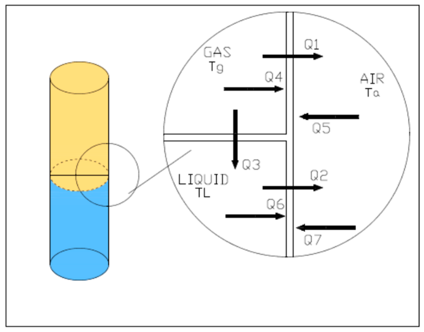
In order to better understand the mathematical model implemented it is possible to start from the analysis of Figure 3. The equations related to heat transfer are the following:

$${\dot{Q}}_1=U{A}_G(T_G-T_{amb})$$

(1)

$${\dot{Q}}_2=U{A}_L(T_L-T_{amb})$$

(2)

$${\dot{Q}}_3=h_{G,L}{A}_{G,L}(T_G-T_L)$$

(3)

$${\dot{Q}}_4=h_{i,G}{A}_{i,G}(T_G-T_{T,G})$$

(4)

$${\dot{Q}}_5=h_o{A}_{o,G}(T_{T,G}-T_{amb})$$

(5)

$${\dot{Q}}_6=h_{i,L}{A}_{i,L}(T_G-T_{T,L})$$

(6)

$${\dot{Q}}_7=h_o{A}_{o,L}(T_{T,L}-T_{amb})$$

(7)

From these expressions, for each configuration studied, the thermal balances were evaluated both during the charge phase both during the discharge phase and obviously during the injection phase.

To develop the mathematical model some assumptions has been done:

-

Inside of the liquid and gas respectively the temperature is uniform;

-

Air temperature of the environment is constant;

-

Thermophysical properties of the tank constant;

-

The gas inside of the tank follow the ideal gas law;

-

All processes occurring at quasi-steady state;

-

Negligible heat transfer between the tank upper (TG) and tank lower (TL).

To model the transient thermodynamic response of the system, in the Equation (8) we analyze the energy exchange inside of the gas.

$$m_{G}Cv\frac{d{T}_G}{dt}=-h_{G,L}{A}_{G,L}(T_G-T_L)-U{A}_G(T_G-T_{amb})-p_G\frac{d{V}_G}{dt}$$

(8)

The term on the left is the time rate of change of the energy contained within the gas; the first term on the right side of the equation is the net rate of the thermal energy transferred from the gas to the liquid; the second term is the net rate of the thermal energy transferred from the gas to the external environment through the tank walls and the last term is the net rate at which energy is transferred out by boundary work. The last term does not appear during the pause phase for obvious reasons.

The Equation (9) is the energy equation for the liquid.

$$m_{L}C{v}_L\frac{d{T}_L}{dt}=h_{G,L}{A}_{G,L}(T_G-T_L)-U{A}_L(T_L-T_{amb})+{\dot{m}}_{L}C{v}_L(T_{amb}-T_L)$$

(9)

The term on the left side of the equation represent the time rate of change of the energy contained within the liquid; the first term on the right side is the net rate of the thermal energy transferred from the liquid to gas; the second term is the net rate of the thermal energy transferred from the liquid to external environment through the tank walls; and the last term is the net rate of energy transfer inside of the liquid accompanying mass flow.

The Equation (10) is the energy equation for the tank walls in contact with the gas

$$m_{T,G}C{v}_T\frac{d{T}_{T,G}}{dt}=h_{i,G}{A}_{i,G}(T_G-T_{T,G})-h_o{A}_{o,G}(T_{T,G}-T_{amb})$$

(10)

The term on the left side of the equation is the time rate of change of the energy contained within the corresponding mass; the first term on the right is the net rate of the thermal energy transferred from the gas to the tank, the second term is the net rate of the thermal energy transferred from the tank to the external environment.

The Equation (11) is the energy equation for the tank walls in contact with liquid.

$$m_{T,L}C{v}_T\frac{d{T}_{T,L}}{dt}=h_{i,L}{A}_{i,L}(T_L-T_{T,L})-h_o{A}_{o,L}(T_{T,L}-T_{amb})$$

(11)

The term on the left side of the equation is the time rate of change of the energy contained within the corresponding mass; the first term on the right is the net rate of the thermal energy transferred from the liquid to the tank and the second term is the net rate of the thermal energy transferred from the liquid to the external environment.

Equation (12) is the continuity equation for the gas

$$\frac{d{V}_G}{dt}=-\frac{\dot{m_L}}{{\varrho }_L}$$

(12)

Equation (13) is the continuity equation for the liquid.

$$\frac{d{m}_L}{dt}=\dot{m_L}$$

(13)

To study the second configuration more equations are utilized, in particular, the following equations are utilized to model the effect of the direct-contact heat exchange between the gas and the liquid obtained via spraying [23].

Regarding this phenomena, it is essential to explain that for this high pressure inside of the tank, the evaporation of the liquid is minimal and then the liquid-gas mass diffusion has been neglected.

In the model, we assumed that the single droplet falls at a constant velocity and the Equation (14) show the velocity of the single droplet.

$$v_{term}=\sqrt{\frac{4g{D}_{dr}{\varrho }_{dr}}{3{\varrho }_G{C}_D}}$$

(14)

Obtaining the terminal velocity allows for the calculation of the droplet travel time or residence time in the gas using Equation (15)

$$t_{trav}=\frac{l\left(t\right)}{v_{term}}$$

(15)

where the l(t) is the distance from the top of the tank and the liquid below.

Equation (16), show how we can calculate the number of the droplets generated per unit time.

$${\dot{N}}_{dr}=\frac{6{\dot{V}}_{spr}}{\pi D^3{}_{dr}}$$

(16)

Using the value of the time travel obtained from Equation (15) and the number of the droplets generated per unit time (Equations (16) and (17)) shows how we can calculate the total number of droplets of liquid traveling through the gas.

$$N_{dr}={\dot{N}}_{dr}{t}_{trav}$$

(17)

With the Equation (18) we can calculate the trend of the temperature of the droplets during the time from the exit of the nozzle in the upside of the tank to the bottom side of the tank

$$\frac{T_{dr,out}-T_G}{T_{dr,in}-T_G}=e^{-\frac{t_{trav}}{{\tau }_{dr}}}$$

(18)

Equation (19) show the thermal time constant of the liquid droplet.

$${\tau }_{dr}=\frac{{\varrho }_{dr}{V}_{dr}{C}_{dr}}{h_{dr}{A}_{s,dr}}$$

(19)

Equation (20) shows the Nusselt number, utilizing the relation of Ranz and Marshall.

$$N{u}_{dr}=2+0.6R{e}^{1/2}P{r}^{1/3}$$

(20)

Then in the Equation (21), the resulting heat transfer coefficient is calculated:

$$h_{dr}=\frac{Nu{k}_{dr}}{D_{dr}}$$

(21)

The heat loss (or gain) from the drops can be calculated using Equation (22), that how we can see depends from the temperatures of the drops as they enter and leave of the gas.

$$Q_{dr}={\varrho }_{dr}{V}_{dr}{c}_{dr}(T_{dr,out}-T_{dr,in})$$

(22)

The rate of heat loss from the entire spray is then calculated as follows in Equation (23)

$${\dot{Q}}_{spr}={\dot{N}}_{dr}{Q}_{dr}$$

(23)

To calculate the effect of the droplets on the temperature of the bulk liquid at the bottom of the tank the mixing Equation (24) is utilized. At each time step, the enthalpy of the drops plus the enthalpy of the bulk liquid must equal to the enthalpy of the combined liquid mixture

$$T_{L,mixed}=\frac{{\dot{m}}_{spr}\Delta t{C}_{dr}{T}_{dr}+m_L{C}_L{T}_L}{({\dot{m}}_{spr}\Delta t+m_L)C_L}$$

(24)

The presence of the droplets inside of the gas will change the heat transfer during the charging and discharging phases. Then the Equations (8) and (9) will change in the second configuration in the Equation (25) for the gas and Equation (26) for the liquid.

$$m_{G}Cv\frac{d{T}_G}{dt}=-h_{G,L}{A}_{G,L}(T_G-T_L)-U{A}_G(T_G-T_{amb})-p_G\frac{d{V}_G}{dt}-{\dot{Q}}_{spr}$$

(25)

$$\begin{gathered} m_{L}C{v}_L\frac{d{T}_L}{dt}=h_{G,L}{A}_{G,L}(T_G-T_L)-U{A}_L(T_L-T_{amb})+{\dot{m}}_{L}C{v}_L(T_{amb}-T_L) \\ +{\dot{m}}_{spr}C{v}_L(T_G-T_L) \end{gathered}$$

(26)

The efficiency of the studied system is calculated as follows:

$${\eta }_{ind}=\frac{{{{\displaystyle \sum }}_{j=1}^N{p}_j(V_{g,j+1}-V_{g,j})}_{discharge}}{{{{\displaystyle \sum }}_{j=1}^N{p}_j(V_{g,j+1}-V_{g,j})}_{charge}}$$

(27)

where N = 20 is the number of time steps of charging and discharging phases.

4. Results and Discussion

Let’s start by analyzing what happens in the first configuration. The initial parameters of this configuration are reported in

Table 1. Parameter utilized for the first configuration.

Parameter	Value
Vser	1.98 m3
mc	178.14 kg
$\dot{m_l}$	0.58333 kg/s
t	20 min
U	8.3 W/(m2K)
tpausa	720 min (12 ore)
Piniz	78 bar
Tamb	298.15 K
TG,iniz	298.15 K
TL,iniz	298.15 K

.

In order to better understand the energy performance of the two configurations, several simulations have been implemented. In each simulation explained in the table to make a detailed sensitivity analysis of the system (

Table 2. Description of the Simulations implemented.

Description	Value
SIM 1	$\dot{m}$ = 0.5833 kg/s
SIM 2	$\dot{m}$ = 0.865 kg/s
SIM 3	$\dot{m}$ = 1.166 kg/s
SIM 4	V = 1.98 m3
SIM 5	V = 2.97 m3
SIM 6	V = 3.96 m3
SIM 7	U = 8.3 W/m2K
SIM 8	U = 1.5 W/m2K
SIM 9	U = 1 W/m2K
SIM 10	t = 20 min
SIM 11	t = 10 min
SIM 12	t = 5 min

).

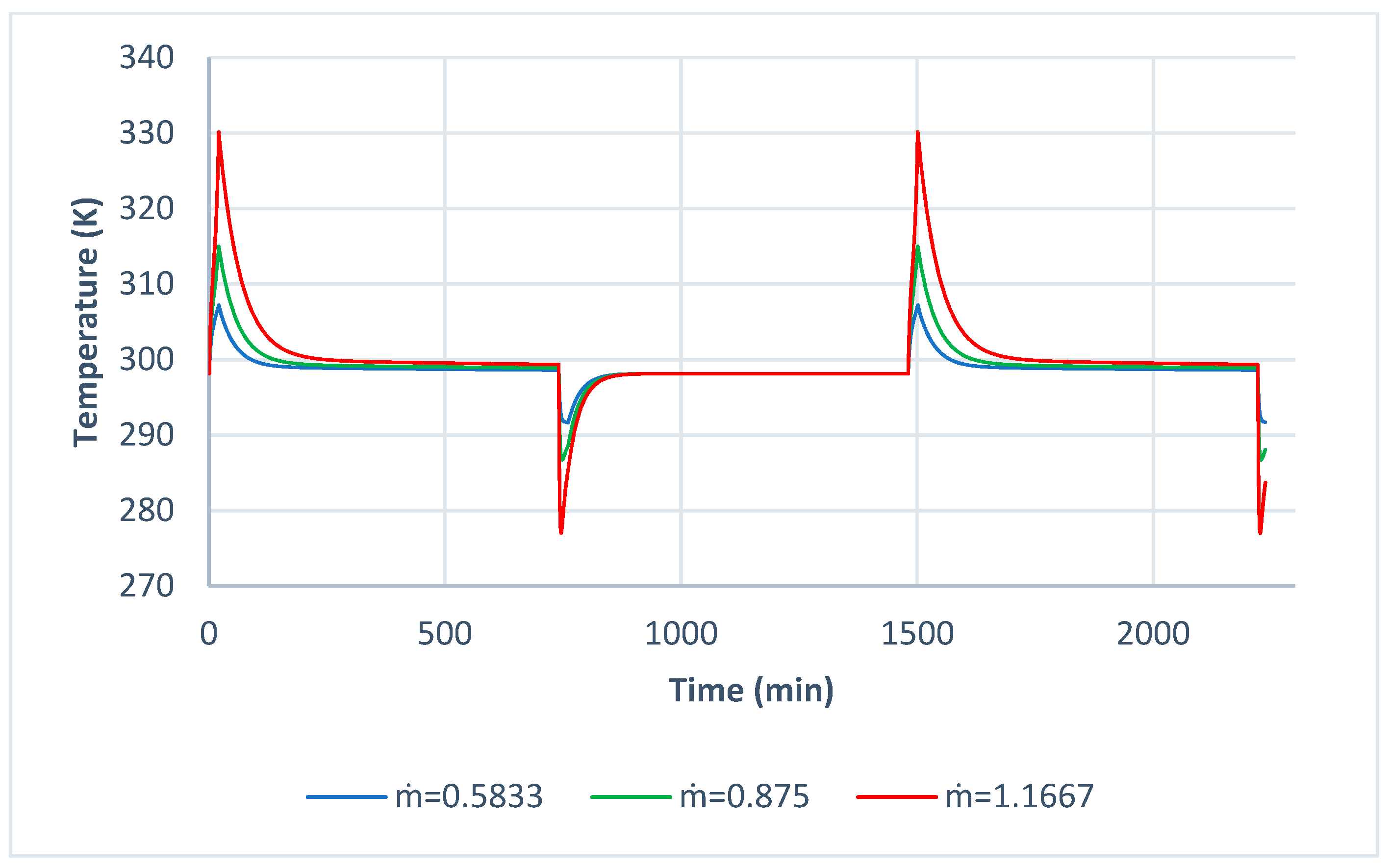
Below are presented the graphs of the first configuration and the second configuration for the 12 simulations performed. The time step assumed during the calculation is equal to 60 s, decreasing of step size do not influence the obtained value of system efficiency. The charging and discharging phases take 20 min In Figure 4 and Figure 5 the variation of the temperature of the gas inside the tank was evaluated for three different values of the liquid flow rate respectively for the first and second configuration.

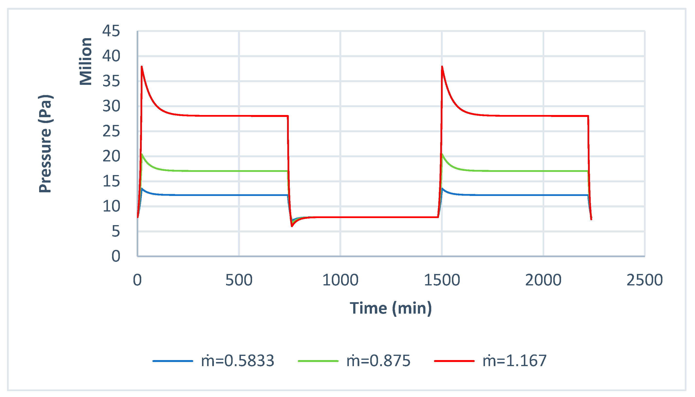
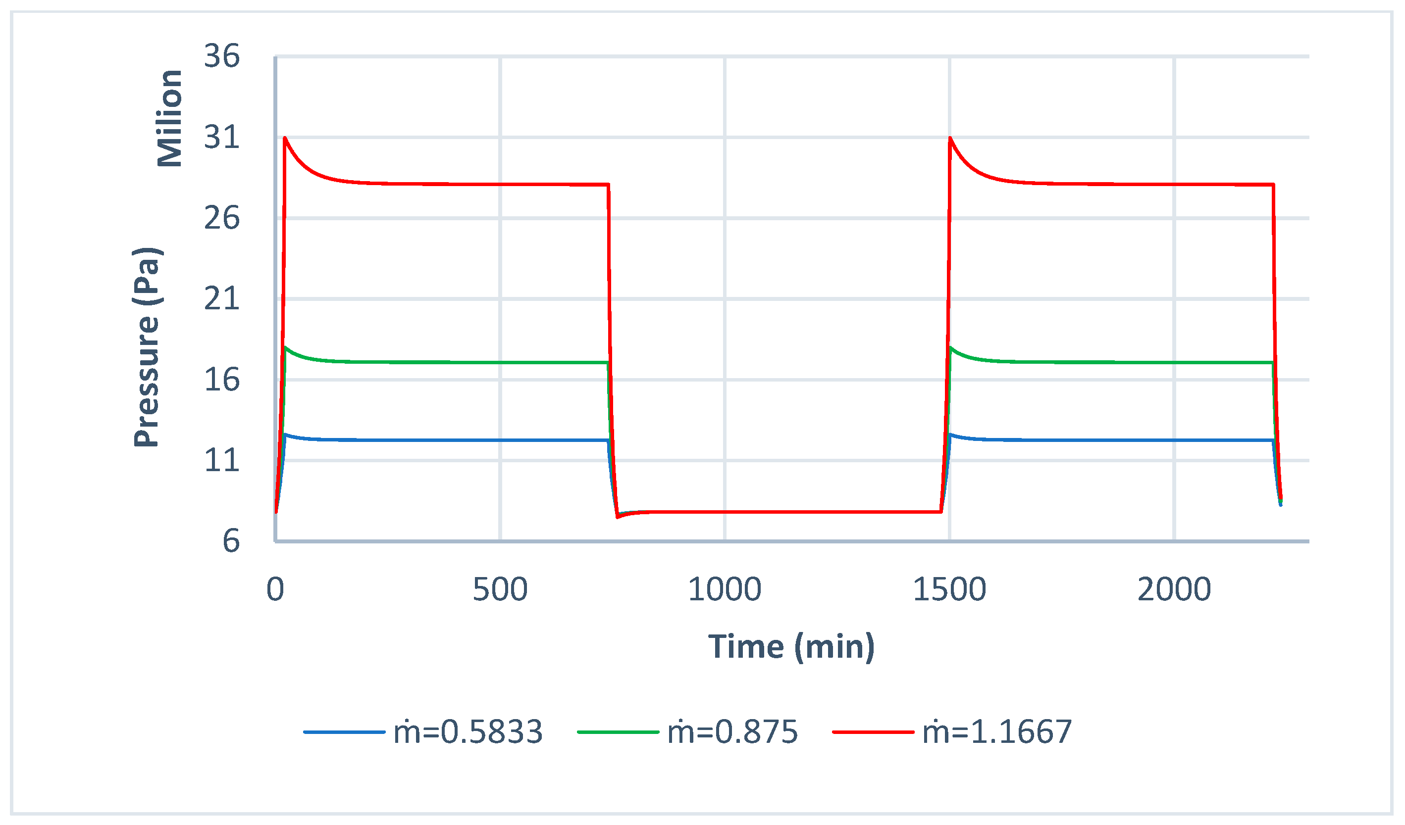
In Figure 6 and Figure 7 the variation of the pressure of the gas inside of the tank was evaluated for three different values of the liquid flow rate respectively for the first and second configuration.

Table 3. Efficiency system for the first configuration varying the liquid flow rate.

Efficiency	$\dot{\mathit{m}}$ = 0.5833 kg/s	$\dot{\mathit{m}}$ = 0.875 kg/s	$\dot{\mathit{m}}$ = 1.167 kg/s
ηind (%)	89.7	82.5	72.5

shows the values of the system efficiency for the first configuration varying the liquid flow rate. It can be seen that the efficiency increases when the mass flow rate decrease.

Table 4. Efficiency system for the second configuration varying the liquid flow rate.

Efficiency	$\dot{\mathit{m}}$ = 0.5833 kg/s	$\dot{\mathit{m}}$ = 0.875 kg/s	$\dot{\mathit{m}}$ = 1.1667 kg/s
ηind (%)	96.1	93.4	89.1

show the values of the efficiency system for the second configuration varying the liquid flow rate. It can be seen that the efficiency increases when the mass flow rate decrease.

In Figure 4, Figure 5, Figure 6 and Figure 7 it is possible to see that as the entering water mass flow increases, both the pressure and the temperature of the gas increase. From figures, we can note that the in the first configuration the values of the temperature and the gas are higher than in the second configuration.

Using $\dot{m}$ = 0.875 kg/s for the first configuration would seem to be the best choice, since a final pressure of the charge phase around 200 bar shows a significant increase in the temperature of the gas (up to 360 K), while maintaining a significant efficiency (82.5%). The same reasoning, we can have done for the second configuration. Taking the $\dot{m}$ = 1.167 kg/s guarantees higher values of temperature but also high pressure to withstand for the tank (thus increasing construction costs). The first configuration simulation setting also presents decidedly lower efficiency with respect to the second configuration., where the efficiency are considerably higher (Table 4).

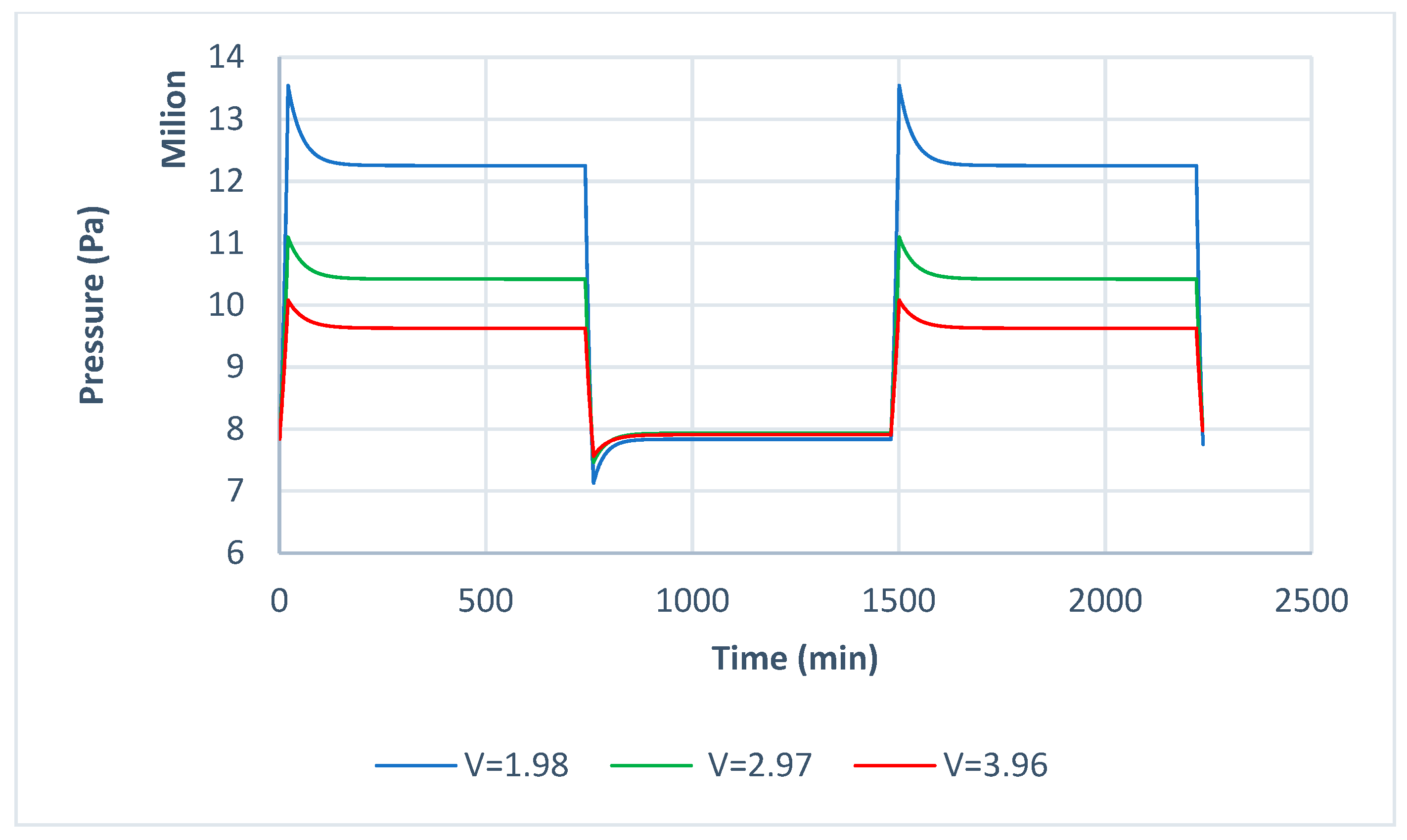
Subsequently, it was decided to change the volume of the tank. Figure 8, Figure 9, Figure 10 and Figure 11 shows the temperature and pressure inside of the tank for the first and second configuration respectively varying the volume of the thank.

The Figure 8, Figure 9, Figure 10 and Figure 11 show that as the volume of accumulation increases, a reduction in gas pressure and temperature is obtained for both configurations.

In

Table 5. Efficiency system for the first configuration varying the Volume of the tank.

Efficiency	V = 1.98 m3	V = 2.97 m3	V = 3.96 m3
ηind (%)	89.7	93.45	95.2

and

Table 6. Efficiency system for the second configuration varying the Volume of the tank.

Efficiency	V = 1.98 m3	V = 2.97 m3	V = 3.96 m3
ηind (%)	96.1	96.9	97.4

, are reported the values of the efficiency varying the volume of the tank respectively for the first and second configuration.

In tables are evident that when the volume of the thank increases the value of the efficiency for both configurations but with slighter efficiency for the first configuration.

Figure 12, Figure 13, Figure 14 and Figure 15 show how the temperature and the pressure of the gas inside of the thank varies for three different values of the transmittance of the thank.

Figure 12, Figure 13, Figure 14 and Figure 15 shows that as the transmittance decreases a significant increase in pressure and temperature occurs thanks to the higher isolation of the tank walls with respect to the external environmental conditions. Furthermore, the transient phase during which the pressure and temperature values tend to stabilize is extended. The efficiency, on the other hand, decreases by almost one percentage point (

Table 7. Efficiency system for the first configuration varying the transmittance of the tank.

Efficiency	U = 8.3 W/(kg·K)	U = 1.5 W/(kg·K)	U = 1 W/(kg·K)
ηind (%)	89.7	89	89

and

Table 8. Efficiency system for the second configuration varying the transmittance of the tank.

Efficiency	U = 8.3 W/(kg·K)	U = 1.5 W/(kg·K)	U = 1 W/(kg·K)
ηind (%)	96.1	96.14	96.15

).

Then, the variation in temperature and pressure was evaluated as a function of the charging time (Figure 16, Figure 17, Figure 18 and Figure 19).

Figure 16, Figure 17, Figure 18 and Figure 19 show that a reduction of the charge and discharge phase results in a significant decrease in both pressure and gas temperature for the first and second configuration. The efficiency increases considerably, but the amount of work that can be extracted decreases drastically (

Table 9. Efficiency system for the first configuration varying the charging time.

Efficiency	T = 20 min	T = 10 min	T = 5 min
ηind (%)	89.7	94.8	97.4

and

Table 10. Efficiency system for the second configuration varying the charging time.

Efficiency	T = 20 min	T = 10 min	T = 5 min
ηind (%)	96.1	97.2	98.1

). Therefore, reducing the charge and discharge time does not entail any real advantage to the system, somewhat it limits its potential.

5. Conclusions

Energy storage technologies are destined to be increasingly important within the so-called “smart grids.” Nowadays, CAES represent a valid solution thanks to their reliability, their possible integration with renewable energies and their ability to integrate themselves into poly-generation systems. Among the various types and models of CAES studied since the 40s till today, the Gas-Liquid Energy Storage (GLES) can be a turning point. In fact, they are scalable systems able to reach high pressures, with a high energy density and low environmental impact. The last feature puts them in an advantageous position compared to the batteries, which nowadays represent the primary system of accumulation on a small scale. Also, the batteries have the ability to accumulate only electricity, while with GLES, it is possible to store electricity and heat, recovering and allocating it to other purposes (such as domestic hot water or air conditioning systems).

In the first configuration, with the initialization parameters, it can be seen that in 20 min of time charge, high pressures are reached (slightly above 135 bar), gas temperature around 330 K and an indicated yield of 89.7%. The sensitivity analysis highlighted how the increase in the mass flow of water entering the tank entails a substantial increase in pressure and temperature, while the increase in the volume of accumulation causes an opposite effect. The decrease in transmittance, instead, has as the main effect the increase in the short interval during the pause phases, due to a better isolation of the tank. Moreover, a decrease in charge and discharge times does not bring significant benefits to the system.

In the second configuration, the substantial constructive difference due to the presence of the nebulizer leads to entirely different results. The presence of the droplets sprayed inside the tank causes the temperature to drop during the charging phase and rise during the discharge. The main consequence of the presence of the sprayer is a considerable increase in yield: in fact, it goes from 89.7% of the first configuration to 96.1% of the second; this is due to a reduction in the work required and an increase in the work extracted.

References

- Di Milano, P. Facoltà di Ingegneria Gestionale, Energy Storage Report; Politecnico di Milano: Milan, Italy, November 2016. [Google Scholar]
- Madlener, R.; Latz, J. Economics of centralized and decentralized compressed air energy storage for enhanced grid integration of wind power. Appl. Energy 2011, 101, 299–309. [Google Scholar] [CrossRef]
- Luo, X.; Wang, J.; Dooner, M.; Clarke, J. Overview of current development in electrical energy storage technologies and the application potential in power system operation. Appl. Energy 2015, 137, 511–536. [Google Scholar] [CrossRef]
- Díaz-González, F.; Sumper, A.; Gomis-Bellmunt, O.; Villafáfila-Robles, R. A review of energy storage technologies for wind power applications. Renew. Sustain. Energy Rev. 2012, 16, 2154–2171. [Google Scholar] [CrossRef]
- Mahlia, T.M.I.; Saktisahdan, T.J.; Jannifar, A.; Hasan, M.H.; Matseelar, H.S.C. A review of available methods and development on energy storage; technology update. Renew. Sustain. Energy Rev. 2014, 33, 532–545. [Google Scholar] [CrossRef]
- De Lieto Vollaro, R.; Faga, F.; Tallini, A.; Cedola, L.; Vallati, A. Energy and thermodynamical study of a small innovative compressed air energy storage system (micro-CAES). Energy Procedia 2015, 82, 645–651. [Google Scholar] [CrossRef]
- Tallini, A.; Vallati, A.; Cedola, L. Applications of micro-CAES systems: Energy and economic analysis. Energy Procedia 2015, 82, 797–804. [Google Scholar] [CrossRef]
- Vallati, A.; Grignaffini, S.; Romagna, M. A new method to energy saving in a micro grid. Sustainability 2015, 7, 13904–13919. [Google Scholar] [CrossRef]
- Venkataramani, G.; Parankusama, P.; Ramalingam, V.; Wang, J. A review on compressed air energy storage—A patway for smart grid and polygeneration. Renew. Sustain. Energy Rev. 2016, 62, 895–907. [Google Scholar] [CrossRef]
- Sciacovelli, A.; Li, Y.; Chen, H.; Wu, Y.; Wang, J.; Garvey, S.; Ding, Y. Dynamic simulation of Adiabatic Compressed Air Energy Storage (A-CAES) plant with integrated thermal storage link between components performance and plant performance. Appl. Energy 2017, 185, 16–28. [Google Scholar] [CrossRef]
- Morgan, R.; Nelmes, S.; Gibson, E.; Brett, G. Liquid air energy storage—Analysis and first results from a pilot scale demonstration plant. Appl. Energy 2015, 137, 845–853. [Google Scholar] [CrossRef]
- LightSail Energy. Technology. Available online: http://www.lightsail.com (accessed on 3 December 2018).
- Sustain, X. SustainX’s ICAES. Available online: http://www.sustainx.com/technology-isothermal-caes.htm (accessed on 3 December 2018).
- Kim, Y.M.; Favrat, D. Energy and exergy analysis of a micro-compressed air energy storage and air cycle heating and cooling system. Energy 2010, 35, 213–220. [Google Scholar] [CrossRef] [Green Version]
- Facci, A.L.; Sánchez, D.; Jannelli, E.; Ubertini, S. Trigenerative micro compressed air energy storage: Concept and thermodynamic assessment. Appl. Energy 2015, 158, 243–254. [Google Scholar] [CrossRef]
- Li, Y.; Wang, X.; Li, D.; Ding, Y. A trigeneration system based on compressed air and thermal energy storage. Appl. Energy 2012, 99, 316–323. [Google Scholar] [CrossRef]
- Vallati, A.; Grignaffini, S.; Romagna, M.; Mauri, L. Effects of different building automation systems on the energy consumption for three thermal insulation values of the building envelope. In Proceedings of the 2016 IEEE 16th International Conference on Environment and Electrical Engineering EEEIC, Florence, Italy, 7–10 June 2016. [Google Scholar]
- Ocłoń, P.; Bittelli, M.; Cisek, P.; Kroener, E.; Pilarczyk, M.; Taler, D.; Rao, R.V.; Vallati, A. The performance analysis of a new thermal backfill material for underground power cable system. Appl. Thermal Eng. 2016, 108, 233–250. [Google Scholar] [CrossRef]
- Jannelli, E.; Minutillo, M.; Lubrano Lavadera, A.; Falcucci, G. A small-scale CAES (compressed air energy storage) system for standalone renewable energy power plant for a radio base station: A sizing design methodology. Energy 2014, 78, 313–322. [Google Scholar] [CrossRef]
- Castellani, B.; Morini, E.; Nastasi, B.; Nicolini, A.; Rossi, F. Small-scale Compressed Air Energy Storage Application for renewable Energy Integration in a Listed Building. Energies 2018, 11, 1921. [Google Scholar] [CrossRef]
- Kim, Y.; Lu, K.; Ma, L.; Wang, J.; Dooner, M.; Miao, S.; Li, J.; Wang, D. Overview of compressed Air Energy Storage and Technology Development. Energies 2017, 10, 991. [Google Scholar] [CrossRef]
- Gu, Y.; McCalley, J.; Ni, M.; Bo, R. Economic modelling of Compressed Air Energy Storage. Energies 2013, 6, 2221–2241. [Google Scholar] [CrossRef]
- Odukomaiya, A.; Abu-Heiba, A.; Gluesenkamp, K.R.; Abdelaziz, O.; Jackson, R.K.; Daniel, C.; Graham, S.; Momen, A.M. Thermal analysis of near-isothermal compressed gas energy storage system. Appl. Energy 2016, 179, 948–960. [Google Scholar] [CrossRef]
Figure 1.
Scheme of the Energy Storage System.
Figure 2.
Scheme of the configurations studied: (a) First Configuration; (b) Second Configuration.
Figure 3.
Scheme of the energy budget for the storage system.
Figure 4.
The gas temperature trend for the First Configuration varying the liquid flow rate.
Figure 5.
Gas temperature trend for the Second Configuration varying the liquid flow rate.
Figure 6.
Pressure gas trend for the First Configuration varying the liquid flow rate.
Figure 7.
Pressure gas trend for the Second Configuration varying the liquid flow rate.
Figure 8.
Gas temperature trend for the First Configuration varying the Volume of the tank.
Figure 9.
Gas temperature trend for the Second Configuration varying the Volume of the tank.
Figure 10.
Pressure gas trend for the First Configuration varying the Volume of the tank.
Figure 11.
Pressure gas trend for the Second Configuration varying the Volume of the tank.
Figure 12.
Gas temperature trend for the First Configuration varying the Transmittance of the tank.
Figure 13.
Gas temperature trend for the Second Configuration varying the Transmittance of the tank.
Figure 14.
Gas pressure trend for the First Configuration varying the Transmittance of the tank.
Figure 15.
Gas pressure trend for the Second Configuration varying the Transmittance of the tank.
Figure 16.
Gas temperature trend for the First Configuration varying the charging time.
Figure 17.
Gas temperature trend for the Second Configuration varying the charging time.
Figure 18.
Gas pressure trend for the First Configuration varying the charging time.
Figure 19.
Gas pressure trend for the Second Configuration varying the charging time.