Characterization of a Fast Battery Energy Storage System for Primary Frequency Response

Abstract

In response to increasing integration of renewable energy sources on electric grid systems, battery energy storage systems (BESSs) are being deployed world-wide to provide grid services, including fast frequency regulation. Without mitigating technologies, such as BESSs, highly variable renewables can cause operational and reliability problems on isolated grids. Prior to the deployment of a BESS, an electric utility company will typically perform modeling to estimate cost benefits and determine grid impacts. While there may be a comparison of grid operations before and after BESS installation, passive monitoring typically does not provide information needed to tune the BESS such that the desired services are maintained, while also minimizing the cycling of the BESS. This paper presents the results of testing from a live grid using a method that systematically characterizes the performance of a BESS. The method is sensitive enough to discern how changes in tuning parameters effect both grid service and the cycling of the BESS. This paper discusses the application of this methodology to a 1 MW BESS regulating the entire island of Hawaii (180 MW peak load) in-situ. Significant mitigation of renewable volatility was demonstrated while minimizing BESS cycling.

1. Introduction

The ongoing integration of high levels of intermittent renewable energy generation is driving an increasing interest in energy storage for grid services [1,2,3]. The variable nature of renewable energy resources and their concomitant displacement of traditional synchronous generation cause a number of energy reliability and grid stability challenges [4,5,6]. In deregulated energy markets, these challenges are increasingly being met via “ancillary services” [7]. The services that require the fastest response times, such as frequency response, command the highest prices [8].

The deviation of grid frequency from the target value (60 Hz in the United States), results from a mismatch between power generation and load, where frequencies that are greater than 60 Hz indicate over generation, and frequencies under 60 Hz indicate under generation relative to load. Frequency variations can affect the longevity and efficiency of all grid-tied motorized equipment, including generation units. In extreme circumstances, large frequency deviations can lead to load shedding to sustain grid operations in other geographic areas. Frequency response, especially in smaller grid systems, requires the very quick injection or withdrawal of real power [9]. While there are a number of ways to address this issue, fast response battery energy storage systems (BESSs) have been identified as one of the most promising technologies for this grid service [10], and several modeling studies have indicated the potential for BESSs to provide frequency regulation [11,12,13,14,15,16]. Other ancillary services have also been demonstrated to minimize daily operational cost as well as energy scheduling [17,18]. However, only a small number of studies of BESS providing frequency response on a live grid have been performed. The studies presented results from early performance and acceptance tests [19,20,21], which showed that the BESSs were responding as expected and effectively responding to grid frequency deviations. Additionally, two studies included long term battery usage data with a fixed control algorithm [20,21]. These studies can be utilized to realistically predict battery cell aging.

To expand this important knowledge base, the Hawaii Natural Energy Institute (HNEI) is conducting a research program that includes live grid testing (i.e., field testing and evaluation) of three BESS [22,23] for grid service applications. As part of this project, HNEI formed a partnership with the Hawaii Island utility company, the Hawaii Electric Light Company (HELCO) (Hilo, HI, USA). Under this partnership, a 1 MW, 250 kW-Hr BESS was installed on the island of Hawaii in December 2012 with the primary goal of managing high grid frequency variability; a result of high wind (and solar) penetration. Following commissioning and site acceptance, HNEI started conducting experiments with the BESS under real world conditions on the HELCO grid, designed to investigate tradeoffs between grid service and battery usage under different settings of the frequency response control algorithm. This paper presents the results of those experiments, which, to our knowledge, are the first systematic investigation of the frequency response and usage of a BESS operating under real world conditions and under various control parameter settings.

A summary of the paper is as follows: Section 2 provides a description of the BESS and the experimental design. Over the course of the experiments, the control algorithm was adjusted via two main parameters: the width of the deadband over which the BESS would not respond to frequency deviations, and the value of the gain parameter that determined the strength of BESS power output (MW) to a given frequency deviation (Hz). Section 3 presents the results of the experiments in terms of BESS performance and usage. Performance of BESS was measured by the reduction of grid frequency variability, and usage of the BESS was measured in terms of energy throughput, which is independent of battery chemistry. Previously published studies investigated the degradation of the lithium-titanate battery cells of this BESS, based on accelerated calendar aging and a representative usage profile based on three years of data from the field [22,23]. Section 4 includes a discussion and the main conclusion. Namely, the results show that, while the BESS effectively reduced grid frequency variability for all parameter settings, certain parameter settings were preferable to others, as they provided comparable performance while significantly reduced BESS cycling.

2. Materials and Methods

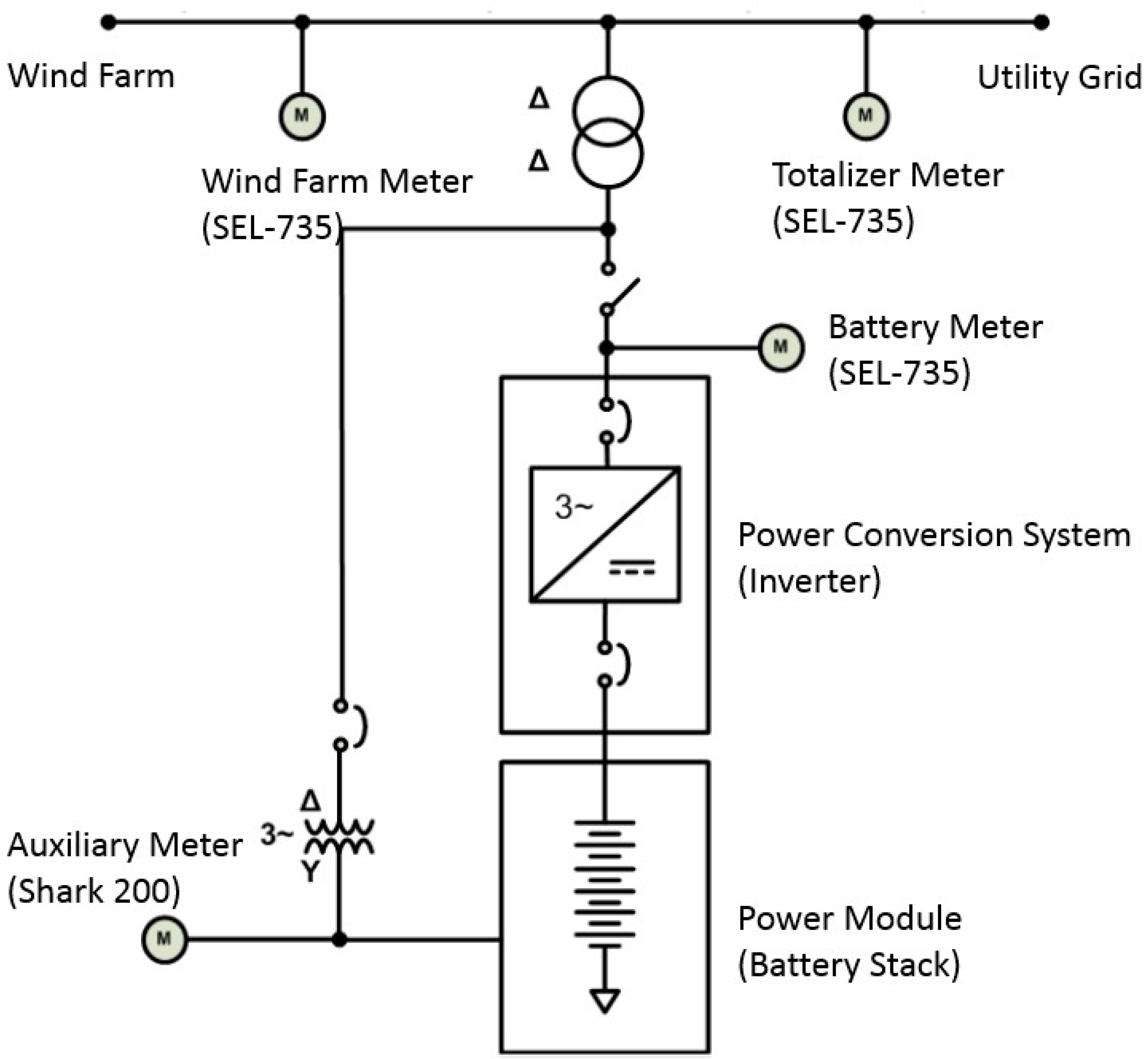
This study was conducted using a 1 MW, 250 kW-Hr lithium-ion titanate BESS that was manufactured by Altairnano Inc. (Anderson, IN, USA). The BESS consists of a power module (a 20,411 kg, 53 ft container housing battery stack) and an inverter (an 8165 kg, 10 ft container). A full description of the BESS is provided in a companion paper [24]. The test site is the electrical grid for the entire island of Hawaii, which has a peak load of about 180 MW and it is currently under penetration by about 32 MW of wind generation. Solar generation on the island is currently around 92 MW. These penetration levels result in significant instantaneous mismatches between generation and load. The BESS is connected to the Hawaii Island electrical grid at the point of common coupling with a 10.6 MW wind farm that is owned and operated by the Hawi Renewable Development (HRD) in the northern region of the island. The interconnection is illustrated in Figure 1. The BESS, which is currently in service, has cycled over 4.25 GW-Hr of energy (8500 equivalent cycles), since its commissioning in December 2012. As part of the agreement with the HELCO, HNEI transferred ownership of the BESS to the utility but retained the right to conduct experiments and access data for research purposes for five years. During this period, HNEI used the BESS to test and optimize control algorithm settings to observe BESS usage (i.e., cycling), as well as its impact on grid frequency.

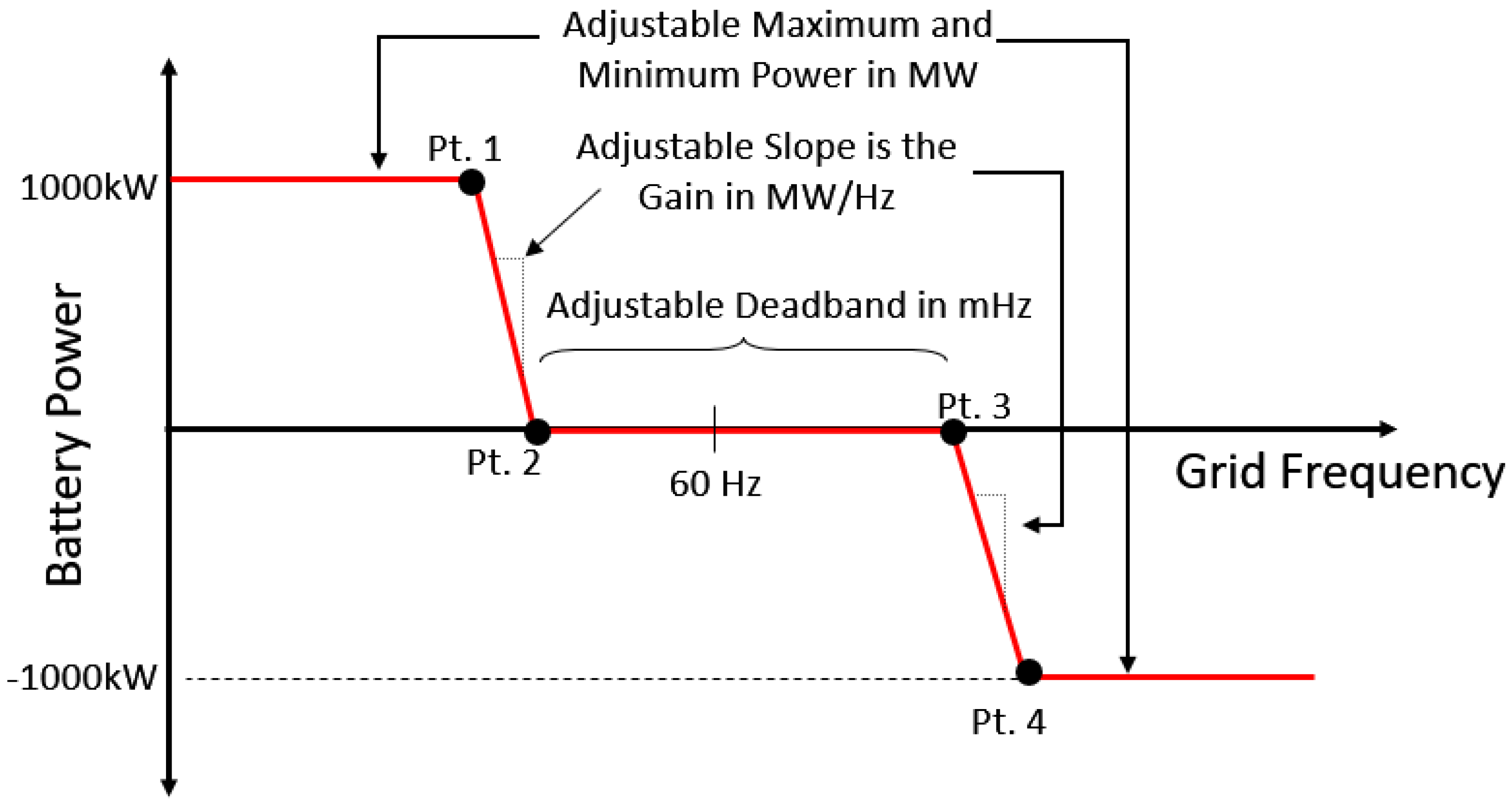
The BESS can be run with either of two control strategies: wind smoothing or primary frequency response. The latter was the focus of this study. The frequency response algorithm was developed around an adjustable frequency-Watt curve (Figure 2) that controls the amount of real power that the BESS delivers to the grid, subject to the operational limits of the BESS, such as the state-of-charge, temperatures of the battery modules, and other limiting factors. The piecewise linear frequency-Watt curve is defined by the values that were assigned to points 1–4. When the power-frequency curve is symmetric, as was the case for this work, the curves are fully defined by the gain and deadband.

• The gain (G) in MW/Hz, is equivalent to the slopes of the lines between Pts. 1 and 2, and Pts. 3 and 4. Gains of 20 MW/Hz and 30 MW/Hz were tested. The original test plan included a gain of 40 MW/Hz, but it was found that the excessive cycling caused the temperature of the battery modules to increase to undesirable levels when this setting was used.
• The deadband (DB) is the magnitude of the frequency change around 60 Hz for which the BESS does not respond to fluctuations in frequency. Deadband widths of 0 mHz, 10 mHz, and 20 mHz were tested (Pt 3 to Pt 2).

Experiments were conducted for each combination of gain and deadband to evaluate the ability to reduce the variability of the grid frequency, while also minimizing energy throughput (i.e., battery cycling). Grid frequency and battery power were measured using two SEL-735 m that were recorded at five times per second. In Figure 1, the real power output (P) of the BESS was measured at the “Battery” meter on the BESS side of the interconnection transformer, and grid frequency (f) was measured at the “Totalizer” meter on the utility side of the interconnection transformer. A gain of 30 MW/Hz and deadband of 0 mHz would be expected to be the most aggressive, with the largest impact on grid frequency and most energy throughput. Similarly, the lower gain of 20 MW/Hz and a deadband of 20 mHz would be expected to be the least aggressive setting, causing the BESS to be least active.

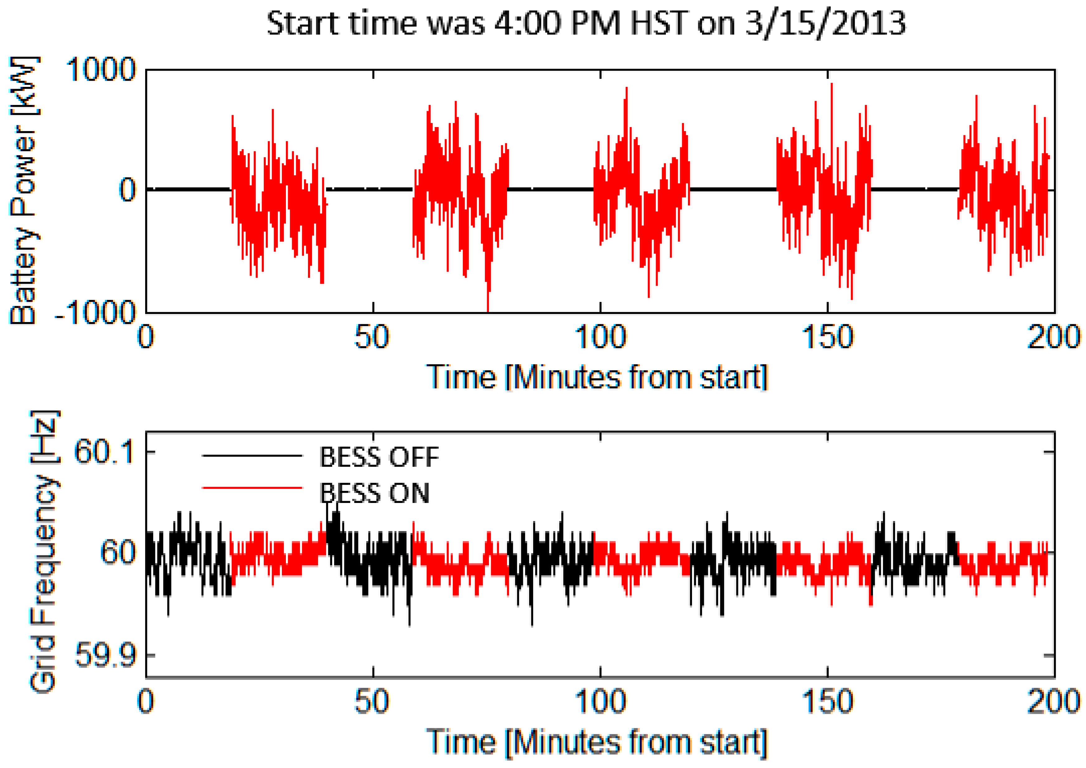
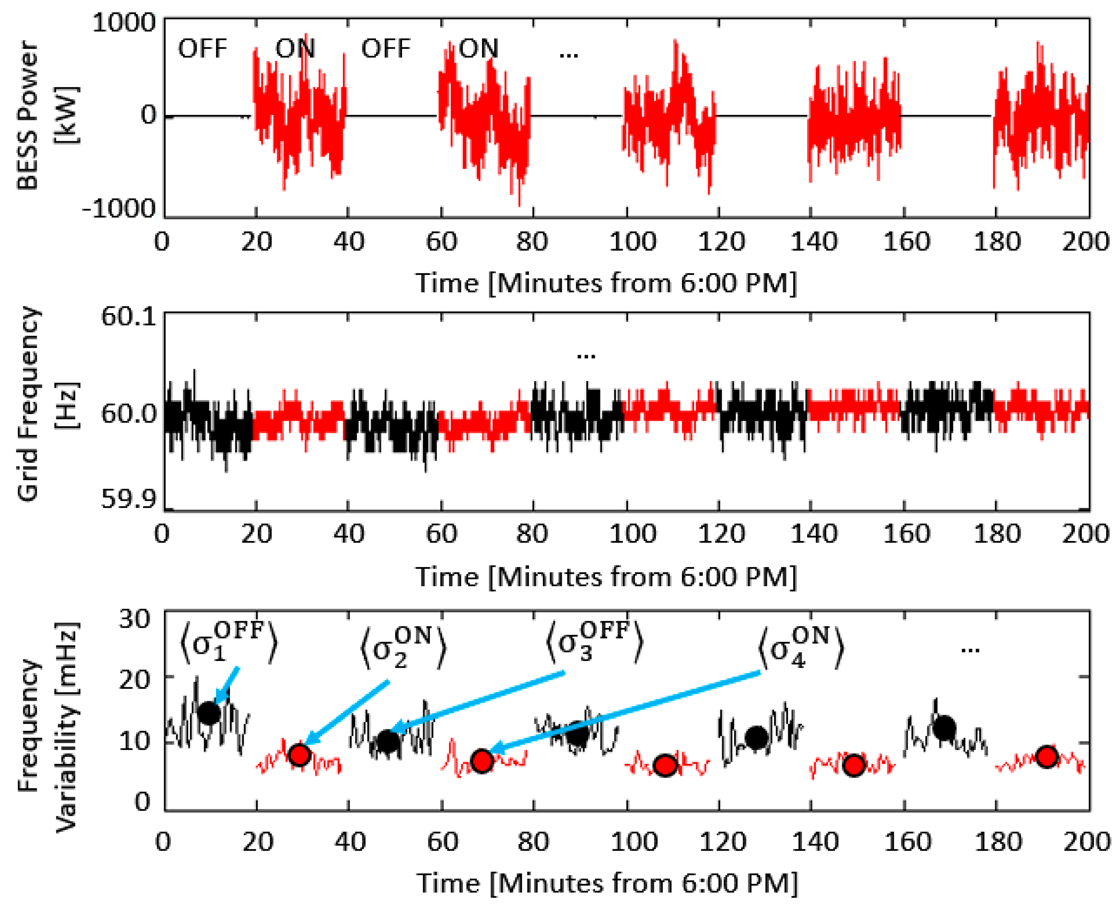
The impact of the BESS was evaluated by comparing grid frequency in consecutive 20-min periods where the BESS was alternated between the inactive (OFF) and active (ON) states. The (top plot in Figure 3 shows P, which goes flat for 20 min at-a-time; this is the toggling between ON and OFF). Various test intervals were considered but preliminary analysis indicated that 20 min provided a good balance between two conflicting requirements: (1) collecting a sufficient amount of data for robust statistical calculations and (2) keeping the test interval short enough that the background grid conditions could be expected to remain relatively constant. Examination of grid frequency variability of both sides of any change in battery status (OFF–ON–OFF, for example) validated the use of a 20-min period. These “switching experiments” with multiple changes between ON and OFF, typically 200 min in duration, were conducted at different times of the day and under different operating conditions (e.g., low wind, high wind, variable wind, etc.). The experiments were conducted in cooperation with HELCO system operators, who were in contact with the HNEI personnel conducting the experiments.

Figure 3 shows the output from one representative 200-min experiment, the top plot shows the real battery power output (P) of the BESS in kW and the bottom plot shows the grid frequency (f) in Hz. Negative P means the BESS is absorbing real power from the grid and positive values mean that the BESS is supplying power to the grid. The periods when the BESS was OFF are displayed in black, and the periods when the BESS was ON are displayed in red.

As described above and discussed in more detail in [24], grid frequency variability was used to quantify the impact of the BESS on the Hawaii grid. It is apparent from a visual inspection of the frequency time series (Figure 3, bottom) that there is a reduction in grid frequency variability whenever the BESS is ON. A reduction in frequency variability was observed in all experiments for all variations of gain and deadband tested.

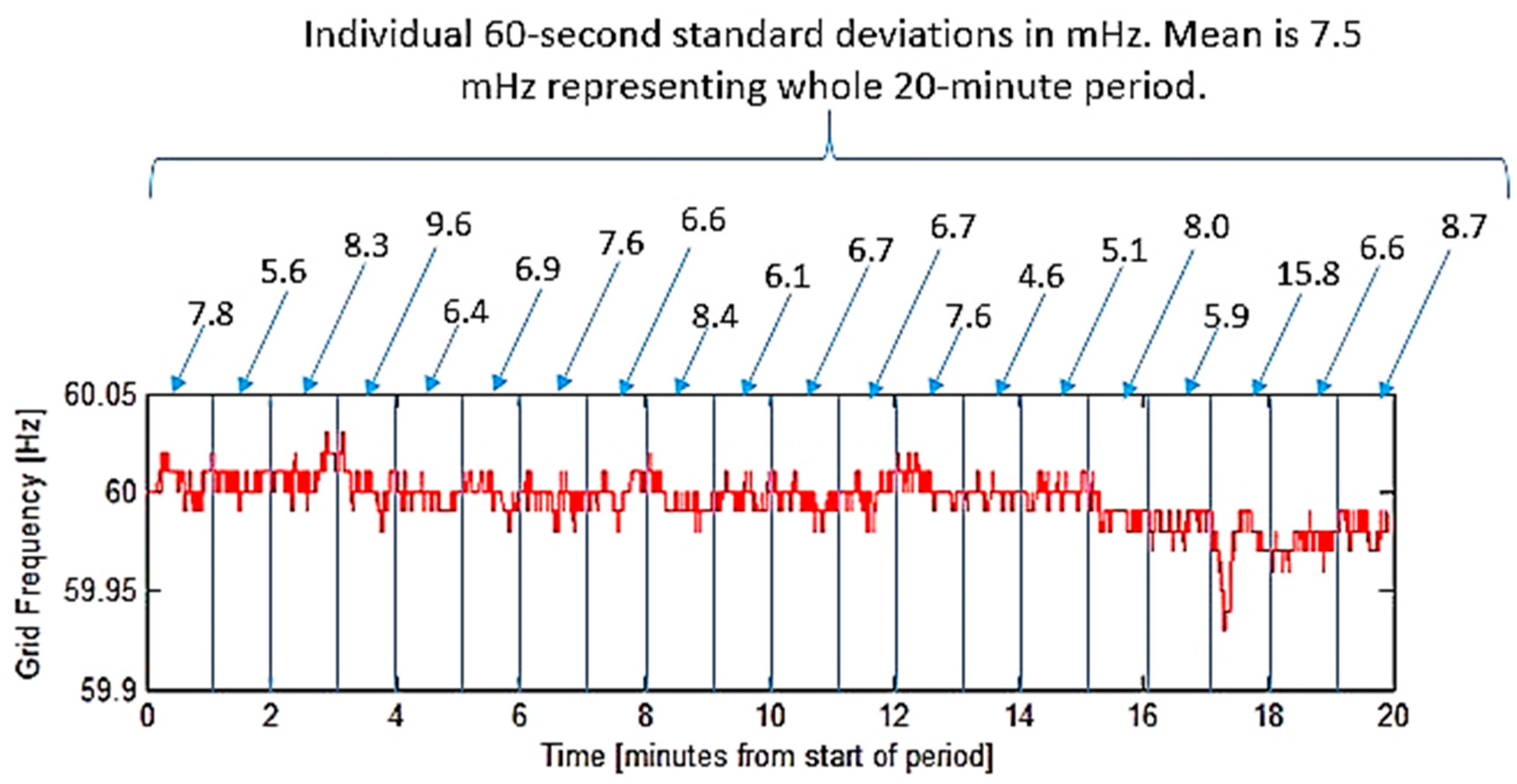
The metric that was used in this study to characterize frequency variability is the standard deviation of the grid frequency over one minute. The rationale for the 60-s timescale was discussed in detail in [24], where it was determined that the relatively short time-scale is needed to characterize the effect of the BESS, as they have a fast response time when compared to HELCO’s diesel generation units.

Figure 4 illustrates the methodology used to determine the frequency variability metric for each 20-min period. The 20-min frequency time series is divided into twenty 1-min windows. The standard deviation of each 1-min window calculated. Then, all 20 are averaged to yield the frequency metric for the 20-min period. The use of 1-min windows averaged over the 20-min periods further reduced the effects from slow variations in grid frequency due to grid operations, which are not of interest when studying a BESS. For notational purposes, the metric of the first period with the BESS OFF is indicated as:

$$<{\mathsf{\sigma }}_1^{\mathrm{OFF}}>,$$

(1)

where the angle brackets (< >) indicate the time mean for the 20-min period, the subscript number indicates the period number (i.e., 1–10 in a single 200-min experiment), and the superscript indicates whether the BESS is ON or OFF.

The comparison of any two consecutive 20-min periods with the BESS on or off allowed for us to determine the impact of the BESS on the grid. Figure 5 (top and middle) shows BESS power and grid frequency for another 200-min experiment where the BESS was alternatively turned on and off. The bottom of Figure 5 shows the calculated frequency variability metric for each 20-min period. Comparing any consecutive 20-min periods shows the expected reduction in frequency variability when the BESS is ON compared to OFF. We will often refer to the OFF periods as “background variability”. This technique not only allowed comparisons over a 200-min experiment, but also allowed comparison across different days and even different grid operating conditions.

In addition to the frequency variability, the total energy throughput of the BESS (kW-Hr) was calculated over each 20-min period that the battery was on.

3. Results

Between 2013 and 2015, eighty-five experiments were performed, each having a duration of 200 min, similar to the one shown in Figure 5. On any single day or night, one 200-min experiment would be conducted with gain and deadband fixed to one of the six combinations that are discussed in Section 2.

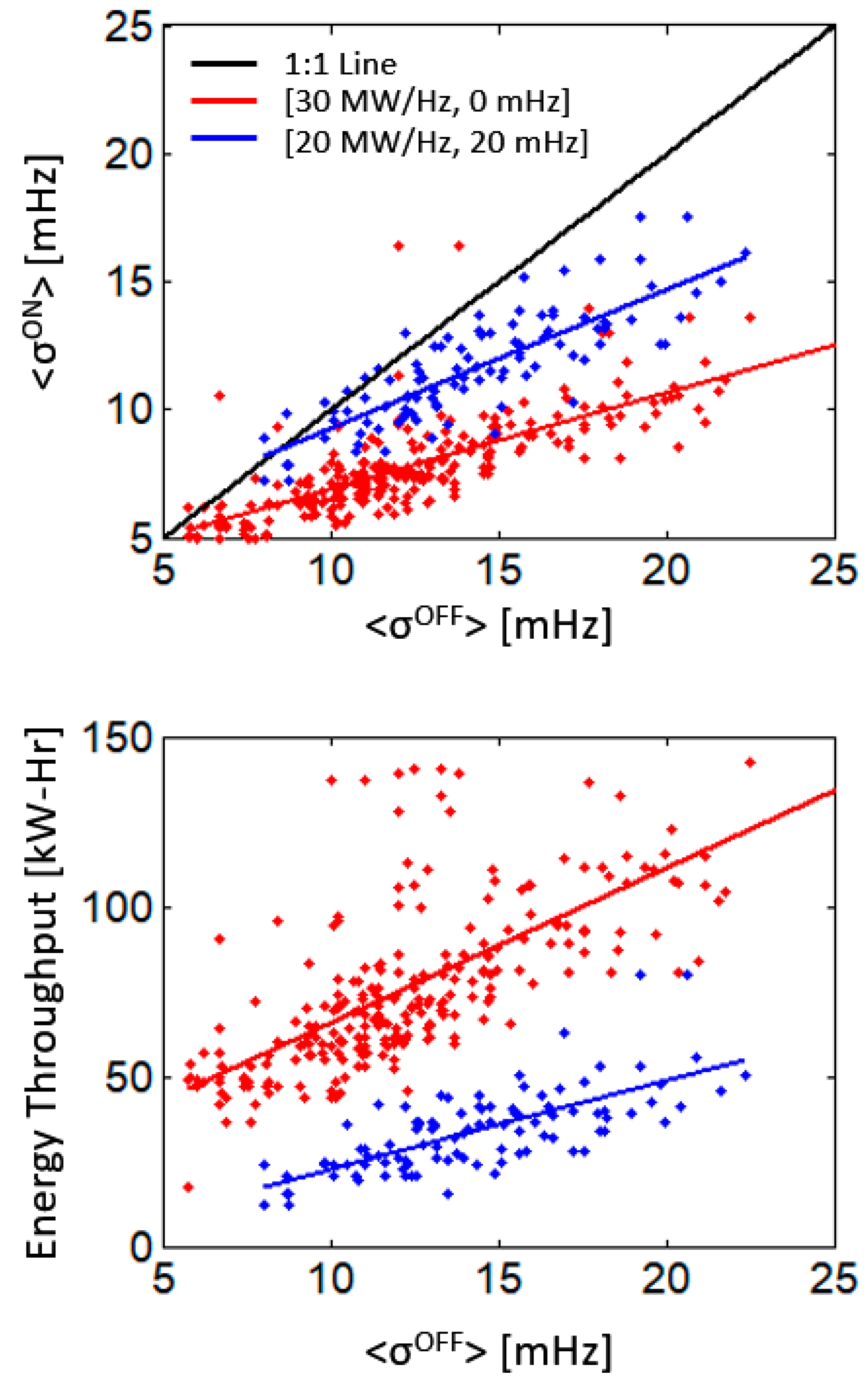
The top plot of Figure 6 displays results from 41 experiments conducted using the most aggressive control parameters (G = 30 MW/Hz, DB = 0 mHz) in red, and the least aggressive (G = 20 MW/Hz, DB = 20 mHz) in blue. The top figure shows frequency variability metric for various consecutive 20-min periods with the battery on versus the battery off. The bottom of Figure 6 shows the energy throughput from periods with the BESS ON, plotted against the background variability metric of the adjacent period with the BESS OFF. Each point (red or blue dots) corresponds to a pair of adjacent 20-min ON/OFF periods.

The black line in the top part of the figure represents the 1-to-1 line, which is equivalent to a frequency variability metric that is equal to the background; that is, no measurable impact of the BESS on grid frequency could be discerned. Any point below the black line represents a reduction in the frequency variability when the battery is on. In Figure 6, the red dots represent the most aggressive control settings while the blue dots are from experiments conducted using the most conservative control settings. The lines represent the least-squares fit for each.

As can be seen in the upper plot of Figure 6, the BESS reduced frequency variability for nearly every pair of ON/OFF periods across the wide range of background grid conditions that were observed during these experiments (forty-one 200-min experiments for the red dots). The best-fit lines indicate that the BESS to is more effective when there is greater background variability (i.e., the percent reduction in frequency variability was greater for the high variability background conditions).

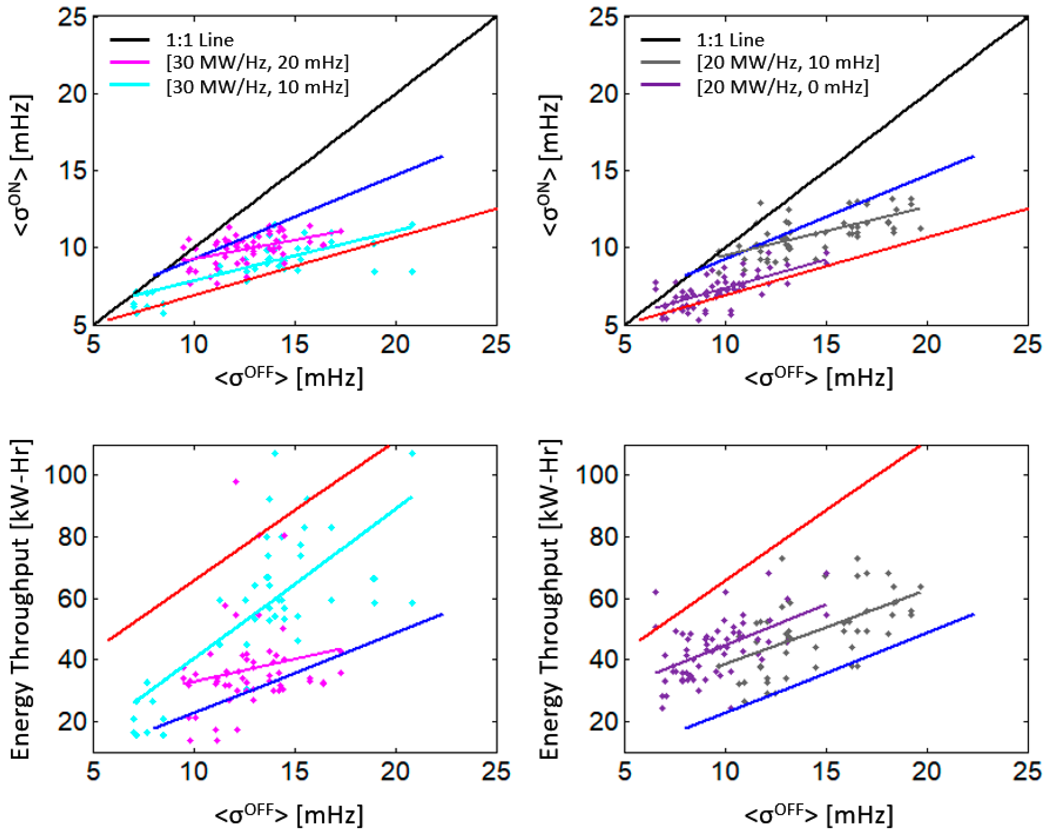
As previously discussed, a total of six combinations of deadband and gain were evaluated. Figure 7 shows the best fit lines from the most aggressive (red) and least aggressive (blue) settings and adds results from the other four intermediate configurations. The plots to the left show experimental results when the gain was 30 MH/Hz with two other deadband settings. The plots on the right show results when the gain was 20 MW/Hz with two other deadband settings.

The frequency variability results that are shown in Figure 7 (top-left and top-right) are within the bounds of the two extreme cases: the most and least aggressive shown as red and blue, respectively. The same is true for the energy throughput measurements (bottom-left and bottom-right). The ideal behavior would be a frequency variability trend-line that approaches the red line (most aggressive case), with an energy throughput trend-line that approaches the blue line (least aggressive).

Some generalizations can be made from the results shown in Figure 7. Higher gain reduces the grid frequency variability, but at the cost of more cycling. Higher gains also reduce frequency variability when the background conditions are less variable, meaning that the BESS action may not have been needed. Larger deadbands reduce cycling when the background variabilities are low, but do not generally reduce frequency variability as well when the grid background variability is high.

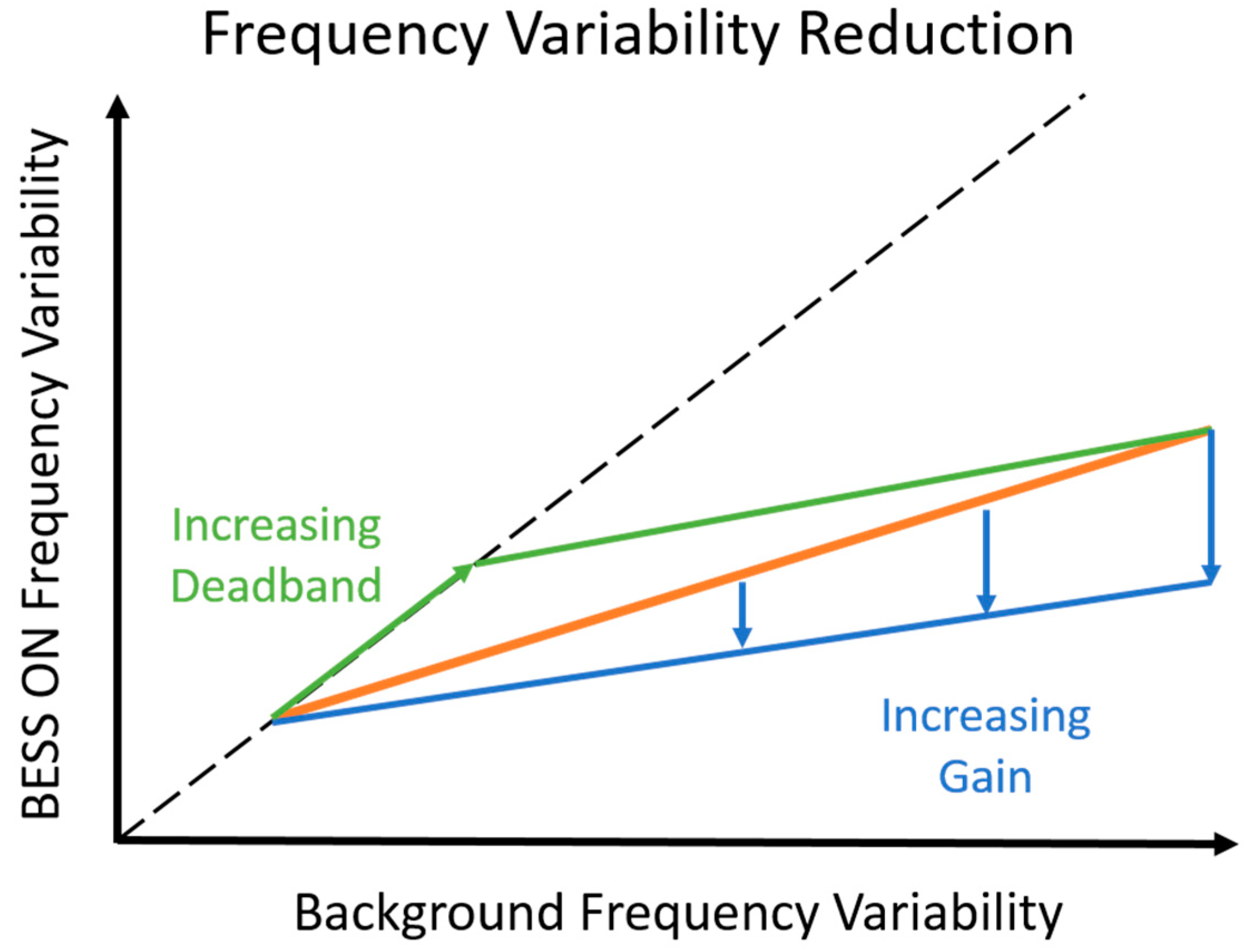
A schematic showing these interactions of the parameter settings is shown in Figure 8. The size of the deadband sets the point at which the BESS responds to frequency variations (green arrow), whereas the gain parameter determines the strength of the BESS response to all frequency excursions above the deadband (blue arrows). At progressively higher frequency variability, the frequency lies outside the influence of the deadband more and more, and the BESS response/effectiveness is increasingly dominated by the gain (blue line).

4. Discussion and Conclusions

In the following discussion, we use the term BESS “Effectiveness”, which we define as the amount that grid frequency variability was reduced with the BESS ON, as compared to an adjacent background variability:

$$\mathrm{Effectiveness}=100·\left(1-\frac{<{\mathsf{\sigma }}^{\mathrm{ON}}>}{<{\mathsf{\sigma }}^{\mathrm{OFF}}>}\right)$$

(2)

The effectiveness of the BESS, based on the best-fit lines in Figure 6 and Figure 7, are shown at the top of

Table 1. Top: The average percent reduction in frequency variability and Bottom: Energy throughput of the BESS under different control algorithm parameter sets and for Low (12 mHz), Medium (16 mHz), and High (20 mHz) background frequency variability regimes. “G” is short-hand for Gain, while “DB” stands for Dead-Band. † and * denote exceptional results that will be discussed further in the following paragraph.

	Low Variability		Medium Variability		High Variability
	Percent Frequency Variability Reduction (Effectiveness)
Percept Frequency Variability	G = 20	G = 30	G = 20	G = 30	G = 20	G = 30
DB = 0	32.4 *	36.1	39.9 *	42.7	44.3 *	46.6
DB = 10	15.9	29.3	29.0	38.9	36.8	44.6
DB = 20	13.7	18.6†	21.7	32.6†	26.4	41.0†
	Energy Throughput (Usage)
Energy Throughput	G = 20	G = 30	G = 20	G = 30	G = 20	G = 30
DB = 0	50.1 *	74.7	60.7 *	93.0	71.3 *	111.3
DB = 10	43.3	50.0	53.0	69.4	62.7	88.9
DB = 20	28.0	35.9†	38.4	41.6†	48.8	47.3†

for three regimes of grid operation, as characterized by the background frequency variability (i.e., with battery off): low (12 mHz), medium (16 mHz), and high (20 mHz). The bottom of Table 1 shows the energy throughput for those three regimes using values from the linear fit lines.

Two of the six configurations are shown in bold (next to symbols) in Table 1 because they show the most effectiveness for relatively low energy throughput requirements. The entries next to the * refer to the (20 MW/Hz, 0 mHz) configuration, which seems to show favorable performance under all background conditions. This setting reduces frequency variability by within 5–10% of the most aggressive (30 MW/Hz, 0 mHz) setting, but requires 33–36% less energy. The entries next to the † refer to the (30 MW/Hz, 20 mHz) setting. Here, the effectiveness is highest for the most variable background conditions. Under those conditions, when compared to the most aggressive settings, we lose only about 12% in effectiveness, but the energy throughput requirement is reduced by about 60%. With this setting, the range of frequency variabilities throughout all conditions is minimized. That is, with the BESS in this configuration, the frequency variability will be similar, regardless of background conditions.

The minimization of frequency variability can be of interest to, say, the developer of an Energy Management System (EMS). Like all expert systems, an EMS performs best when the inputs (frequency) are less noisy (variability), and more predictable (range of variabilities) across different grid operating regimes. This work shows that even a small BESS, optimized for the specific grid conditions, can have a significant impact on frequency variability.

It is important to note that this research was conducted over a span of time when the Hawaii Island grid was evolving (e.g., addition of PV). To mitigate this, we repeated experiments for the six configurations throughout the test period (i.e., 2013 through 2015). In addition, the results shown include data with wind only (night) and with wind plus PV (day).

In this paper, we have presented the impact of different control algorithm parameter sets on grid behavior and have related it to the usage of the BESS, characterized in terms of total energy throughput as opposed to other variables that might relate more directly to battery degradation (e.g., temperature, cycling, or C-rate). While this work was conducted using a li-ion titanate system, the results (battery usage/cycling) are independent of both the battery chemistry and the particular architecture of the BESS, and therefore the most general metric that can be applied to other BESSs. The aging of the lithium-titanate cells that were used in this particular BESS has been presented in other studies [22,23]. Future efforts include more detailed characterization of individual battery packs for better prediction of the lifetime of the system.

Frequency variability was the topic of this paper. However, large frequency events that occur often on a small island grid are also an important topic of interest. Work is currently underway assessing the impact of a modified frequency response control algorithm for large events on the island of Molokai.