Risk Data Analysis Based Anomaly Detection of Ship Information System


College of Engineering Science and Technology, Shanghai Ocean University, Shanghai 201306, China
*
Author to whom correspondence should be addressed.
†
These authors contributed equally to this work.
Energies 2018, 11(12), 3403; https://doi.org/10.3390/en11123403
Submission received: 1 October 2018
/
Revised: 23 November 2018
/
Accepted: 25 November 2018
/
Published: 4 December 2018
(This article belongs to the Special Issue Selected Papers from EEEIC 2018—18th International Conference on Environment and Electrical Engineering)
Abstract
:Due to the vulnerability and high risk of the ship environment, the Ship Information System (SIS) should provide 24 hours of uninterrupted protection against network attacks. Therefore, the corresponding intrusion detection mechanism is proposed for this situation. Based on the collaborative control structure of SIS, this paper proposes an anomaly detection pattern based on risk data analysis. An intrusion detection method based on the critical state is proposed, and the corresponding analysis algorithm is given. In the Industrial State Modeling Language (ISML), risk data are determined by all relevant data, even in different subsystems. In order to verify the attack recognition effect of the intrusion detection mechanism, this paper takes the course/roll collaborative control task as an example to carry out simulation verification of the effectiveness of the intrusion detection mechanism.
1. Introduction
With the constant intellectualization of industrial equipment, the working performance of a Supervisory Control And Data Acquisition (SCADA) system turns out to be highly dependent on the accuracy and security of communication among the units in closed-loops [1]. However, such systems are normally intricate and fragile, and several striking examples have confirmed that even well-protected SCADA systems can be ultimately crashed [2,3,4,5,6]. Therefore, the cyber-physical security of SCADA systems will be more and more important [7], which has been described by IEEE: “In contrast to cyber security, the goal of cyber-physical security is to protect the whole cyber-physical system, which uses widespread sensing, communication and control to operate safely and reliably.” [8]. Normally, according to the different focus points, the study of cyber-physical security can be divided into defense [9,10], detection [11,12], and maintenance(including repair, reconstitution, etc.) [3,13,14]. Here, we mainly focus on the anomaly detection topic in the cyber-physical security of SCADA. Actually, several effective anomaly detection methods have already been proposed in the anomaly detection area such as system modeling [15,16,17,18,19,20] and data-based analysis [20,21,22,23,24,25], which should always accept a compromise in the modeling uncertainty and data complexity. Besides model-based and coupled data-based intrusion detection, some intrinsic properties of SCADA are considered in detection. In [26], a methodology that uses information extracted from Radio Frequency (RF) features to identify changes was proposed. Meanwhile, S.-M.Jung and J.-G. Song et al.presented an idle-time measurement system in data spoofing detection [27]. Actually, these solutions bring a new perspective to anomaly detection, and the applications for these theories are restricted more or less, which cannot be overcome. However, in [28], an innovative approach based on the concept of critical state analysis and state proximity was presented: attacks can be detected by a set of critical rules, which are formulated in the Industrial State Modeling Language (ISML). Such rules are based on all related data that are not confined to the coupled data. Therefore, the anomaly detection mode we propose in this paper is based on the risk data, which are obtained by the analysis of critical data.
2. Model Description
As a typical SCADA system, the Ship Information System (SIS) is widely used in the connection between each ship electronic system, which are spread across the whole ship. As the data in SIS are designed to be closed and inflexible, firewall updating and off-line detection are difficult to implement. Furthermore, for a ship on a long voyage, any physical or informational damage may cause an irreparable breakdown, which leads to a helpless situation.
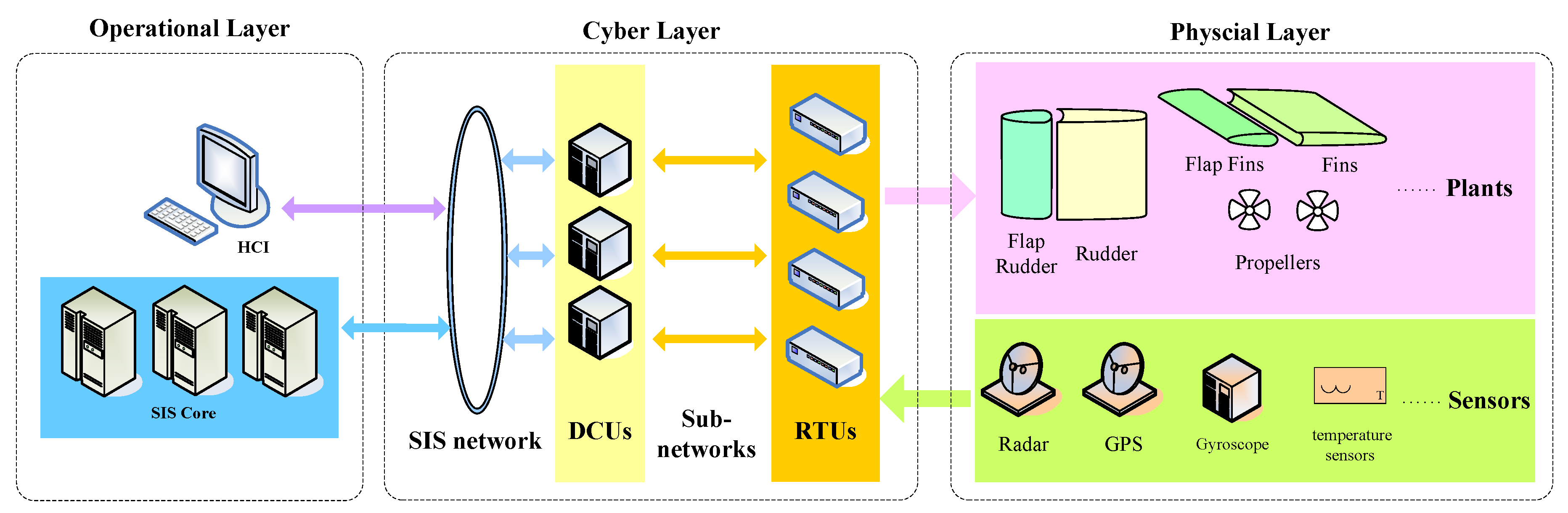
Although different ships have different functions [29,30,31,32,33,34,35], all definitions found in the literature for SIS have one key feature in common. As shown in Figure 1, this defining feature is that SIS is composed of several independent subnetworks and a total ship communication network, which can exchange information (reference input, plant output, control input, etc.) among subnetworks and systems. The architecture of SIS is similar to each normal SCADA, which is listed in the following.
2.1. Structure
2.1.1. Components
Operational Units
Due to the different command types of the mission and situation, a supervisory control command can be released by a user through the Human Computer Interface (HCI) or SIS core. The SIS core provides a common environment hosting the majority of the ship’s applications on a redundant infrastructure, whose targeted hardware location is designed to be transparent to the applications. Some basic control commands are released by the core automatically and spontaneously, such as fire detection, anti-rolling control, etc. Meanwhile, real-time assistant decision support is also done by the core and submitted to HCI.
Distributed Controller Units
The Distributed Controller Units (DCUs) in SIS are networked and interfaced with the SIS network; their duty is to monitor and control every closed-loop system in the ship by coding predefined sequences and control algorithms.
Remote Terminal Units
The Remote Terminal Units (RTUs) in SIS serve as the interface point to DCUs and a variety of analog and digital sensors and actuators. Every RTU is connected with its closest DCU. The telemetry hardware structure of RTU has the capability of sending digital sensor data to the DCU and receiving digital commands from it.
It should be mentioned that, in order to keep the security and anti-damage capability of SIS, each RTU is connected to two DCUs simultaneously, but only one is activated during the running process; such a dual-station structure is widely used in SCADA. For each , its backup DCU is denoted as .
2.1.2. Networks
SIS Network
As a backbone network of the ship information system, the fundamental layering rule of the SIS network is to add maximum DCUs in the ship environment, which leads to a dual-ring network being chosen in the design of the SIS network. Every DCU is led into the SIS network proximally.
Subnetworks
As introduced in [35], numerous DCUs are connected in the SIS network; meanwhile, each of them has the responsibility for dozens of RTUs, which constitute an underlying subnetwork.
Due to the limited space, more design details and examples of implementations can be seen in [29,36].
For SIS, due to different emphases, there exist two structures of SIS, which are the cooperative control structure () and the hierarchical task structure (). is used to describe the implementation method of task control in SIS, while is for the description of task capabilities.
2.2. Cooperative Control Structure of SIS
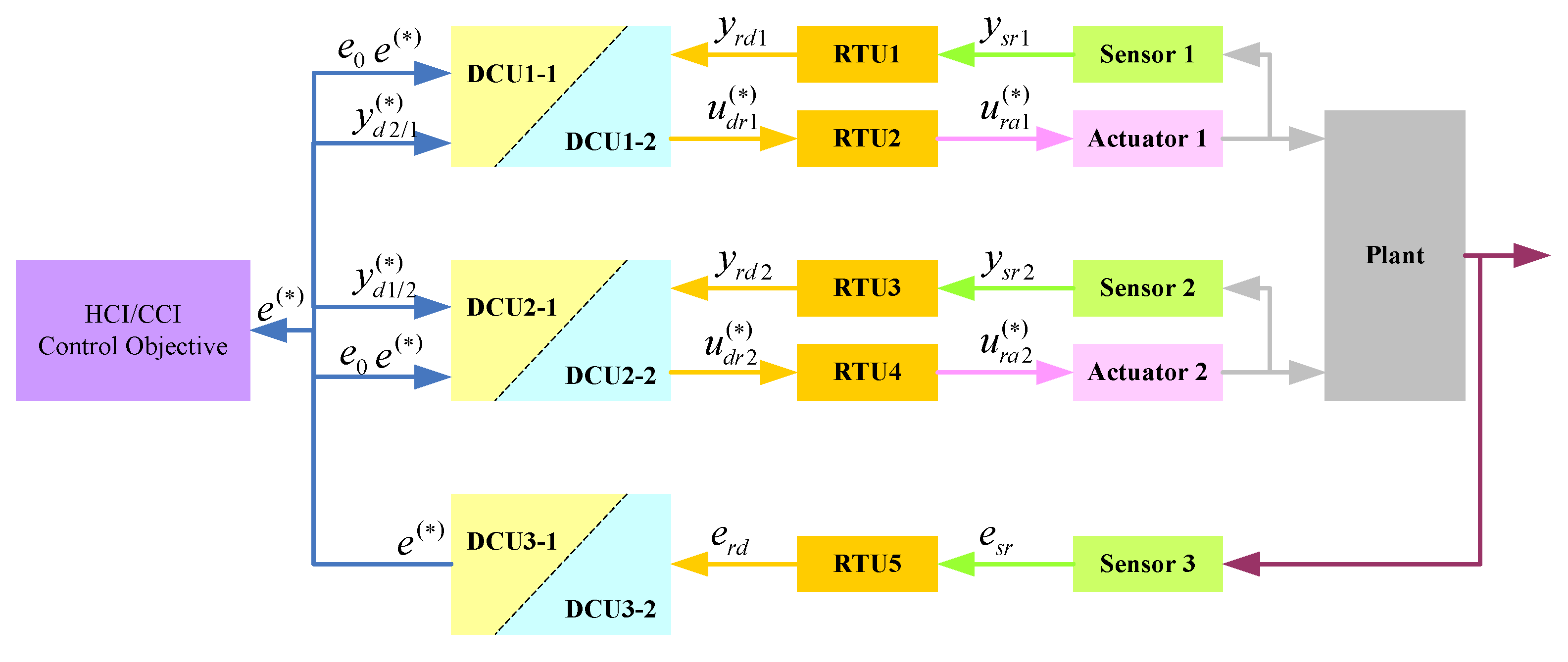
As the connection principle between DCU and RTU is mere proximity instead of task relation, which has reduced the difficulty of planning and laying out networks greatly, but has increased the complexity of every control process in SIS, most missions in SIS are designed to be completed by several DCUs cooperatively. For definiteness and without loss of generality, the cooperative control mode of SIS is shown in Figure 2.
As our attention in this paper is the cybersecurity issue in SCADA, to facilitate distinction, all the data in different lines are relabeled, as is listed in Table 1.
The control objective should be performed by Actuator 1 and Actuator 2 cooperatively. is the control feedback of the control objective at step k, and these data are sampled by a global sensor, Sensor 3. Here, Sensor 1 and Sensor 2 are regarded as local sensors, which are used to sample the running conditions of Actuator 1 and Actuator 2, respectively, and these data are finally received by DCU2-1(2)and DCU1-1(2). Taking DCU1-1 as an example, due to the cooperative structure with the coupling relationship with DCU2-1(2), the control output is determined by the preset distributed control algorithm based on e, , and . As shown in Table 1, if the data are related to a backup DCU, they would be marked with superscript “”, such as , , , etc.
In this paper, taking DCU1 for example, we propose a cooperative state space control model, which is established in Equations (1) and (2).
where is the quantity of state and and are the obtained output for Actuator 1 and 2 from numerical calculation, respectively. As DCU 1 only focuses on the control of Actuator 1, has no physical application, but is only used in the revision of obtained by amending function . Meanwhile, the communication access of at step k is denoted as and . As the communication between DCU and RTU belongs to a kind of multi-channel real-time mechanism, the access is granted constantly. However, the communication among DCUs and the HCI/CCIcore should follow an access specification. For example, if DCU1-1 gains access to publish data at step k, we have:
Equation (1) provides a new model to analyze the control progress of cooperative control mode based on data, and the control output of one actuator would be corrected by the execution conditions of its collaborators. can be determined by a neural network, fuzzy, or linear regression algorithm, etc, and as a representative example in [37], we propose a variable universe fuzzy algorithm to correct the deviation between two cooperative rudders.
As our research interest in this paper is cybersecurity, the transmission process of a data is worth more serious study than its solution process. The optimization of will be researched in the future; in this paper, we assume that each DCU in the cooperative control mode would figure out a suitable control output for the corresponding actuator, giving sufficient thought about its collaborators.
3. Signal Attack in SIS
Due to the structure analysis above, two types of attacks are proposed and researched in this paper, which are Signal Attack and Mode Attack . Ultimately, the core objective of all the attacks intruded in a SIS is to cause a risk. For an , it has the ability to modify a regular signal into a dangerous one, while can create a risky task. In this paper, our attention is mainly focused on .
3.1. Signal Attack Form
It should be mentioned that there are some differences between the signal attack and jamming attack. The signal attack can modify the content of the data flow, but keep the format and reachability. The data flow would be blocked by the jamming attack.
Equation (4) is a typical form of , which has the ability to denote almost all of inside attacks existing in SCADA except the Denial of Service (DoS) attack.
where is a set of input data , , is the output of modified by the attack at step k, and is a threshold of max(min)variation between and . The subscript is the label of the device (including DCUs and RTUs), which is planned to handle .
It should be mentioned briefly that the DoS attack on a controlled closed-loop in SCADA is an attempt to make the network resource unavailable, against its requirements of reachability and observability. Based on the research results, we proposed in [38,39] that if a DCU has sent -data in one data flow by to keep the closed-loop system -step observable, is considered to be attacked on , if for each where , we have . That means the DoS attack has the ability to modify the DCU’s predefined sequences. A DoS attack on can be detected by a related or CCI, intuitively, if they fail to receive scheduled and planned data from .
3.1.1. An Example of the Signal Attack Algorithm
Based on the definition of the signal attack, an example of the insertion attack algorithm is given in Algorithm 1, which operates as follows.
| Algorithm 1 Signal attack algorithm. |
| Require: Original input data |
| 1: remark ; |
| 2: initialize ; |
| 3: ; |
| 4: for to n do |
| 5: ; |
| 6: end for |
| 7: ; |
| 8: ; |
| 9: if then |
| 10: ; |
| 11: ; |
| 12: else |
| 13: ; |
| 14: ; |
| 15: end if; |
| 16: ; |
| 17: ; |
| 18: ; |
| 19: for to 1 do |
| 20: ; |
| 21: end for |
| 22: ; |
| 23: return ; |
It takes as input original input data . Line 1 of the algorithm denotes each element in set as . After that, a set is initialized in Line 2 to store the variation between each and (Lines 4–6). Basic modified data are stated by choosing data in (Lines 7–8) randomly. Here, is a typical way to select a uniformly-distributed random number, which is from the range by using the MWCalgorithm. In addition, from Lines 9–16, a further modification is executed to confuse the IDSaimed at replay attack. The addition value denoted as r is based on the maximum or minimum of , which is determined by the numerical relationship between and . Lines 11 and 14 can keep r from the IDS based on data. What is more, the detection by the threshold would also be invalid by the restraint in Line 18. The output of the insertion attack algorithm is given in Line 23.
3.1.2. The Form of the Hazard Factor-Based Signal Attack
According to the form of the basic signal attack, in order to find the balance between the hazard and invisibility requirements of signal attack, a new type of signal attack is presented in this paper. This has an additional parameter named hazard factor (denoted as ). For the given original data signal and the corresponding typical signal attack , we have:
where is the output of the hazard factor-based signal attack. According to the different values of , can be further classified as:
; if we have , the signal attack does not exist;
is the lower hazard, if ;
is equivalent to , if;
would be the higher hazard, if , and here, is the maximum allowed hazard factor of , which can be hidden from the IDS.
3.1.3. Signal Attack Zone
As shown in Figure 2, according to the refined model of SIS, there exist several point-to-point communication lines that make up a closed-loop system. The insertion attack may happen in any node between two lines. Here, we defined each probable attack zone in a cooperative SCADA, which are listed as follows.
Attack on Local Sensor Data
A local sensor is used to sample the running status of one actuator, which is activated by the cooperative control mission. Normally, for local sensor data (Sensor 1 as an example), without being attacked, we have . Such data may be attacked on RTU1, which leads to or if DCU1-1(2) is attacked.
Attack on Global Sensor Data
As shown in Figure 2, for the global Sensor 3, in an ideal case, we have . An insertion attack may tamper with the data as a result of or if the attack is embedded in RTU3 or DCU3-1(2).
Attack on Actuator Control Data
Finally, an actuator also can be attacked in SCADA by causing an undetected misoperation in RTU2. Meanwhile, if the calculational result of the control algorithm in DCU1-1(1) is attacked, would be an incorrect output, which means , where is denoted as the calculational result.
4. Critical State Analysis
4.1. Critical State Estimation
In this paper, the Critical State Estimation (CSE) algorithm we propose is based on the Industrial State Modeling Language (ISML), which was first proposed by A. Carcano et al. in [28]. The rules in the ISML are formulized as where is a Boolean formula composed of several predicates, which are used to indicate the values that are assumed by critical components. The definition of ISML is listed in the following.
where is a register; Discrete Input, Coli, Input Register, and Holding Register are denoted as , respectively. The ISML is used to describe a particular class of system states called critical states that correspond to dangerous or unwanted situations in SIS. Here, the risk level of each state is reversed by its confidence. The risk level is considered to be in the critical state, where a value of one means low risk, while five is a surely dangerous critical state of SIS. Here, denotes one kind of data in SIS, and means the critical state value () of when the risk level reaches by , for example if such a rule is set in SIS:
We have , which means for , the critical state value is >2500 (with risk of ), when its related data .
Therefore, the anomaly detection and critical state estimation algorithm is given in Algorithm 2, which operates as follows.
| Algorithm 2 Critical state estimation algorithm. |
| Require:, ( level of ), -related rule set , -related dataset |
| 1: reorder and remark ; |
| 2: for to 5 do |
| 3: for to do |
| 4: Initialize interval |
| 5: remark the -related subset of as ; |
| 6: Set subinterval |
| 7: |
| 8: |
| 9: Set interval |
| 10: |
| 11: |
| 12: if then |
| 13: ; |
| 14: end if; |
| 15: if then |
| 16: ; |
| 17: end if; |
| 18: if then |
| 19: ; |
| 20: end if; |
| 21: if then |
| 22: ; |
| 23: end if; |
| 24: end for |
| 25: if or then |
| 26: is beyond p-level risk; |
| 27: else |
| 28: is p-level non-risk; |
| 29: end if; |
| 30: end for |
| 31: return and |
It takes as input original input data , where the physical meaning of is determined by its ; meanwhile, the -related rule set is needed, as well. According to , all related are necessary and stored in dataset . It should be mentioned that is not equivalent to the set of all coupling data. Line 1 of the algorithm restores each rule of by its risk level and denotes these rules as where p is the risk level. Lines 2–30 show the critical state estimation method, for each rule and its related dataset ; a critical state of is determined. Line 6 creates a safe subinterval for under rule , and the interval is shrunk during each loop computation in Line 9. Lines 10–11 show the upper and lower bound of , denoted as and , respectively. Lines 12–23 show the way to find the determinant factors (denoted as and ), which leads to being risk data or not. Lines 25–29 shows the anomaly detection method, if , is the p level risk of non-arrival or it is called beyond the p level risk. Due to the different importance of each , its Risk Tolerance is different. For four-level data , if the judgment result is beyond four levels of risk, is anomalous data. Line 31 returns all upper and lower bounds of each risk level for , which is . Meanwhile, the the determinant factors (denoted as and ) are uploaded, as well.
4.2. Bi-Critical Data Analysis
According to Algorithm 2, such data, the value of which is beyond the critical state, are determined; however, there exists the possibility that one normal datum is miscalculated, caused by a related datum, which is actually anomalous. Here, we propose the definition of bi-critical data to identify the true abnormal data from two related data.
Definition 1 (Bi-critical Data ): Two critical data , data , and , data , in SIS are regarded as a pair of , if or .
According to Definition 1, a further analysis of critical state discrimination is proposed in Algorithm 3. Here, we assume that .
| Algorithm 3 Critical data discrimination algorithm for a pair of . |
| Require:, , , , -related rule set , -related dataset initialize a -related dataset , which includes every type of data belong to , except initialize a -related, but non-related rule set choose , , , as inputs, and run Algorithm 2 if the result of Algorithm 2 shows that is beyond -level risk then return is a definitely beyond -level risk () else reset choose , , , as inputs, and rerun Algorithm 2 if the result of Algorithm 2 shows that is beyond -level risk data then return is definitely beyond -level risk data () else return is potentially beyond -level risk data () end if end if |
Here, in Algorithm 3, we propose a two-layer discrimination mode. It takes as input original input data , , , -related rule set , and -related dataset . In Lines 2–3, two subsets of and , which exclude the factor of , are denoted as and , respectively. In Line 4, Algorithm 2 is called to calculate the critical data situation of without considering the existence of . If the result shows that is still a beyond -level risk, that means is Definitely Risk Data () whatever the value of . If is a -level non-risk by the analysis based on Algorithm 2, further discrimination is presented in Lines 7–13. As the data sampling mode of SIS is based on the zero-order holder (ZOH), here we treat as unadopted data and reset ’s value at step k as . Then, Algorithm 2 is called again at Line 8. If is still a -level risk, it means is a , while is a core determinant of ’s riskiness. If is not a -level risk according to the modified result of , such a possibility should exist that is non-risk data, but it should be marked in a miscalculation caused by the risk data . Due to the nondeterminacy of risk level, this kind of is named as Potentially Beyond -level risk Data (). In this paper, due to the uncertainty of the risk level, a issue in SIS would be considered as a higher priority than a .
5. Simulation
5.1. Modeling of the Ship Cooperative Motion Control System
Due to the complexity of ship motion, it has six Degrees Of Freedom (DOF) as a general rule, which can be described as u (surge velocity), v (sway velocity), w (heave velocity), r (yaw rate), p (rolling rate), and q (pitching rate). In this paper, we mainly focus on three motions: ship surging, ship heading, and ship rolling, and the ship motion model we chose in this paper is in Equation (7).
where m is the mass of the ship and , , are respectively denoted as the rolling, pitching, and yawing angular acceleration. is the coordinates of the position vector about the center of the ship’s gravity in the moving coordinate system. , , and are respectively denoted as the longitudinal force, heading resultant moment, and rolling resultant moment. J is the inertia matrix of the ship, when the origin of the coordinate system is not the center of the ship’s gravity, as Equation (8) shows.
As the system is constituted by two rudders, two propellers, and a pair of fins, the compositions of ,, and are shown in Equation (9):
where are respectively denoted as fluid inertia, fluid viscosity, right propeller, left propeller, right rudder, left rudder, fins, and disturbances. As is shown, every plant working in the system has the ability to change the ship’s surging, heading, and rolling more or less, which depends on the moment it produced in different DOF. This behavior increases the importance of cooperative control algorithms, which means we also need a real-time communication environment.
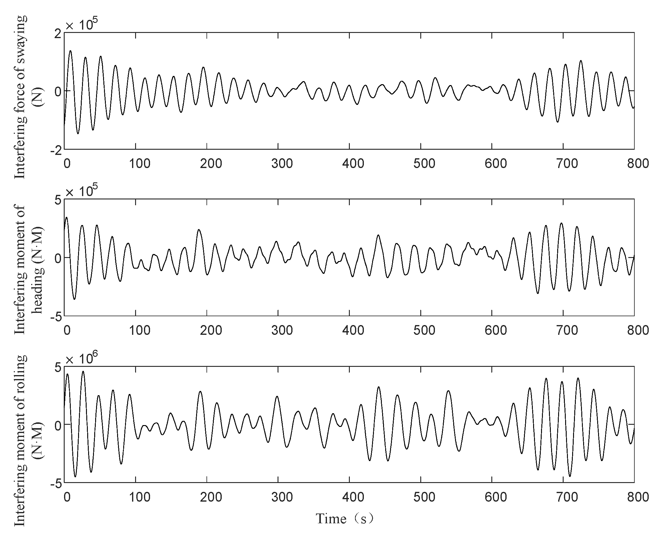
Of many possible external disturbances acting on the ship motion process, the waves are the most important external disturbances and dominantly influence the control performance. As the wave disturbance can be treated as a typical stationary random process satisfying a Gaussian distribution, the spectrum of the random ocean wave is given in Equation (10):
where P-Mspectrum is chosen as the initial spectrum, V is the ship speed, and is the wave angle.
Therefore, the interfering moment of wave disturbance can be determined as:
where , , , is the amplitude of each harmonic, M is the number of energy partitions, is the beam, L is the length, and is the average draft.
In this paper, the ship chosen in the simulation has a displacement of 2500 tons, and we have , , .
According to the wave disturbance model above, in such conditions in which significant wave height is four meters and the wave angle is , the force and moment of sea wave disturbance are shown in Figure 3.
5.2. Influence of Signal Attack in SCMCS
Under the simulation results of ship dynamics, in this subsection, the influence of signal attack in the Ship Cooperative Motion Control System (SCMCS) is researched and analyzed. In order to establish the closed loop, the distributed collaborative control algorithm of ship heading and rolling we adopt here is based on a PID-fuzzy fusion control law, which was proposed in [40]. This fuzzy PID fusion controller was designed through continuous updating of its output scaling factor. Instead of using a unitary fuzzy or PID algorithm, the fusion weighted summation rule bases are used in parallel, which improved the performance of the proposed fuzzy PID controllers compared to others. The fusion FPID parameter is calculated as:
where is the output by each control algorithm (the fuzzy controller and PID controller are treated as subprograms of the fusion algorithm), is the fusion factor of each subprograms, and n is the number of total subprograms in a fusion algorithm; normally, there are . In this paper, the fusion factor is chosen as:
Due to the space limitation, the working principle and application effect of this algorithm will not be introduced in this paper. The simulation results of ship heading and rolling based on this control algorithm are shown by dotted lines in Figure 5A,B, respectively. Meanwhile the solid line in Figure 5A,B depicts the heading and rolling output of the ship while the signal attack acted on the heading data signal. Here, the signal attack first happened at 80 seconds, and we have . In addition, the operation states of main (flap) rudder and main (flap) fin are shown by solid (dotted) lines in Figure 5C,D, respectively. Due to the coupling relationship between ship heading and rolling, the manipulation of heading sensor data can also change the effect of the rolling control system, and the mathematical statistics results are listed in Table 2.
5.3. Anomaly Detection Analysis of SCMCS
In this paper, based on the running effect in the semi-physical simulation platform, which was introduced in [36], the risk data rule is set as follows:
The notations of each rule are listed in Table 3.
Here, we assume that the Risk Tolerance of SCMCS in SIS is 4, which means only Rule 1, 2, 5, 6, 8, 9 and 10 need to be taken into account. And these rules are used to limit the data in and . As shown in in Figure 6, according to Algorithm 3, the abnormal data of ship rudder and flap rudder are first detected at 81.7 s and 80.4 s, respectively.
6. Discussions and Conclusions
In this paper, the basic structure of the ship information system and its typical cooperative control mode were formulated. According to such structure, a signal attack detection method was proposed. Under the consideration of coupling data flow, we improved the Critical State Estimation (CSE) algorithm proposed in [28] by setting new sentence patterns of the Industrial State Modeling Language (ISML). Therefore, such risk data can be determined by the related data and a set of predefined rules. The simulation result shows that wherever the data are attacked by the signal attack in the cooperative control loop, this can always be detected. We have to point out that we did not focus on the prevention of signal attack in the paper. For now, waking up a related spare DCU is the typical reconstitution strategy when the signal attack is detected. More intelligent solutions can be researched in the future.
Author Contributions
B.X. conceived of and designed the experiments; S.C. performed the experiments; Y.J. and Y.L. analyzed the data; S.C. contributed analysis tools; B.X. wrote the paper.
Funding
This paper is sponsored by the Shanghai Sailing Program (No. 18YF1409900) and the Shanghai Innovation Action Plan (No. 17050502000).
Conflicts of Interest
The authors declare no conflict of interest.
References
- Mo, Y.; Kim, H.J.; Brancik, K.; Dickinson, D.; Lee, H.; Perrig, A.; Sinopoli, B. Cyber–Physical Security of a Smart Grid Infrastructure. Proc. IEEE 2011, 100, 195–209. [Google Scholar]
- Slay, J.; Miller, M. Lessons Learned from the Maroochy Water Breach. Int. Fed. Inf. Process. 2007, 253, 73–82. [Google Scholar]
- Abrams, M.D. Malicious Control System Cyber Security Attack Case Study–Maroochy Water Services, Australia. In Proceedings of the Annual Computer Security Applications Conference, Anaheim, CA, USA, 8–12 December 2008; Volume 253, pp. 73–82. [Google Scholar]
- Nicholson, A.; Webber, S.; Dyer, S.; Patel, T.; Janicke, H. SCADA security in the light of Cyber-Warfare. Comput. Secur. 2012, 31, 418–436. [Google Scholar] [CrossRef]
- Langner, R. Stuxnet: Dissecting a Cyberwarfare Weapon. IEEE Secur. Priv. 2011, 9, 49–51. [Google Scholar] [CrossRef]
- Ten, C.W.; Liu, C.C.; Manimaran, G. Vulnerability Assessment of Cyber Security for SCADA Systems. IEEE Trans. Power Syst. 2008, 23, 1836–1846. [Google Scholar] [CrossRef]
- Knijff, R.M.V.D. Control Systems/SCADA Forensics, What’s the Difference? Digit. Investig. 2014, 11, 160–174. [Google Scholar] [CrossRef]
- Nate Kube.Cyberphysical Security: The Next Frontier. Available online: http://www.securityweek.com/cyberphysical-security- next-frontier (accessed on 23 March 2015).
- Pollet, J. Developing a solid SCADA security strategy. In Proceedings of the 2nd ISA/IEEE Sensors for Industry Conference, Houston, TX, USA, 19–21 November 2002; pp. 148–156. [Google Scholar]
- Ten, C.W.; Manimaran, G.; Liu, C.C. Cybersecurity for Critical Infrastructures: Attack and Defense Modeling. IEEE Trans. Syst. Man. Cybern. Part A. Syst. Hum. 2010, 40, 853–865. [Google Scholar] [CrossRef] [Green Version]
- Barbosa, R.R.R.; Pras, A. Intrusion Detection in SCADA Networks. In Mechanisms for Autonomous Management of Networks and Services; Springer: Berlin/Heidelberg, Germany, 2010; pp. 163–166. [Google Scholar]
- Cardenas, A.; Amin, S.; Sastry, S. Attacks against process control systems: Risk assessment, detection, and response. In Proceedings of the ACM Symposium on Information, Computer and Communications Security, Hong Kong, China, 22–24 March 2011; pp. 355–366. [Google Scholar]
- Cárdenas, A.A.; Amin, S.; Sinopoli, B.; Giani, A.; Perrig, A.; Sastry, S. Challenges for Securing Cyber Physical Systems. In Proceedings of the First Workshop on Cyber-physical Systems Security, Stockholm, Sweden, 12–16 April 2010; pp. 363–369. [Google Scholar]
- Wilson, D.C.; Pala, O.; Tolone, W.J. Recommendation-based geovisualization support for reconstitution in critical infrastructure protection. Proc. SPIE 2009, 7346. [Google Scholar] [CrossRef]
- Zhou, C.; Huang, S.; Xiong, N.; Yang, S.H. Design and Analysis of Multimodel-Based Anomaly Intrusion Detection Systems in Industrial Process Automation. IEEE Trans. Syst. Man Cybern. Syst. 2015, 45, 1345–1360. [Google Scholar] [CrossRef]
- Svendsen, N.; Wolthusen, S. Modeling and Detecting Anomalies in Scada Systems. Int. Fed. Inf. Process. 2008, 290, 101–113. [Google Scholar]
- Ntalampiras, S. Detection of Integrity Attacks in Cyber-Physical Critical Infrastructures Using Ensemble Modeling. IEEE Trans. Ind. Inform. 2015, 11, 104–111. [Google Scholar] [CrossRef]
- Goldenberg, N.; Wool, A. Accurate modeling of Modbus/TCP for intrusion detection in SCADA systems. Int. J. Crit. Infrastruct. Prot. 2013, 6, 63–75. [Google Scholar] [CrossRef]
- Svendsen, N.; Wolthusen, S. Using Physical Models for Anomaly Detection in Control Systems. In Critical Infrastructure Protection III; Springer: Berlin/Heidelberg, Germany, 2009; pp. 139–149. [Google Scholar]
- Kumarage, H.; Khalil, I.; Tari, Z.; Zomaya, A. Distributed anomaly detection for industrial wireless sensor networks based on fuzzy data modelling. J. Parallel Distrib. Comput. 2013, 73, 790–806. [Google Scholar] [CrossRef]
- Hadžiosmanović, D.; Bolzoni, D.; Hartel, P.H. A log mining approach for process monitoring in SCADA. Int. J. Inform. Secur. 2012, 11, 231–251. [Google Scholar] [CrossRef] [Green Version]
- Kang, D.H.; Kim, B.K.; Na, J.C.; Hang, K.S. Whitelists Based Multiple Filtering Techniques in SCADA Sensor Networks. J. Appl. Math. 2014, 2014, 1–7. [Google Scholar] [CrossRef]
- Ochin, E.; Dobryakova, L.; Pietrzykowski, Z.; Borkowski, P. The application of cryptography and steganography in the integration of seaport security subsystems. Sci. J. Marit. Univ. Szczec. 2011, 26, 80–87. [Google Scholar]
- Ochin, E. GPS/GNSS spoofing and the real-time single-antenna-based spoofing detection system. Sci. J. Marit. Univ. Szczec. 2017, 52, 145–153. [Google Scholar]
- Kiss, I.; Genge, B.; Haller, P.; Sebestyen, G. Data clustering-based anomaly detection in industrial control systems. In Proceedings of the IEEE International Conference on Intelligent Computer Communication and Processing, Cluj-Napoca, Romania, 4–6 September 2014; pp. 275–281. [Google Scholar]
- Stone, S.; Temple, M. Radio-frequency-based anomaly detection for programmable logic controllers in the critical infrastructure. Int. J. Crit. Infrastruct. Prot. 2012, 5, 66–73. [Google Scholar] [CrossRef]
- Jung, S.M.; Song, J.-G.; Kim, T.-H.; So, Y.-H.; Kim, S.-S. Design of Idle-time Measurement System for Data Spoofing Detection. J. Korea Acad.-Ind. Cooperation Soc. 2010, 11, 151–158. [Google Scholar] [CrossRef] [Green Version]
- Carcano, A.; Coletta, A.; Guglielmi, M.; Masera, M.; Fovino, I.N.; Trombetta, A.A. A Multidimensional Critical State Analysis for Detecting Intrusions in SCADA Systems. IEEE Trans. Ind. Inform. 2011, 7, 179–186. [Google Scholar] [CrossRef]
- Liu, S.; Xing, B.; Li, B.; Gu, M.M. Ship information system: Overview and research trends. Int. J. Naval Archit. Ocean Eng. 2014, 6, 670–684. [Google Scholar] [CrossRef]
- Liu, S.; Xing, B.; Li, B. Development actuality and key technology of networked control system. In Proceedings of the 32nd Chinese Control Conference, Xi’an, China, 26–28 July 2013; pp. 6692–6697. [Google Scholar]
- Simoncic, R.; Weaver, A.C.; Cain, B.G.; Colvin, M.A. SHIPNET: A real-time local area network for ships. In Proceedings of the 1988 13th Conference on Local Computer Networks, Minneapolis, MN, USA, 10–12 October 1988; pp. 424–432. [Google Scholar]
- Andersen, S.C.; Boyle, G.G.; Kubischata, M.D.; Marshik, J.V.; Robinson, R.P. Unisys SAFENET data transfer system (layers 1–4). In Proceedings of the 15th Conference on Local Computer Networks, Minneapolis, MN, USA, 30 September–3 October 1990; pp. 343–350. [Google Scholar]
- Piętak, A.; Mikulski, M. On the adaptation of CAN BUS network for use in the ship electronic systems. Pol. Marit. Res. 2009, 16, 62–69. [Google Scholar] [CrossRef] [Green Version]
- Jurdana, I.; Tomas, V.; Ivce, R. Availability model of optical communication network for ship’s engines control. In Proceedings of the 2011 3rd International Congress on Ultra Modern Telecommunications and Control Systems and Workshops (ICUMT), Budapest, Hungary, 5–7 October 2011; pp. 1–6. [Google Scholar]
- Henry, M.; Iacovelli, M.; Thatcher, J. DDG 1000 Engineering Control System (ECS). In Proceedings of the ASNE Intelligent Ship VIII Symposium, Philadelphia, PA, USA, 20–21 May 2009; pp. 12–26. [Google Scholar]
- Liu, S.; Xing, B.; Zhi, P.; Li, B. Design of semi-physical simulation platform for ship cooperative control system. In Proceeding of the 11th World Congress on Intelligent Control and Automation, Shenyang, China, 29 June–4 July 2015; pp. 5962–5966. [Google Scholar]
- Liu, S.; Chang, X.C.; Li, G.Y. Synchronous-ballistic control for a twin-rudder ship. Control Theory Appl. 2010, 12, 1631–1636. [Google Scholar]
- Xing, B.; Liu, S.; Zhu, W. Actuator channel setting strategy for ship information systems based on reachability analysis and physical characteristic. In Proceedings of the 2015 IEEE 15th International Conference on Environment and Electrical Engineering (EEEIC), Rome, Italy, 10–13 June 2015; pp. 932–937. [Google Scholar]
- Liu, S.; Xing, B.W.; Chen, X.; Zhi, P. Design of data flow for ship information system. Ship Sci. Technol. 2016, 4, 110–115. [Google Scholar]
- Liu, S.; Xing, B.; Zhu, W. A fusion Fuzzy PID controller with real-time implementation on a ship course control system. In Proceedings of the 2015 23rd Mediterranean Conference on Control and Automation (MED), Torremolinos, Spain, 16–19 June 2015; pp. 916–920. [Google Scholar]
Figure 1.
Interactions of a Ship Information System (SIS). DCU, Distributed Controller Unit; RTU, Remote Terminal Unit.
Figure 1.
Interactions of a Ship Information System (SIS). DCU, Distributed Controller Unit; RTU, Remote Terminal Unit.

Figure 2.
Cooperative control mode of SIS.

Figure 3.
Force and moment of sea wave disturbance at 30.

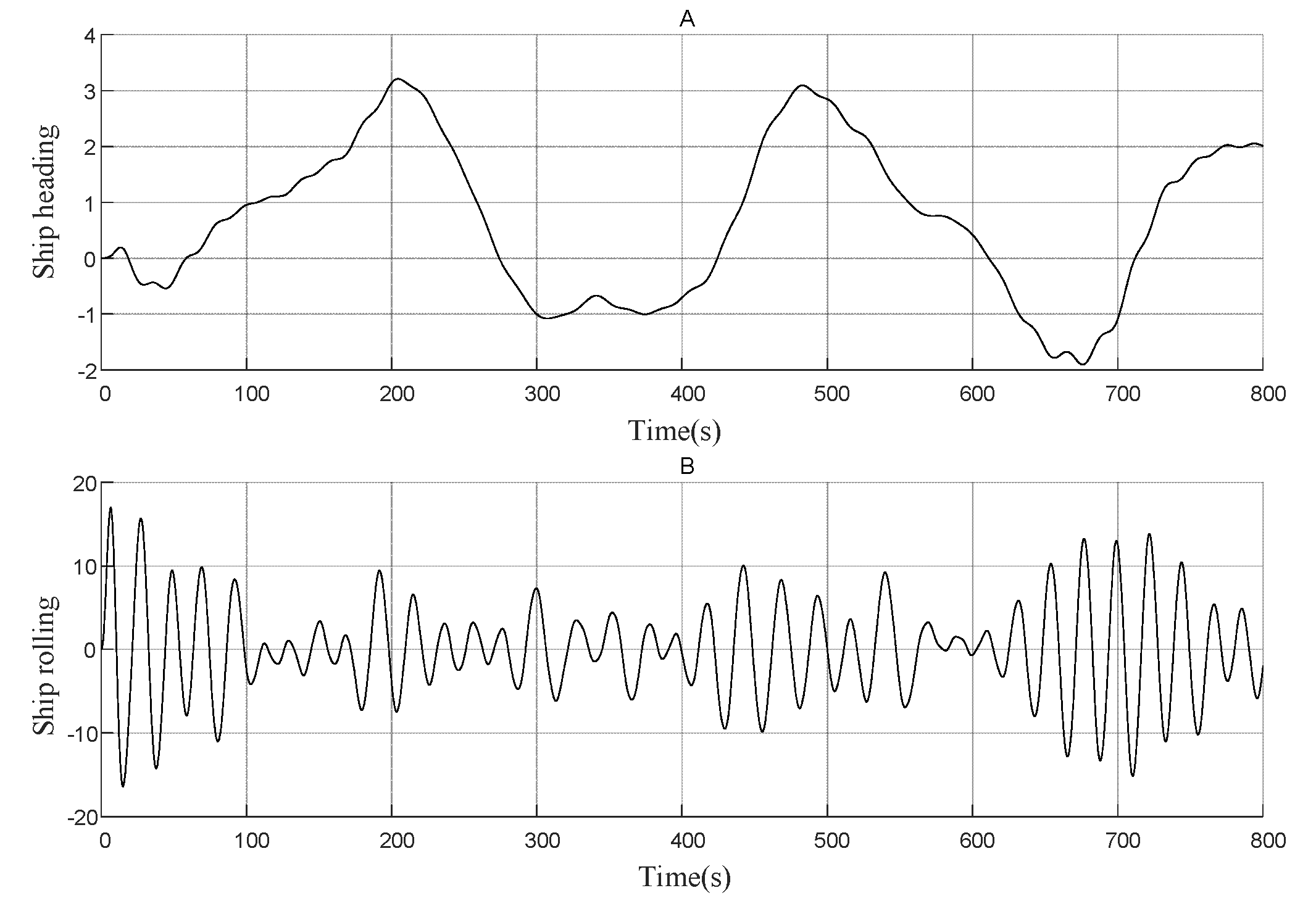
Figure 4.
Heading (A) and rolling (B) angles of the ship without control commands.

Figure 5.
Cooperative control effects of ship heading and rolling under signal attack. The simulation results of ship heading and rolling based on this control algorithm are shown by dotted lines in Figure A,B, respectively. Meanwhile the solid line in (A,B) depicts the heading and rolling output of the ship while the signal attack acted on the heading data signal. Here, the signal attack first happened at 80 s, and we have hi = 0.5. In addition, the operation states of main (flap) rudder and main (flap) fin are shown by solid (dotted) lines in (C,D), respectively.

Figure 6.
Data abnormalities of rudder and flap rudder. In (A,B), the abnormal data of ship rudder and flap rudder are first detected at 81.7 s and 80.4 s by Algorithm respectively.
Figure 6.
Data abnormalities of rudder and flap rudder. In (A,B), the abnormal data of ship rudder and flap rudder are first detected at 81.7 s and 80.4 s by Algorithm respectively.


Table 1.
Notations of Figure 2.
Table 1.
Notations of Figure 2.
| Annotation | Notations |
|---|---|
| Control objective | |
| Data from Sensor 3 | |
| Data sent by RTU 5 according to | |
| Data sent by DCU 3-1(2) according to | |
| Output of Actuator 1 sampling by Sensor 1 | |
| Data sent by RTU 1 according to | |
| Data sent by DCU 1-1(2) according to | |
| Output of Actuator 2 sampling by Sensor 2 | |
| Data sent by RTU 3 according to | |
| Data sent by DCU 2-1 according to | |
| Data sent by DCU 2-1(2) according to | |
| Control command for Actuator 1 by DCU 1-1(2) | |
| Data sent by RTU 2 according to | |
| Control command for Actuator 2 by DCU 2-1(2) | |
| Data sent by RTU 4 according to |
Table 2.
Influence of rolling mission by heading signal attack.
| Non-Attack | With-Attack | |||
|---|---|---|---|---|
| Mean | Variance | Mean | Variance | |
| Ship rolling | 7.95 | 10.01 | ||
| Fin angle | 45.71 | 54.37 | ||
| Flap fin angle | 164.05 | 184.35 | ||
Table 3.
Notations of rules.
| Annotation | Notations |
|---|---|
| DCU for ship rudders | |
| DCU for ship fins | |
| DCU for heading sensor | |
| DCU for rolling sensor | |
| Input register for rudder command | |
| Input register for flap rudder command | |
| Input register for fin command | |
| Input register for flap fin command | |
| Holding register for heading sensor | |
| Holding register for rolling sensor | |
| Set value of ship heading |
© 2018 by the authors. Licensee MDPI, Basel, Switzerland. This article is an open access article distributed under the terms and conditions of the Creative Commons Attribution (CC BY) license (http://creativecommons.org/licenses/by/4.0/).
Share and Cite
MDPI and ACS Style
Xing, B.; Jiang, Y.; Liu, Y.; Cao, S. Risk Data Analysis Based Anomaly Detection of Ship Information System. Energies 2018, 11, 3403. https://doi.org/10.3390/en11123403
AMA Style
Xing B, Jiang Y, Liu Y, Cao S. Risk Data Analysis Based Anomaly Detection of Ship Information System. Energies. 2018; 11(12):3403. https://doi.org/10.3390/en11123403
Chicago/Turabian StyleXing, Bowen, Yafeng Jiang, Yuqing Liu, and Shouqi Cao. 2018. "Risk Data Analysis Based Anomaly Detection of Ship Information System" Energies 11, no. 12: 3403. https://doi.org/10.3390/en11123403
Note that from the first issue of 2016, this journal uses article numbers instead of page numbers. See further details here.