Free Angular-Positioning Wireless Power Transfer Using a Spherical Joint


School of Electrical Engineering, Xi’an Jiaotong University, Xi’an 710049, China
*
Author to whom correspondence should be addressed.
Energies 2018, 11(12), 3488; https://doi.org/10.3390/en11123488
Submission received: 14 November 2018
/
Revised: 7 December 2018
/
Accepted: 11 December 2018
/
Published: 14 December 2018
(This article belongs to the Special Issue Wireless Power Transfer 2018)
Abstract
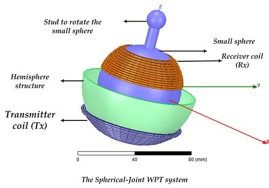
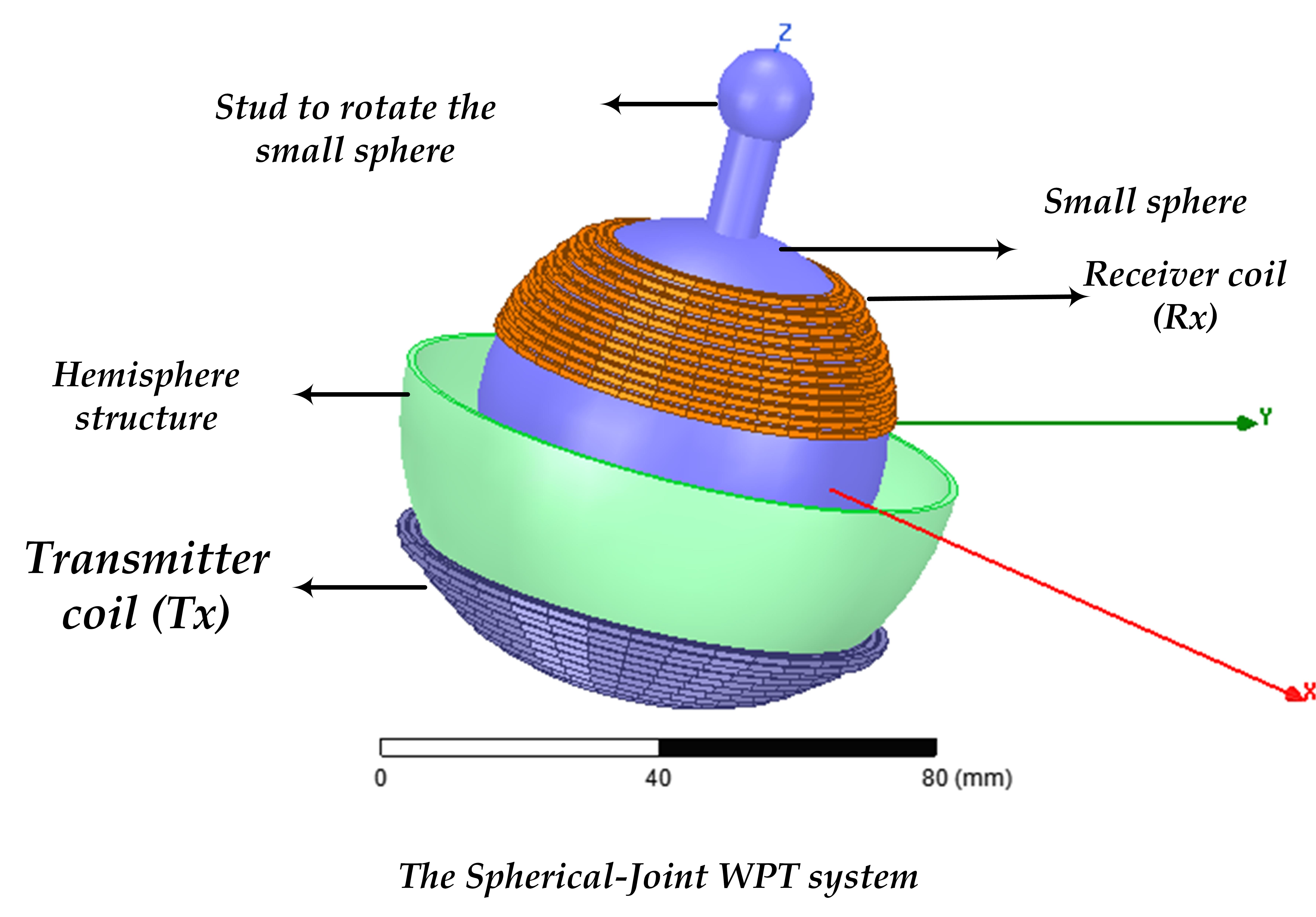
:Many studies have investigated resonator structures and winding methods. The aims of this paper are as follows. First, the paper proposes an optimized winding model for a bio-inspired joint for a wireless power transfer (WPT) system. The joint consists of a small spherical structure, which rotates inside a hemispherical structure. The transmitter coil (Tx) is wound on the hemisphere structure, and the receiver coil (Rx) is wound on the small sphere. The power is transferred while rotating Rx over a wide range of angular misalignment. In addition, the algorithm design of the proposed winding method is given to get an optimized model. Moreover, the circuit analysis of the WPT system is discussed. Second, the magnetic field density is investigated considering a safety issue, which is linked to human exposure to electromagnetic fields (EMFs). Moreover, EMF mitigation methods are proposed and discussed in detail. Finally, the simulation results are validated by experiments, which have confirmed that the proposed winding method allows the system to rotate up to 85 degrees and achieve an efficiency above 86%. The proposed winding method for the WPT system can be a good technique for some robotic applications or a future replacement of the human joint.
1. Introduction
Wireless power transfer (WPT) systems have become a widely used technology. They are used to transfer the power for many applications in many fields, such as electric vehicle (EV) charging [1,2,3], plug-in hybrid electric vehicles (PHEVs) [4], implantable medical devices (IMDs) [5], consumer electronics [6], autonomous underwater vehicles (AUVs) [7], and robotic systems [8]. Wireless power technology is also used in communication networks [9,10,11]. In addition, Internet of Things (IoT) is the key part of evolving the wireless communication environment. IoT presents a developing topic of great technical and economic significance [12,13].
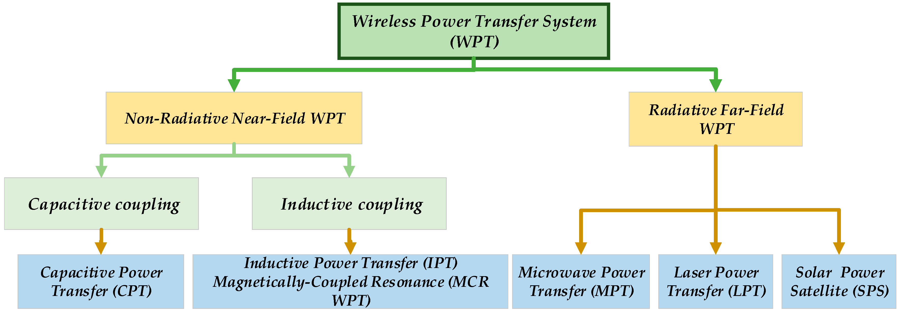
WPT technology can be divided into two categories. The first is radiated far-field WPT, which includes microwave power transfer (MPT) [14], laser power transfer (LPT) [15], and a solar power satellite (SPS) [16]. The second is non-radiated near-field WPT, which comprises inductive power transfer (IPT) and capacitive power transfer (CPT). Figure 1 illustrates the classifications of the WPT system.
Many studies have investigated coil structures that are used in a wide range of applications, such as flat coils, square coils, and coils with cores. Three-dimensional structures have also been discussed, for example, a bowl-shaped transmitter coil [17]. The three-dimensional resonant cavity has been discussed, offering an effective way of charging multiple devices simultaneously, such as devices implanted in a freely moving animal [18], charging a mobile phone and a watch [19], and LEDs [20]. Helical-type coils made of superconductors are presented to increase the quality factor of coils [21]. Moreover, omnidirectional WPT systems are given in [22,23], and the 3D structure for a three-phase WPT system is discussed in [24]. The three-phase WPT system has found its way to some practical applications [25]. In [7], a three-phase charging system is proposed and used to recharge an autonomous underwater vehicle (AUV). In EV power charging, the resonators are designed as circular, planar, or square coils [26]. Moreover, dipole-type coils with cores [27], defected ground structures (DGS) [28], cross-shape structures [29], and L-shaped coils [1,30] are given. Many other structures are reported in [31].
Figure 2 shows several WPT coils’ structures. Most of the WPT systems consider fixed Tx and Rx structures. However, in real applications, there might be a misalignment, which differs randomly under different situations or different application types. For example, during EV charging, if there is imperfect parking, there will be a misalignment between Tx and Rx. As a result, several parameters could change, such as mutual inductance, efficiency, and output power. Therefore, Rx is intentionally moved to obtain horizontal, vertical or angular misalignments in order to study the effect of these movements on the performance of the WPT system [32]. In [33], the angular, general, and lateral misalignments are applied to a helical coil and, as a result, the mutual inductance varies with the misalignment, which further results in fluctuations in output power and power transmission efficiency (PTE). In [34], with misalignment of the coils, mutual inductance rapidly changes. On the other hand, some studies have investigated structures with moving coils. For example, in [35], the authors proposed a ball-joint structure, where the ball can rotate inside a socket structure while transferring the power. Moreover, linear-motion transmission for a robot is proposed [8], and this structure is appropriate for the applications that involve a linear movement.
Joints are basic parts of robots, such as humanoid and industrial robots. Moreover, the human body has many joints. Therefore, artificial joints have been used as a replacement for damaged ones, such as in total knee replacement (TKR) with sensor-equipped support, which has become an increasingly common surgery worldwide [36,37]. The joint has a specific mission to cause either a movement or a rotation. In this paper, we use a bio-inspired joint structure for the WPT system similar to the hip joint and the glenohumeral joint of the shoulder.
In this paper, we propose a winding method for Tx and Rx. The proposed winding method permits a small sphere to rotate inside a hemispherical structure over a wide range of angular rotation while maintaining a high PTE. The algorithm was designed to achieve the optimal model of the proposed winding method. Modeling and simulations of five winding methods were conducted and compared based on the fluctuation of the mutual inductance and coupling coefficient when Rx rotates inside Tx. Magnetic field density is investigated in detail considering the safety issue, which is linked to the human exposure to EMFs. To ensure the safety and reliability of the proposed system, two EMF-mitigation methods are proposed, and the advantages and disadvantages of these methods are given. The study proves that a thin metallic shield of aluminum up to 0.3 mm can suppress the EMFs around the coils. The generated magnetic field density was about 5.14 µT, which complies with the International Commission on Non-Ionizing Radiation Protection (ICNIRP) 2010 guidelines. Finally, several experiments are put forward to validate the simulation results and analyze the WPT performance. The measurements validated the simulation results and proved that the optimized model reduced the fluctuation of the mutual inductance. The mutual inductance was between 3.5 µH at α = 0° and 4.5 µH at α = 85°. As a result, the efficiency could be maintained at up to 86% at α = 85°. The proposed winding method for the WPT system is a good choice to transfer the power efficiently across the gap.
This paper is organized as follows. In Section 2, an optimized design of the proposed windings is presented. Moreover, the circuit analysis of the joint WPT is analyzed. In Section 3, modeling and simulation of several WPT windings are presented and compared. In Section 4, the magnetic field density for several models considering human exposure to EMFs is discussed. In addition, EMF mitigation methods are given and compared. Finally, Section 5 presents the experimental setup of the WPT system. The measurements are implemented to validate the obtained results, and a discussion is provided.
2. Optimized Design Method of the Joint WPT System
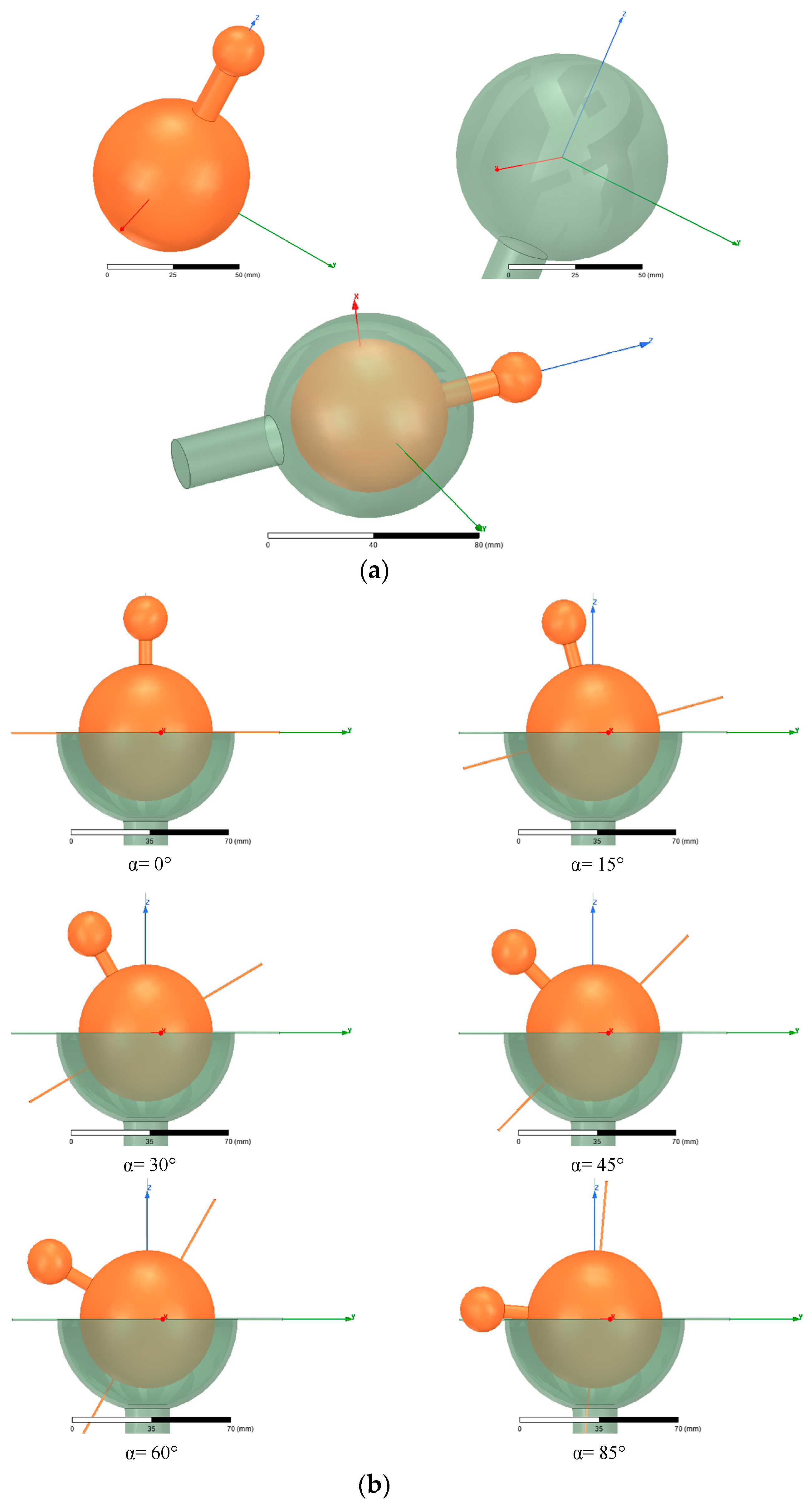
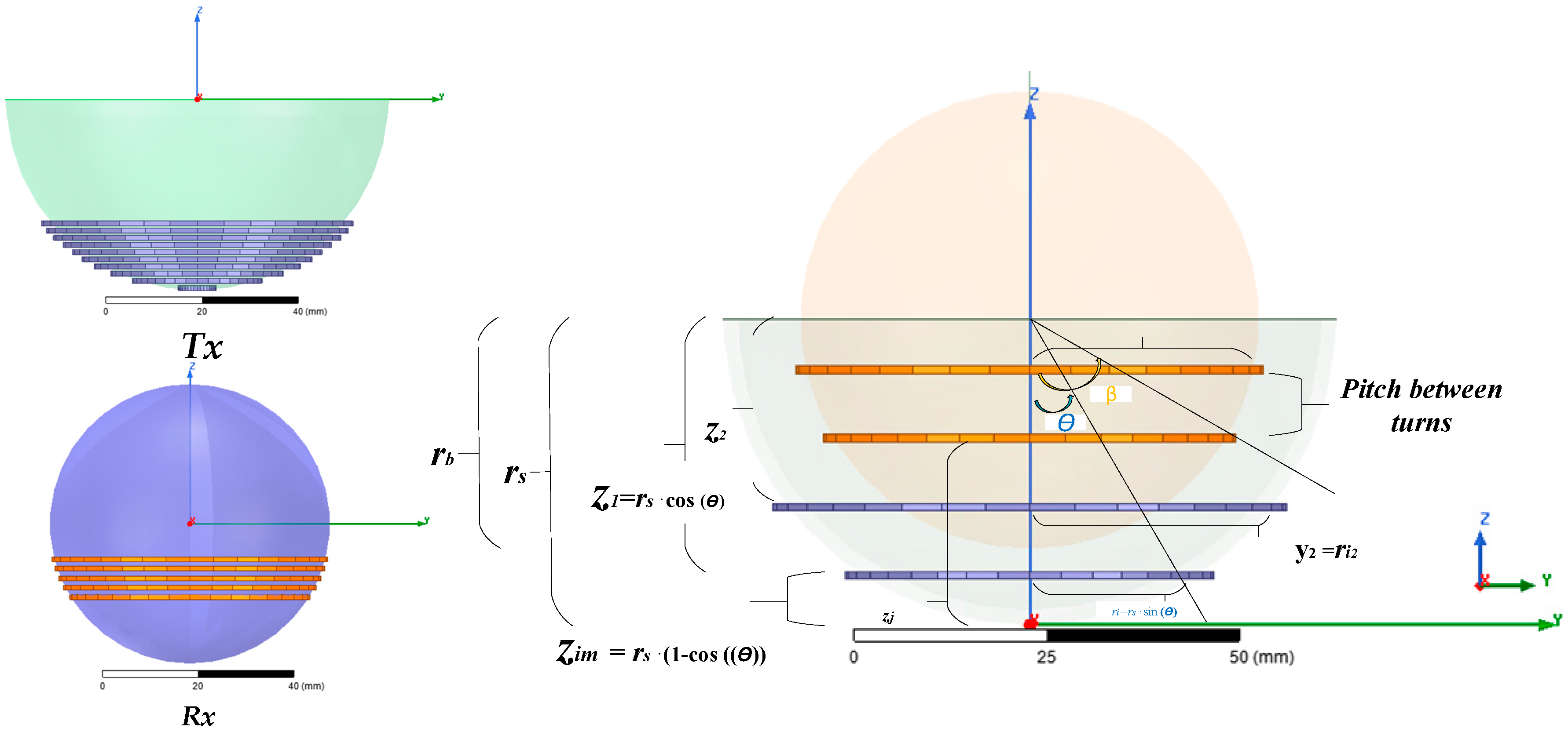
The spherical joint consists of two sphere-shaped structures. Tx is wired on a large spherical structure as shown in Figure 3a, or wired on a hemispherical structure as illustrated in Figure 3b. Rx is wired on the small sphere, and can rotate inside the large sphere using a mechanical stud. The angle α represents the angle between the vertical axes of both structures. The spherical structure for Tx requires a slot for the stud to go through and thus allow the rotation of the small sphere. However, the degree of rotation is limited between 0° and 45°. On the other hand, in case of a hemispherical structure for Tx, the angular displacement of the small sphere is between 0° and 85°.
Figure 3c illustrates the dimensions of the joint structure. The receiver radius is 2.85 cm, which can be appropriate for some robotic applications that vary in size. However, considering the use of this structure as a potential replacement of the human body joint, the size needs to be reduced. In this case, a high frequency can be used, such as the industrial, scientific and medical (ISM) band for IMDs (2.2 MHz).
2.1. Design Method and Algorithm Design
PTE is considered a key design factor of the WPT system while operating at the resonance frequency. The PTE optimization between coils depends on the coupling coefficient, which is given by where M is the mutual inductance. M is proportional to the square root of the transmitter and receiver inductances L1 and L2, respectively. The inductance is related to the coil geometry, which includes the size of the resonator, the radius of Litz wire and its cross-sectional area, the length, the number of turns and layers, and the separation between turns. Therefore, the PTE is optimized by changing the shape of winding coils in order to maximize the mutual inductance and reduce its fluctuation during the angular displacement. Of note, the coupling coefficient should stay within a certain range to avoid cases with very low values or cases with very high coupling between Tx and Rx. Several variables are considered to parametrize the coils, such as the number of turns, layers, space between turns, and variation in the z-axis position.
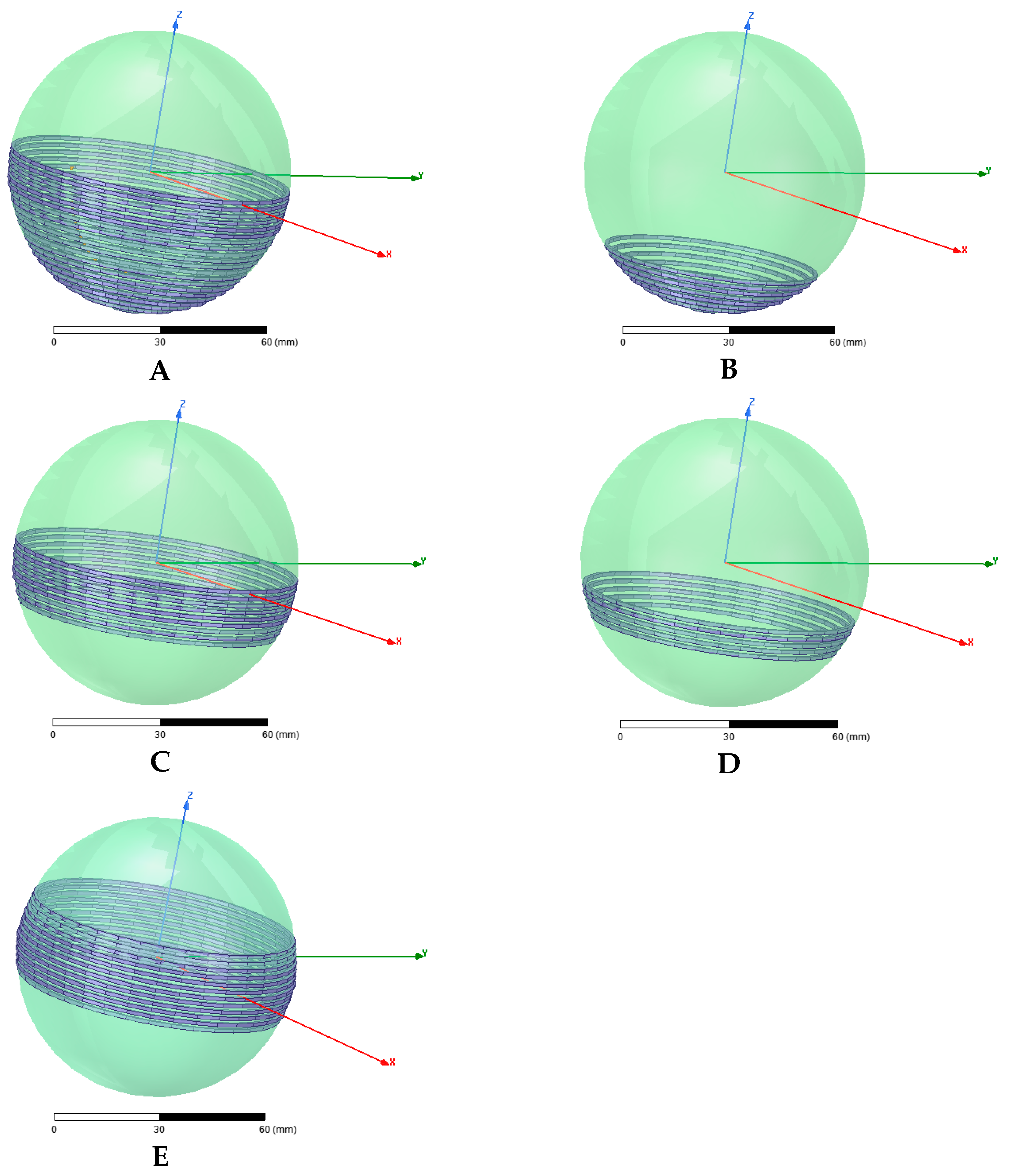
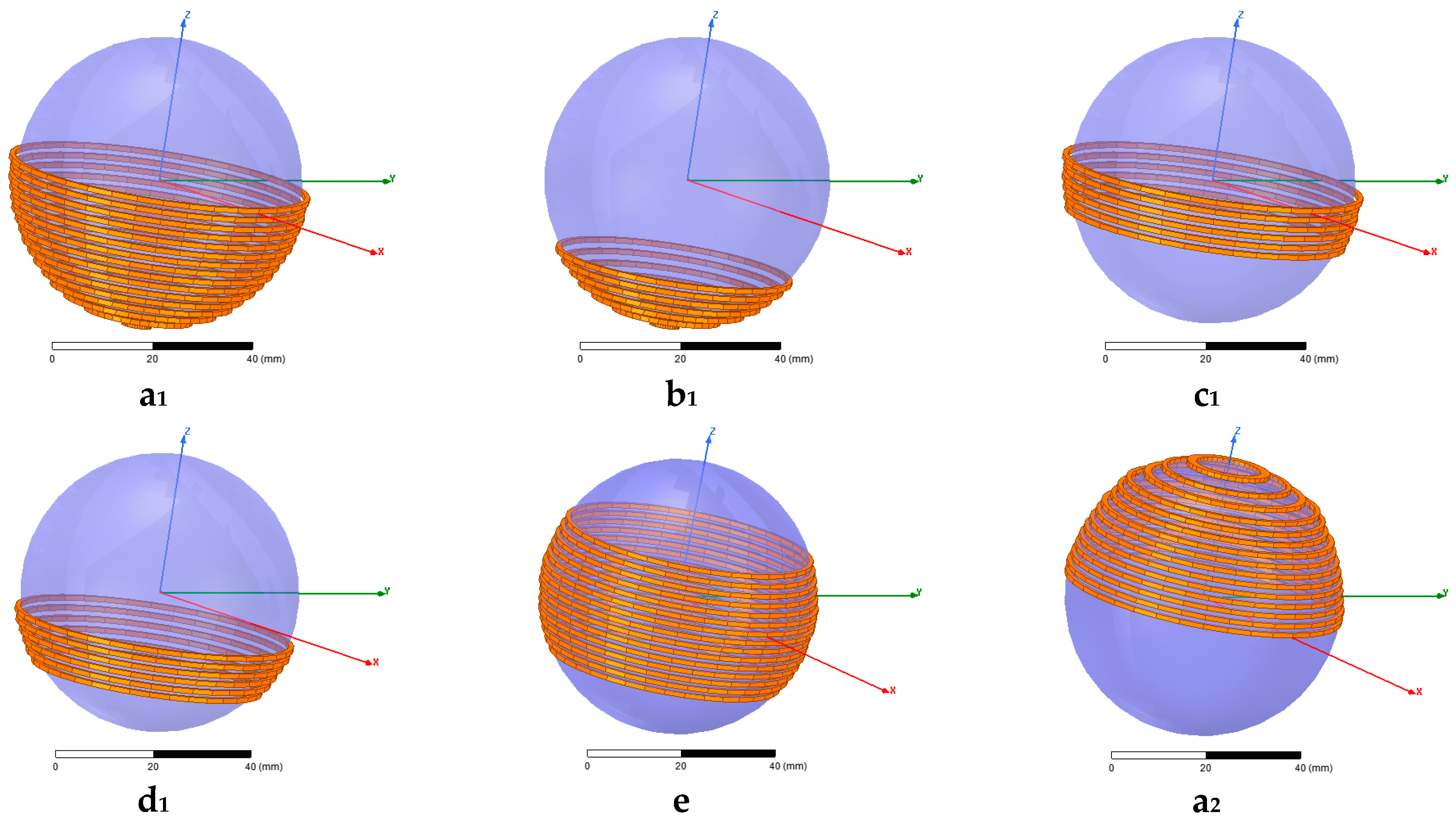
There are many possibilities to wind the coils on the joint structures. Figure 4 illustrates five basic cases of Tx windings (A–E). Cases (A–D) are wound on the hemispherical structure. Case (E) is a special case where Tx is wired on the spherical structure. Figure 5 shows nine cases of Rx windings (a1–e) and (a2–d2). If the abovementioned cases are combined together, 45 cases with different winding methods will be obtained. Table 1 displays the combination methods of Tx and Rx, and they are as follows. The cases shaded in blue have low coupling coefficients (loosely coupled), such as Bb2 and Bd2. The cases shaded in green have high coupling coefficients (tightly coupled), such as Aa1, Cc1, Ee, and so on. Finally, the cases shaded in white have average coupling coefficients.
The joint–WPT system in Figure 6 is assumed to be on the y-z plane. The transmitter coil has N1 turns, and the receiver coil has N2 turns. ri is the radius of each horizontal turn of the transmitter coil at zi (z-position). rj is the radius of each horizontal turn of the receiver coil at zj (z-position). The radius of the transmitter and receiver coils are already given by rs = 3.85 cm and rb = 2.85 cm, respectively.
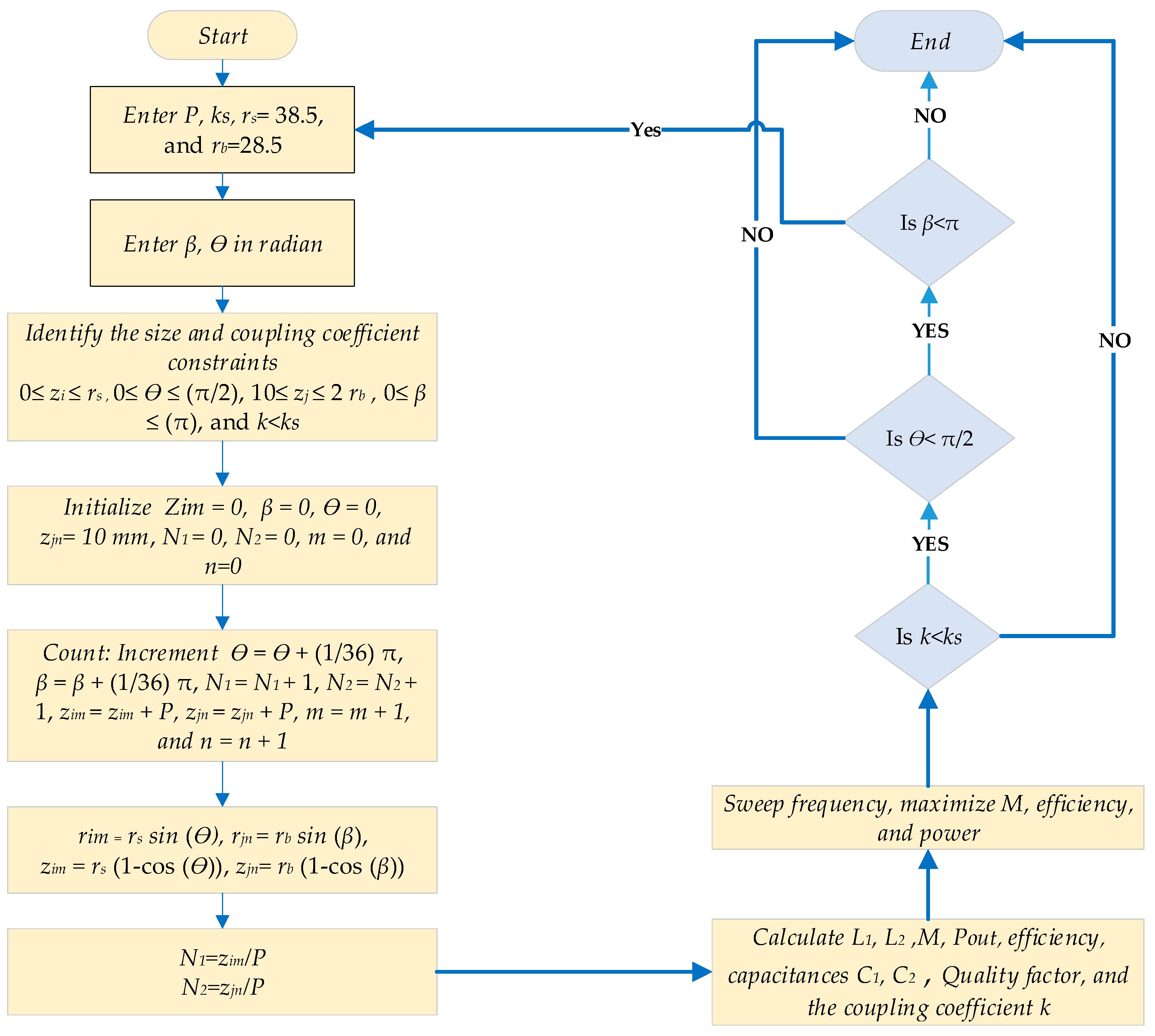
The algorithm design was written and can be represented by a flowchart, as illustrated in Figure 7. The flowchart shows the algorithm steps and their order to get an optimized model taking into account some constraints. The steps are as follows:
- Enter the radius of the transmitter coil rs = 38.5 mm, the radius of the receiver coil rb = 28.5 mm, and pitch between turns P = 0.5 mm.
- Enter β,. // (radian).
- Size constraints: 0 ≤ zim ≤ rs; the turns can cover the whole space of the hemisphere of the transmitter structure, which means: 0 ≤ ≤ (π/2). On the other hand, 10 ≤ zjn ≤ 2 rb; the turns can occupy the whole space of the sphere, which means: 0 ≤ β ≤ (π). Moreover, zim and zjn are the z-position of the transmitter and receiver turns, respectively.
- Initialize zim, β, and as 0. Initialize zjn = 10 mm (start the z-position for Rx), N1 = 0, N2 = 0, m = 0, and n = 0.
- Count: = + (1/36) π, β = β + (1/36) π, N1 = N1 + 1, N2 = N2 + 1, zim = zim + P, and zjn = zjn + P. In addition, m = m + 1, n = n + 1. // Increment angles to determine the z-position and radius for each turn of the transmitter and receiver windings ((1/36) π is the assumed step). Increment N1, N2 to find the number of turns for both coils. Move the turns in the z-direction with the pitch between coils equal to 0.5 mm. The number of turns can be calculated by N1 = zim/P and N2 = zjm/P.
- Calculate rim = rs sin (), rjn = rb sin (β), zim = rs (1 − cos ()), zjn = rb (1 − cos (β)). //mm (based on angles). rim and rjn are the radii of the transmitter and receiver turns, respectively.
- Calculate L1, L2: the self-inductances of the transmitter coil and receiver coil, respectively. Calculate and maximize the mutual inductance M, calculate the coefficient coupling k, and determine the required capacitors C1, C2. // In order to maximize the mutual inductance, the inductances will be adjusted based on the number of turns and the space between turns (pitch). The transferring distance between Tx and Rx will determine the coupling coefficient, which should be less than a certain value ks.
- With the available value of the frequency and calculated resistances (R1 for Tx and R2 for Rx), calculate the quality factor, transferred power, and efficiency.
- Sweep the frequency and mutual inductance to maximize the efficiency and transferred power.
- Is k < ks, if yes go to 11, or else go to step 13. // The coupling coefficient should stay within a certain range to avoid cases with very low values or cases with very high coupling between Tx and Rx.
- If < π/2 go to step 12, else go to step 13.
- If β < π, go to step 2, else proceed to step 13.
- End.
2.2. Circuit Analysis
Figure 8a shows the magnetically coupled resonance (MCR) WPT system, and Figure 8b presents the equivalent circuit in series–series (SS) mode. The transmitter and receiver resonators are represented by inductances L1 and L2, respectively. R1 is the resistance of Tx and R2 is the resistance of Rx. In addition, C1 and C2 are the resonance capacitors.
The Neumann expression for the mutual inductance between two coils is given as [35]:
Lm,n is the inductance between coils m and n. H/m is the magnetic permeability of vacuum, and Xm, Xn are the infinitesimal length vectors along m and n, respectively. In case of m = n, the self-inductance is calculated. If we consider a circular coil consists of many loops, for the ith loop with a radius ri and cross-sectional area of ai, the self-inductance can be given as follows [17]:
Additionally, the mutual inductance between coaxially arranged circular loops is given by:
where ri and zi are the radius and position on the z-axis for the ith coil, respectively. rj and zj are the radius and position on the z-axis for the kth coil, respectively. is the complete elliptic integral of the first kind, and is the complete elliptic integral of the second kind.
In this paper, the coils are coaxially arranged. Therefore, the total inductance of the transmitter coil LTx is the summation of the self-inductances of the transmitter loops and the mutual inductance between these loops in addition to the mutual inductance between the transmitter and receiver coils as shown below:
where is the mutual inductance between the transmitter and receiver coils. In a similar way, the receiver inductance is obtained by:
The output power and output voltage of SS-compensated WPT can be given as follows:
The output voltage is linearly dependent on the load resistance RL. The efficiency is given by Equation (11), and the SS-compensated WPT can be designed at the maximum mutual inductance.
3. Simulation Results
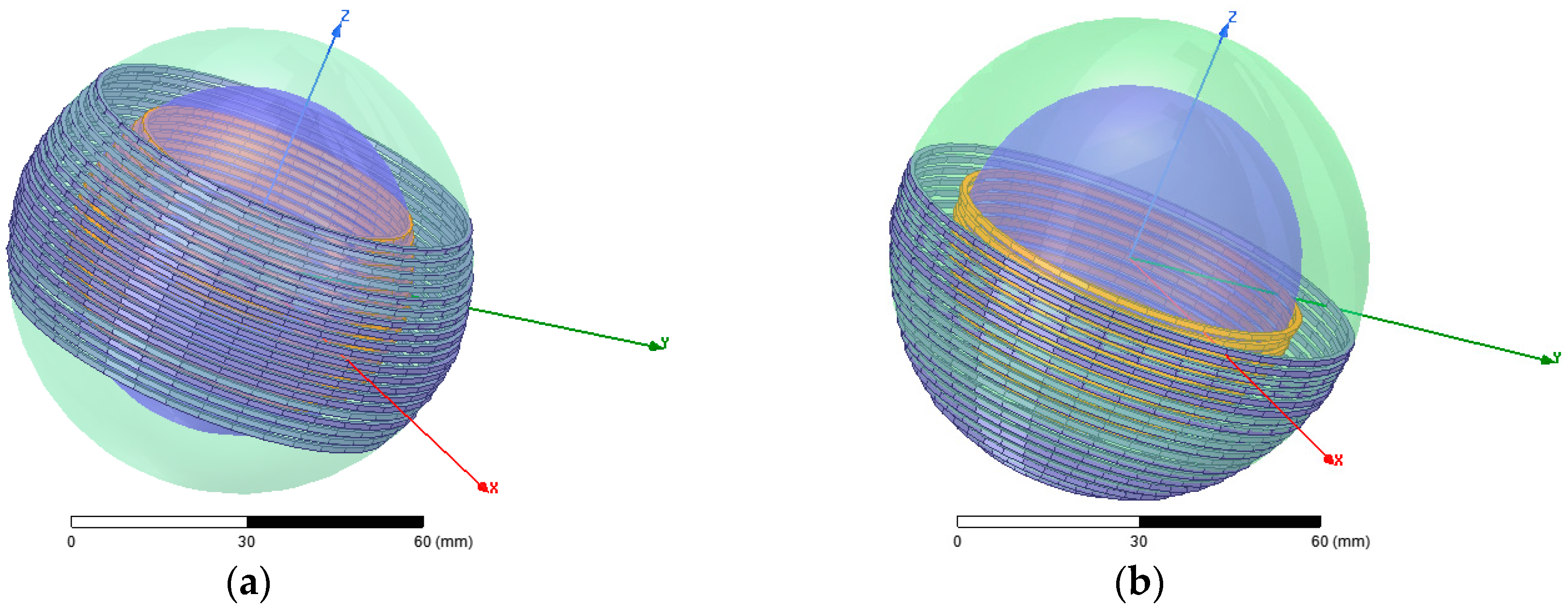
Based on the required value of the coupling coefficient ks, the optimization process can result in many possibilities, and some cases are chosen for comparison purposes. Figure 9a,b shows the equator windings and hemisphere windings, respectively. At zero-degree angle, the equator and hemisphere cases have very high coupling coefficient above 0.50. Double-layer windings, which is presented in Figure 9c, has a coupling coefficient of 0.2. Figure 9d illustrates a modified hemisphere winding. Finally, the optimal model is shown in Figure 9e with k = 0.089. In our study, in order to ensure accurate work, the simulations of the joint WPT system are conducted by ANSYS Electronics 19.0.0 (Canonsburg, PA, USA; Ansys Maxwell 3D to simulate the joint–WPT system and Ansys Simplorer for co-simulation). The obtained parameters are given in Table 2.
Figure 10 displays the fluctuations of the mutual inductance and coupling coefficient due to the rotation of Rx (angular misalignment α). In the case of equator windings (Figure 10a) and hemisphere windings (Figure 10b), the mutual inductance will drop when the angular misalignment increases, which, in turn, leads to a very low efficiency, particularly at high rotation degrees close to 85°. In the case of double-layer windings for Tx and Rx (Figure 10c), the performance of the WPT system will improve. However, the fluctuation of the mutual inductance is still high. For the optimal model (Figure 10d), the fluctuations of M and k are reduced. Therefore, the performance of WPT is greatly improved. As a result, the receiver can rotate inside the transmitter from zero degrees, which means perfectly aligned coils (α = 0°), up to 85° while maintaining high efficiency.
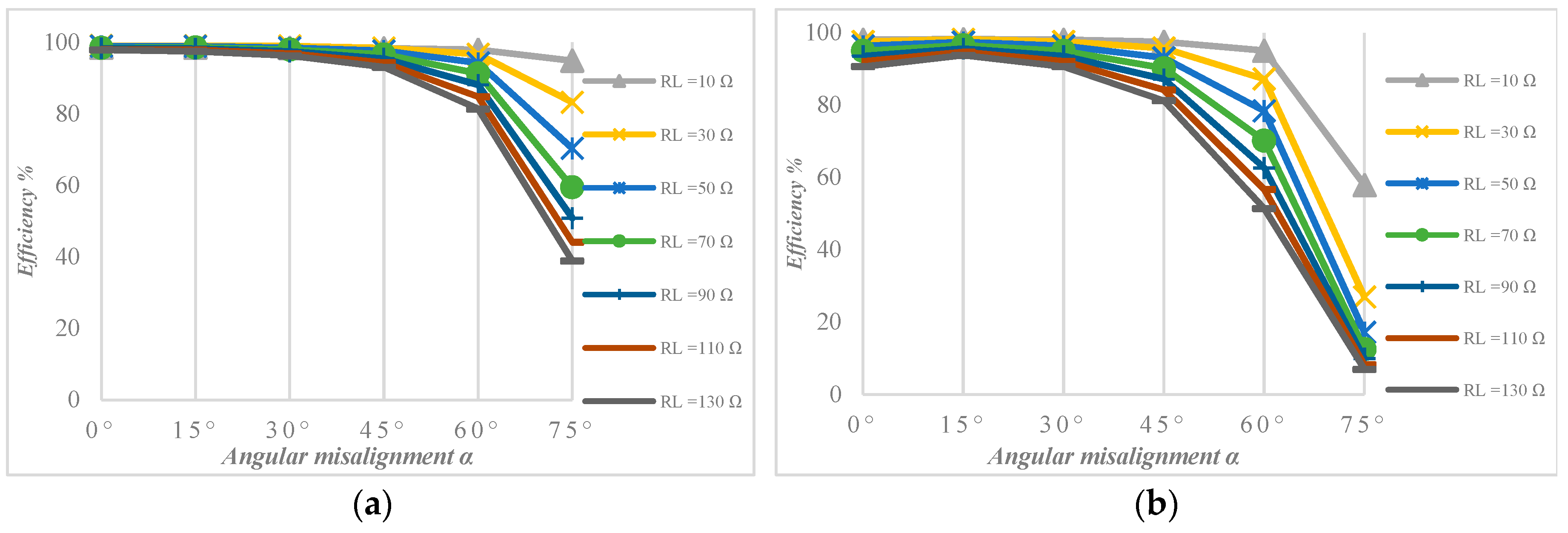
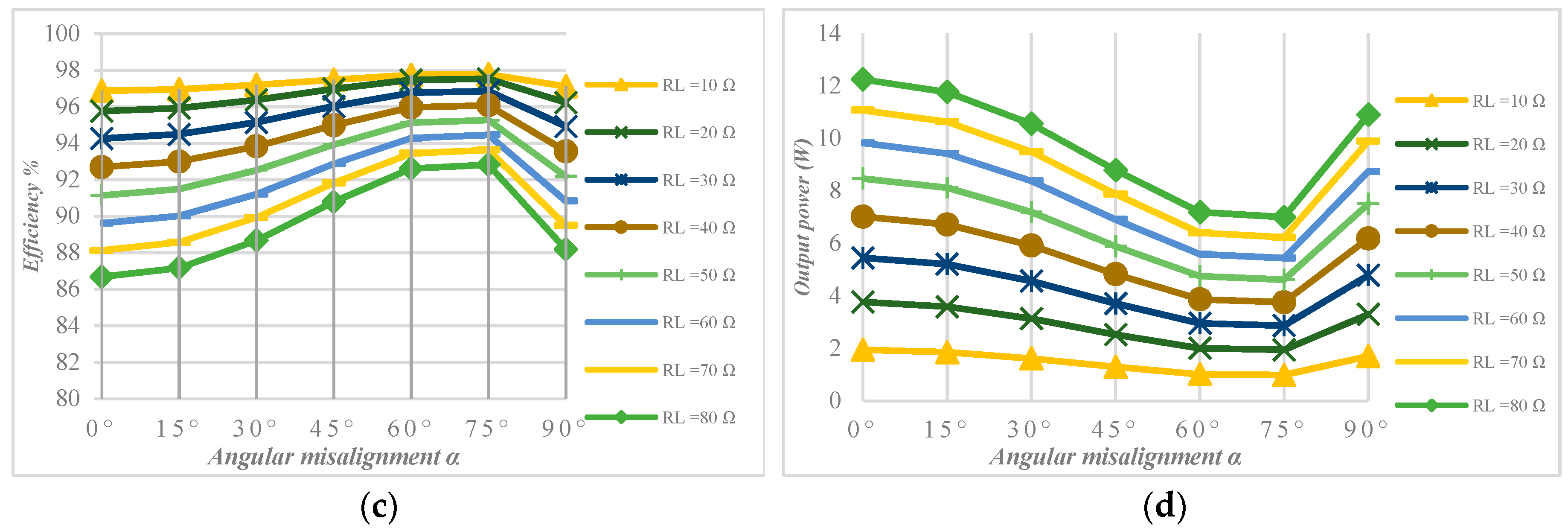
To provide a clear picture, the relationship between the efficiency, load, and angular misalignment is clarified in Figure 11. In the case of equator windings (Figure 11a) and hemispherical windings (Figure 11b), efficiency drops fast after 45°. For example, in the case of equator windings at α = 75° and a load of RL = 50 Ω, the efficiency is about 62%. However, at α = 85°, the efficiency will be less than 10%. For the hemisphere windings at α = 75° and RL = 50 Ω, the efficiency is 18%, while at α = 85°, the efficiency will be very close to zero. On the other hand, in the case of optimal design of the WPT system (Figure 11c), the efficiency is up to 95% at α = 75°, and almost 93% at α = 85°. The output power of the optimal model is presented in Figure 11d. As given in Equation (9), the output power is proportional to the load value and input voltage. However, it is inversely proportional to the square of the mutual inductance.
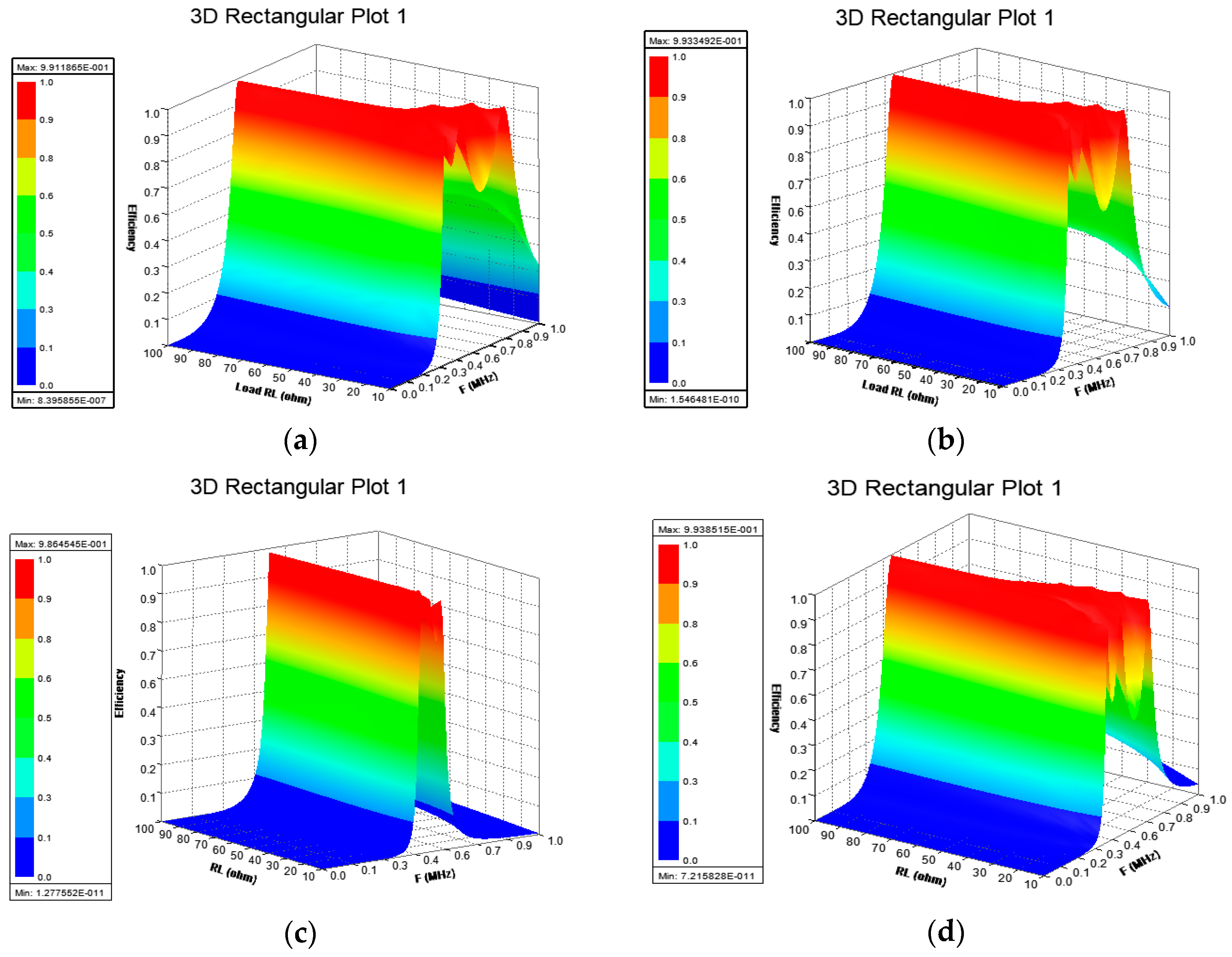
Finally, Figure 12 presents the relationship between the efficiency, load, and resonant frequency for the five case studies (Table 2). Different winding methods resulted in different transferring distances, and thus different coupling coefficient values were achieved. When Tx and Rx are close enough to each other, the coupling becomes stronger, and as a result, a frequency-splitting problem might occur. Therefore, the resonant frequency will change and the output power will drop. The hemisphere and modified hemisphere windings are similar to each other as shown in Figure 12b,d. In the case of double-layer windings (Figure 12c), the system shows more stability for load values above 50 Ω. On the other hand, the optimal model (Figure 12e) is steady enough even at low load values, and this will ensure high power transfer and efficiency.
4. Magnetic Field Density of the WPT System and Mitigation Methods
The WPT system (according to the application type) can be positioned close to the human body or other sensitive circuits. Therefore, the design of the WPT system should be in accordance with the WPT-related standards. Several standards have been issued by international organizations, for example, the International Commission on Non-Ionizing Radiation Protection (ICNIRP 2010); IEEE Standards; Federal Communications Commission (FCC) in the USA; China Communication Standard Association (CCSA); and Broadband Wireless Forum (BWF) in Japan [31,38].
4.1. Magnetic Field Density
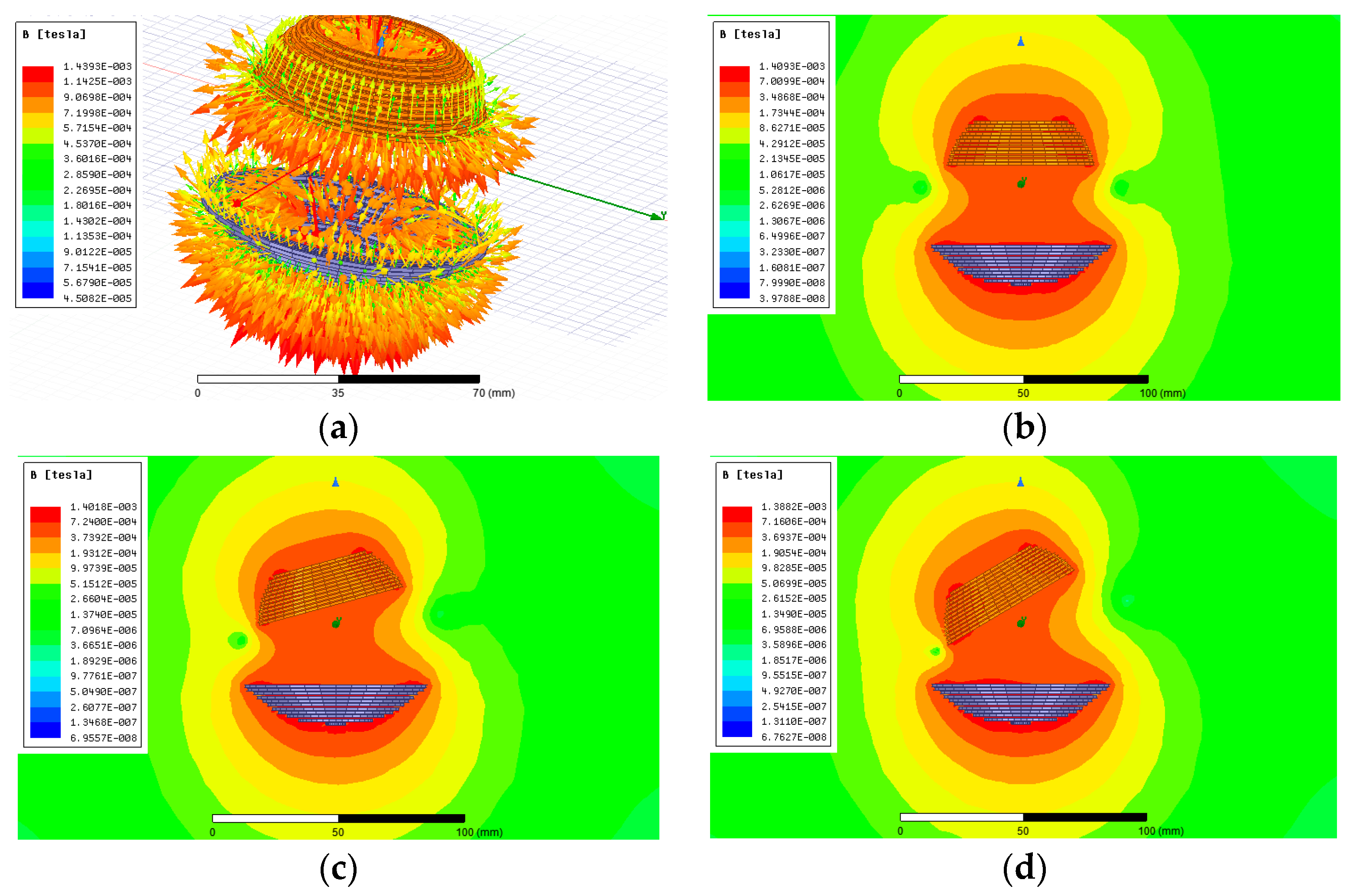
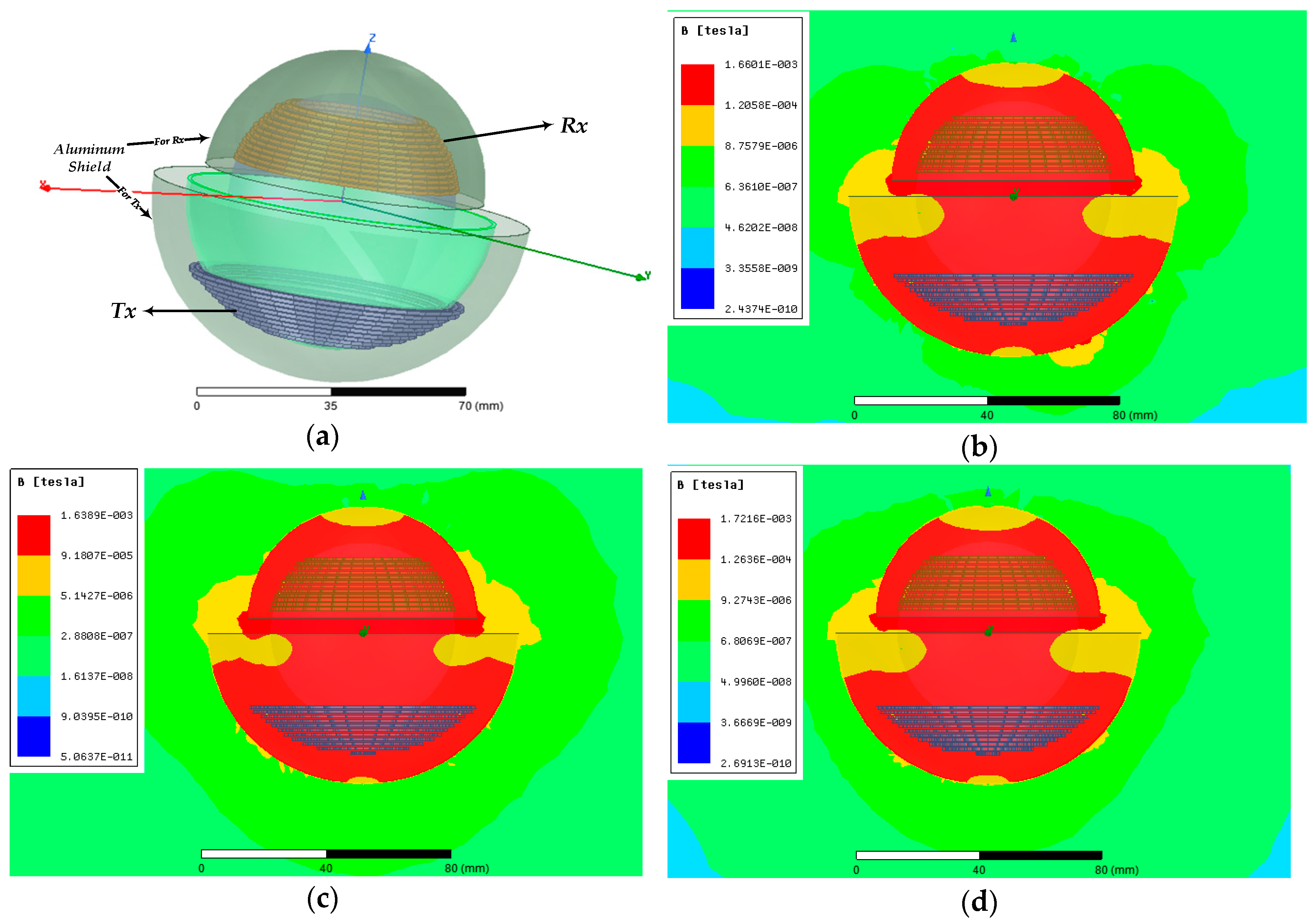
In 2010, ICNIRP introduced guidelines in order to limit the exposure levels to EMFs, which should not exceed 27 μT. The magnetic field density (B) of the optimal model is presented in Figure 13. The magnetization direction is displayed in Figure 13a. The magnetic field density is given by B = µH, where H is the magnetic field strength (intensity) and measured by (A/m). In Figure 13b, at α = 0°, the yellow area (within 12 cm diameter) shows that B is around 86 µT, which is greater than the allowed level according to ICNIRP 2010. On the other hand, the green area is almost safe with an average B value up to 15 µT.
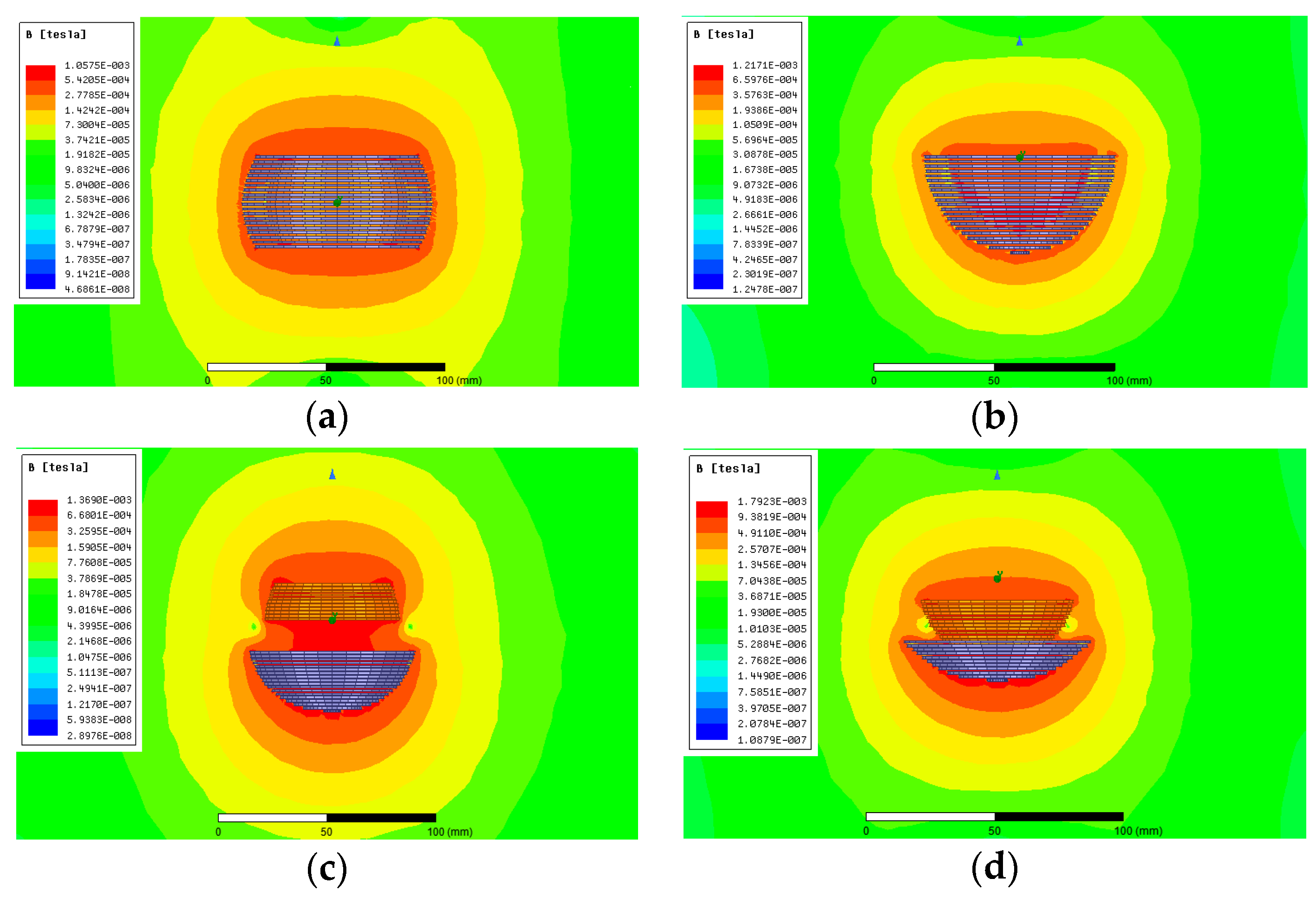
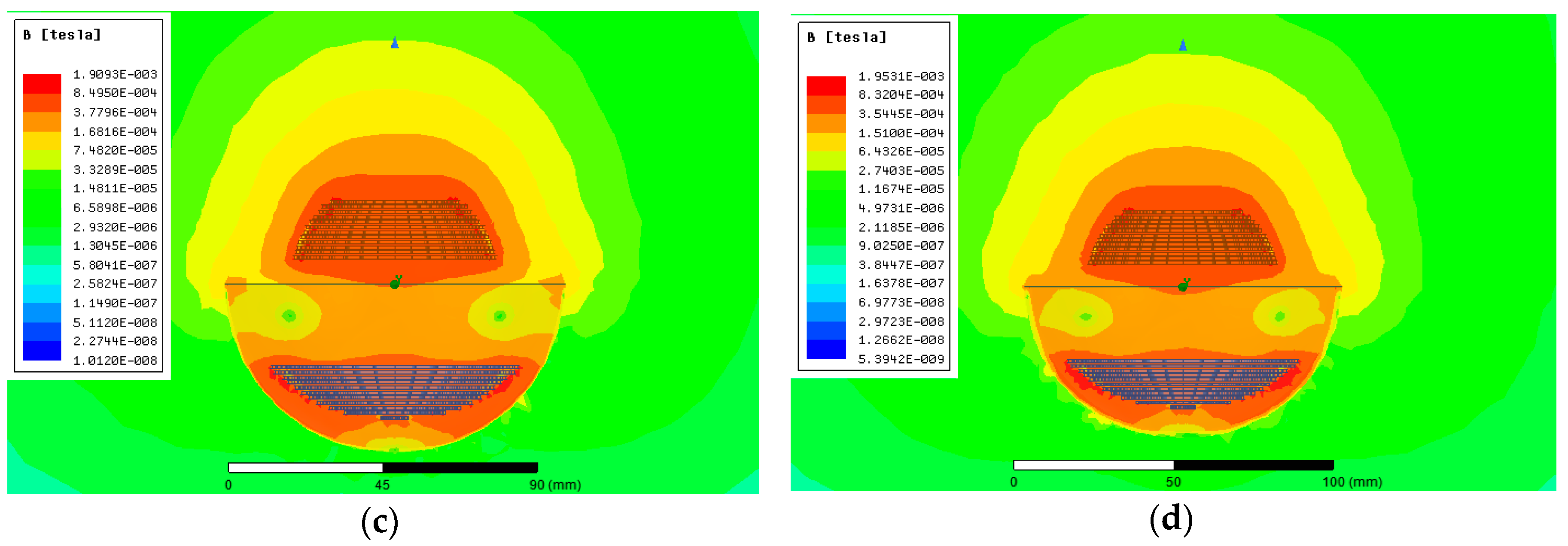
Based on the magnetic field density, a comparison between the five cases (see Figure 9) is illustrated in Figure 14. It is obvious that the dark green zone around the joint WPT in all the models is within the standard limit. However, the yellow area around the joint displays values above the limits. The hemisphere windings (Figure 14b) and modified hemisphere windings (Figure 14d) have the highest values, and reach 105 µT and 121 µT, respectively. Nevertheless, attention should be concentrated on the optimal model, which is the basic case.
4.2. Mitigation Methods
The EMF mitigation method is chosen based on the cost, weight, and size constraints of the application; for example, choosing ferrites is not a good choice since it will put more pressure on the robotic arm. In this paper, two methods are discussed and compared. The first is active shielding, and the second uses metallic shielding.
4.2.1. Active Shielding
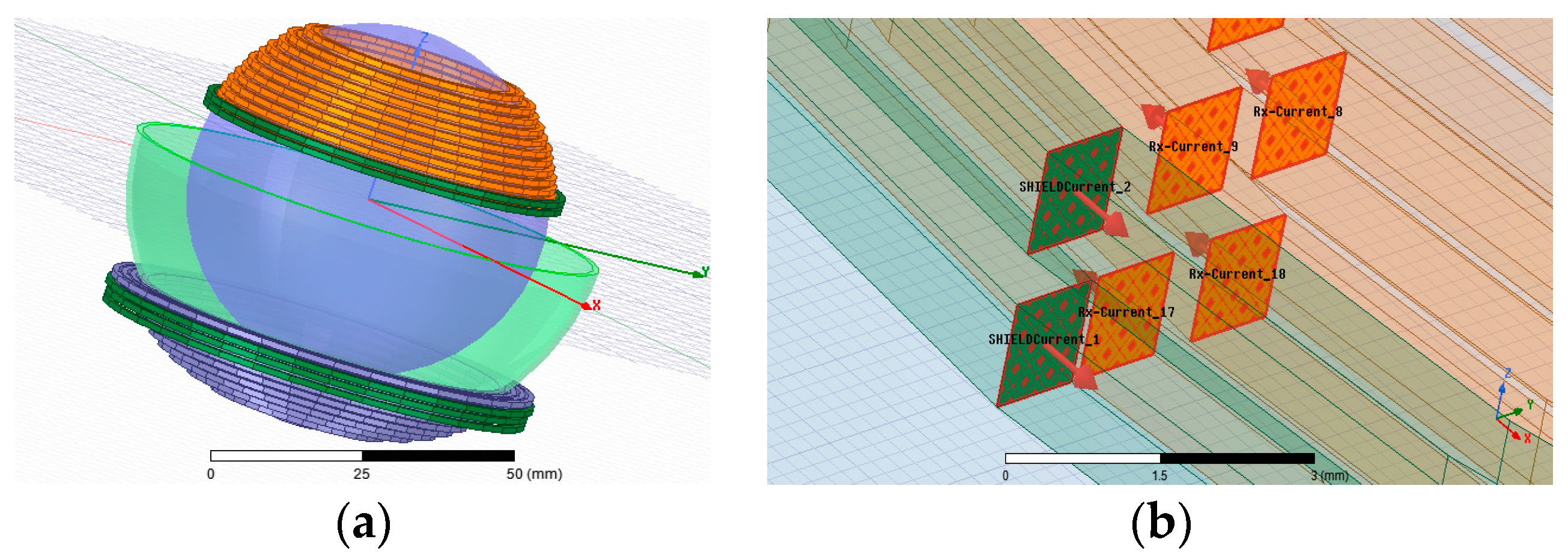
The shielding coils are part of the WPT coils and the same current flows in both coils. As illustrated in Figure 15a, two turns were taken. The shielding coils are wound in opposite direction to Tx and Rx. Therefore, the currents that flow in the shielding turns are opposite to the currents that flow in Tx and Rx as presented in Figure 15b. Therefore, the generated magnetic field (MF) by shielding coils opposes the generated MF by WPT coils.
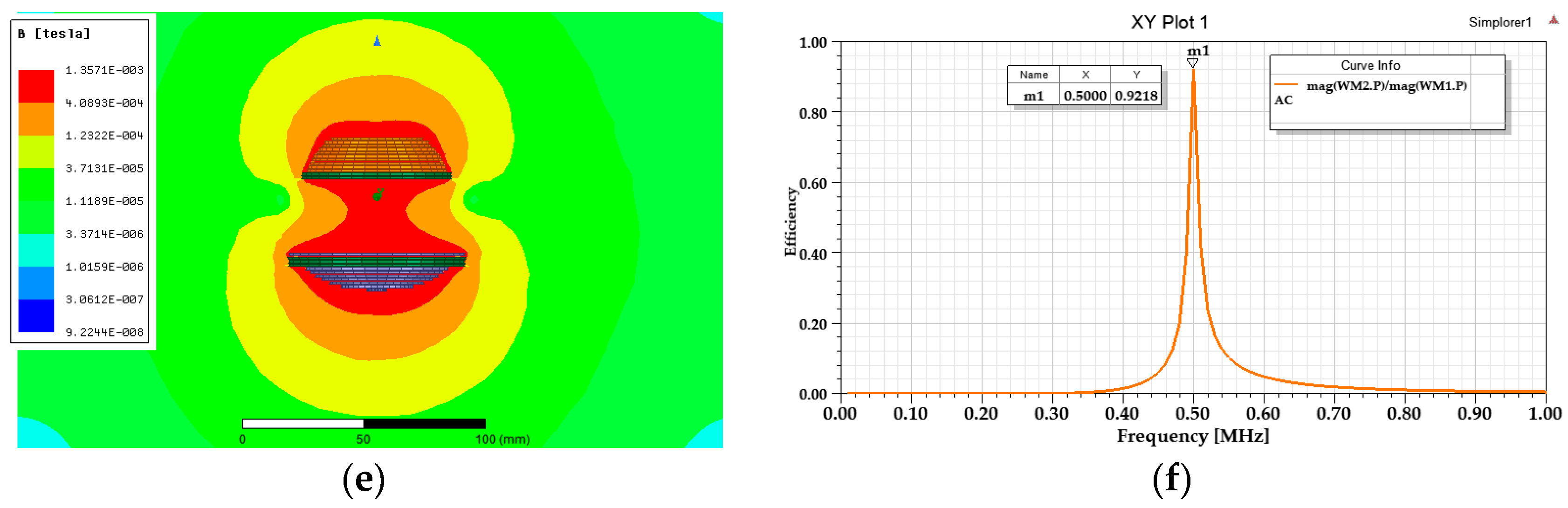
Figure 16a,b displays the magnetic field density and efficiency at a load of 50 Ω for the WPT system without shielding coils. As shown in Figure 16c, the leakage MF is reduced from 102.73 µT (without shielding) to 96.75 µT. However, the inductances of Tx and Rx in addition to the mutual inductance are decreased. Thus, the obtained PTE dropped from 95.26% (without shielding) to 91.15% with the shielding coils (Figure 16d). Moreover, the current in this method is dependent on the WPT current, which is variable. In the second case, the cancelling coils are separated from the WPT coils, which means they do not have the same current. Therefore, the inductances of WPT coils and the mutual inductance do not change. However, the MF around the joint has changed as shown in Figure 16e. In addition, a drop of efficiency has occurred (from 95.26% to 92.18%) as presented in Figure 16f. By increasing the number of turns of the shielding coils, the leakage MF will be further decreased but this method requires many turns to reach the safe level.
4.2.2. Metallic Shielding
In this case, a metallic shield made of aluminum sheet (AL shield) with a certain thickness is proposed. Metallic shields induce eddy currents, which lead to MF cancellation, and thus reduce the total MF near the coils. In this study, the thickness is taken between 0.1 mm and 2 mm. However, the thickness is limited by the size of the joint in addition to its weight. As stated before, the small sphere structure is attached to a stud, which allows its angular rotation. Therefore, the metallic shield cannot be designed as a complete spherically shaped sheet. In addition, simulation by Maxwell 3D for spherical structures that have thickness takes many hours. Nevertheless, for practical design, we divided the shield into two hemispherical structures to enclose both Tx and Rx. Of note, Rx-shielding sheet can also rotate with the same angle (α).
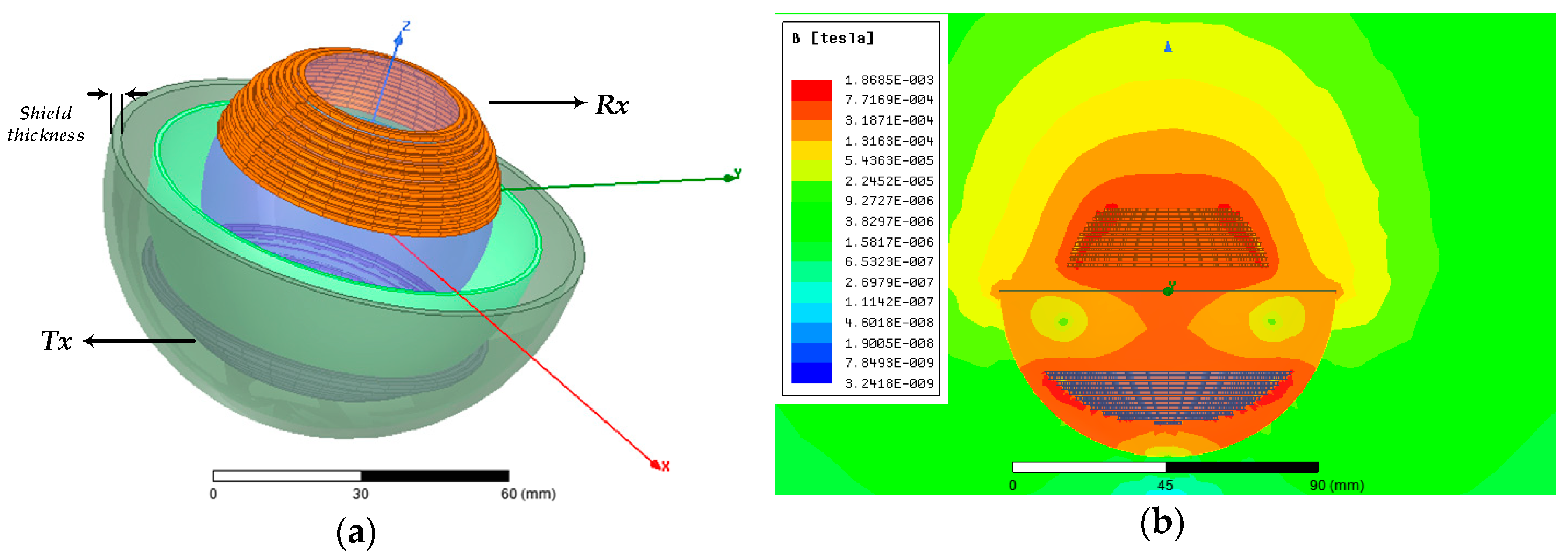
Figure 17a represents the joint WPT with an aluminum shield only for Tx. In this case, compared to Figure 13b, the leakage MF around the transmitter coil is suppressed. However, there is a high leakage MF around the receiver coil as shown in Figure 17b–d. To ensure the safety of the WPT system, the AL shield encloses both Tx and Rx as presented in Figure 18a. The magnetic field density for WPT with 0.1 mm thickness of the AL shield is illustrated in Figure 18b. In this case, the green area (outside the shielding) is 8.75 µT, which complies with ICNIRP 2010 guidelines. However, there is still leakage of MF at the right bottom side of Tx. Figure 18c shows better performance with a 0.3-mm thickness, where the heart-shaped green area is up to 5.14 µT. The thickness is increased as shown in Figure 18d. Compared to the active shielding method, the AL shield provides a reliable and practical suppression method, which takes into account the weight and size of the joint WPT. However, the induced eddy currents in the AL shield cause a slight drop in the PTE. Finally, a comparative analysis between the mitigation methods is given in Table 3.
In this paper, two mitigation methods are presented. The first is active shielding, which is not a practical solution since it requires many turns to reduce EMFs around the coils, which in turn, increases the size. In addition, it results in a low efficiency. The second is using AL shield. The simulation results proved that this method reduces EMFs to safe levels. This method can be practical for some applications, such as robotics. However, it is not a good option for human joints since there are eddy currents induced in the metallic shield, which generate heat. In this paper, we did not validate the AL shield by experiments since we attempted to find another effective mitigation method.
5. Fabrication of the WPT System and Experimental Results
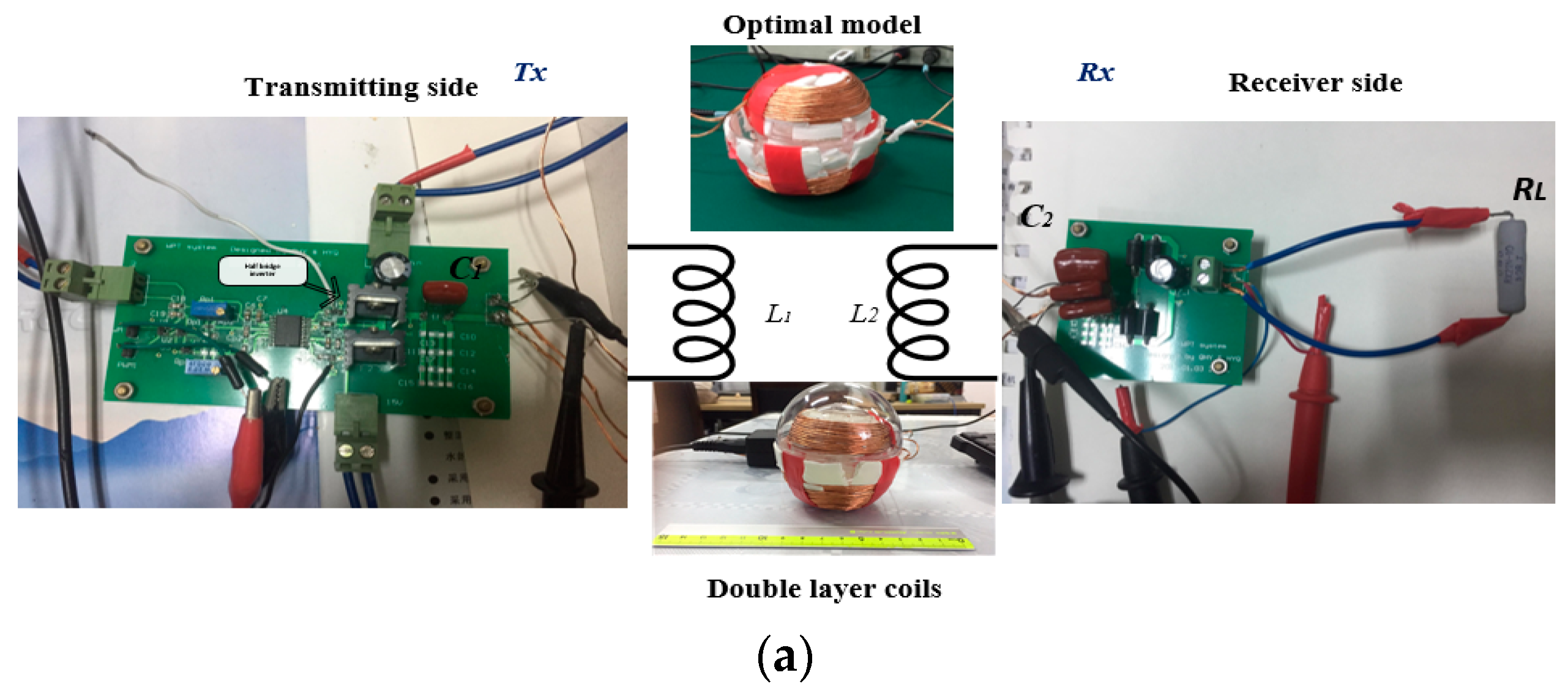
The WPT system was fabricated to validate the calculated and simulated results. A multi-strand Litz wire was used to wound the coils (reduce skin effect and losses, especially at high frequency). A half-bridge inverter on Tx side was used. To ensure there is no friction between the spherical structures, a smooth surface material should separate them. In this paper, series-series (SS) compensation topology was used, as shown in Figure 19a. The SS-compensated WPT behaves as constant current source (CCO), and the primary capacitor is constant for SS regardless of the coupling and load variation. The capacitors were changed to radio frequency (RF) mica capacitors for better performance. Two cases were assessed. The first was the double-layer windings, as shown in Figure 19b (and presented in Figure 9c). The double-layer model was chosen because it is a close case to the optimal model based on the coupling coefficient. The second was the optimal model as given in Figure 19c (and displayed in Figure 9e). Figure 19d illustrates the case of the modified hemisphere windings; this model was presented in Figure 9d, and it will be discussed in Section 5.2.
5.1. Measurements and Discussions
Two winding models were validated. The switching signals are given in Figure 20a. Figure 20b presents the input (blue) and output voltages of the optimal model at the resonant frequency (496 kHz). The measured values of L1, L2, R1, and R2 for both models are given in Table 4.
The experiments were conducted with 30-Ω load and 10-volt input voltage. The measured results are given in Table 5. The measured efficiency is DC-DC and represents the system efficiency, which is the ratio of the output power (Pout) and the total input power from the source (Pin) including the power loss in the power source and other components. On the other hand, the simulated efficiency is coil-to-coil efficiency without including any power loss.
The efficiency for both cases is illustrated in Figure 21. For the double-layer model (Figure 21a), the fluctuations of M and k will affect the performance of the WPT system. On the other hand, the performance of WPT is greatly improved in the case of the optimal model (Figure 21b). As a result, the Rx can rotate inside the Tx from 0° to 85° while maintaining high efficiency.
5.2. Measurements without Converters
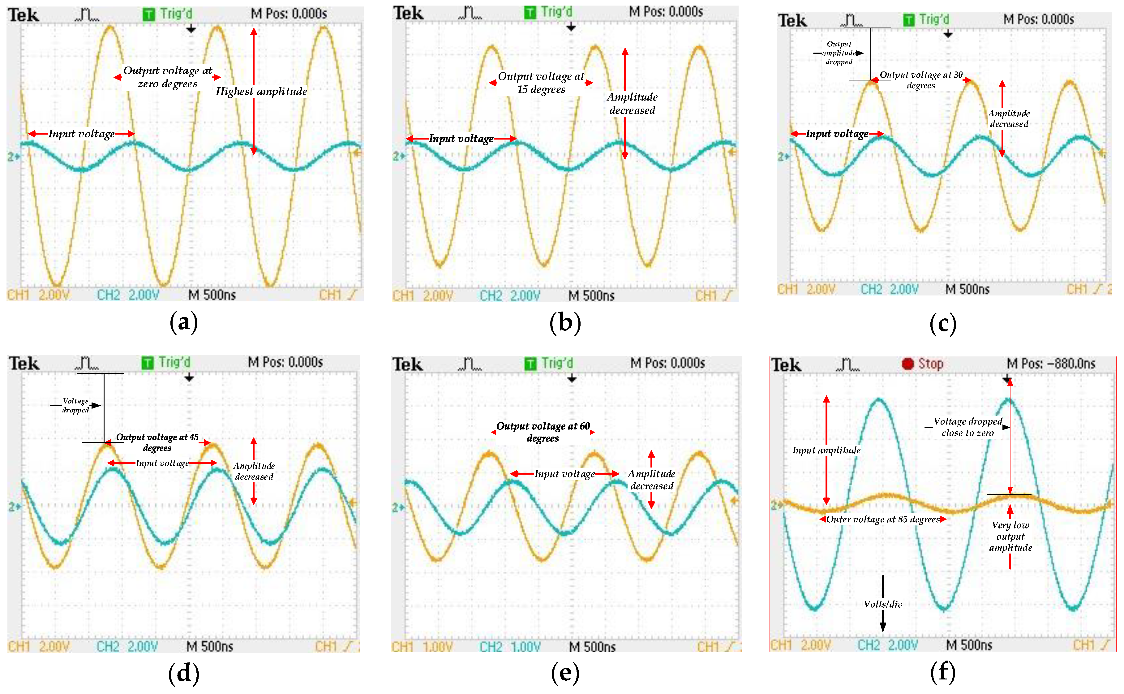
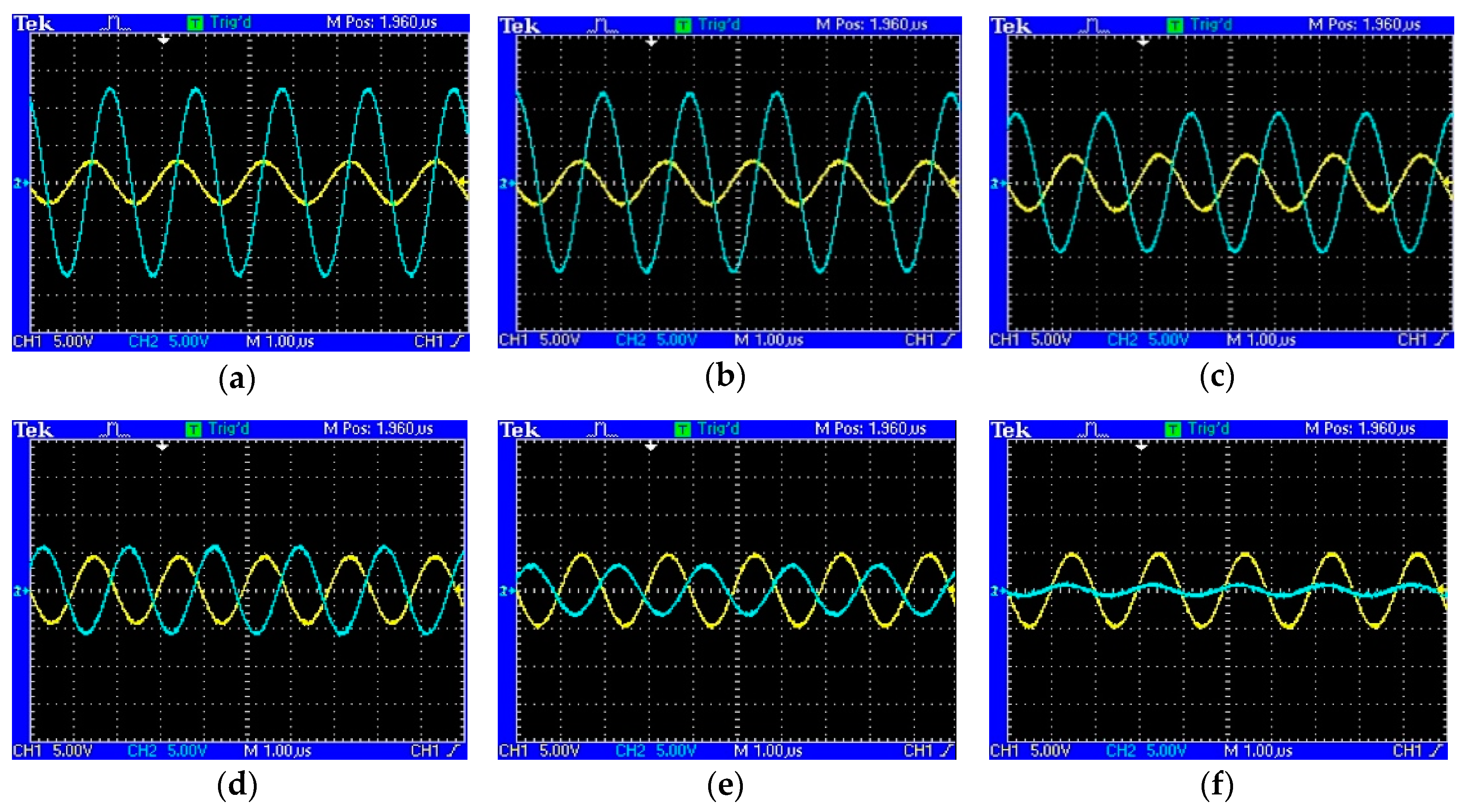
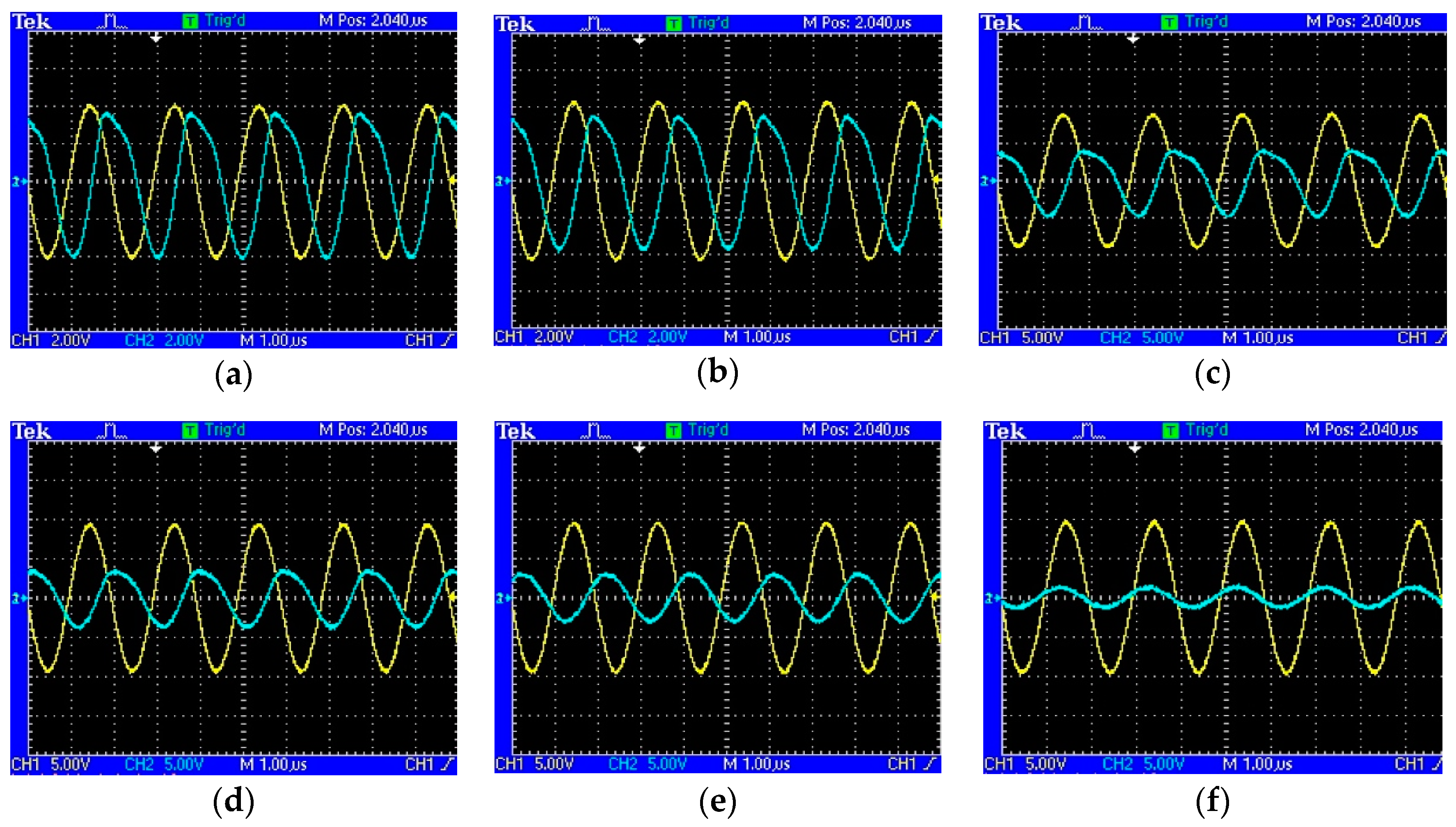
The experiments were implemented without converters (inverter and rectifier). In this study, the hemisphere, optimal models, and modified hemisphere are validated and compared by experiments. A signal generator, oscilloscope, loads, and LED lights were used. Figure 22 presents the input and output voltages of the hemisphere model under different angular misalignments at the resonant frequency of 509 kHz. At α = 85°, the output voltage will drop close to zero. On the other hand, in Figure 23 for the optimal model, the amplitude of the output voltage will be higher when α increases. At α = 85°, the output voltage drops a little. However, it maintains a high value. Figure 24 displays the input and output voltages of the optimal model with a 5-Ω load; similar to the case without load, the output voltage will increase with the angular misalignment, and at higher degrees, it will drop a little (because of the mutual inductance fluctuation as mentioned before).
As shown in Figure 10b, the fluctuation of the mutual inductance for the hemisphere windings is high (close to the case of the modified hemisphere windings), and the value of the mutual inductance will drop when α increases. This case is validated by the experiment. The input and output voltages of the modified hemisphere model (Figure 9d) are displayed in Figure 25 and Figure 26, where two types of loads were given. In Figure 25, a 5-Ω load was used. If the angle α increases, the value of the output voltage will drop and, when α = 85°, the output voltage will be close to zero. On the other hand, in Figure 26, an LED load was used. In this case, the output voltage will also drop close to zero when α becomes 85°.
5.3. Comparative Study with Other Research Works
In order to show the benefit of adopting the proposed winding method, comparison of numerical results to other relevant research works are provided. The comparative analysis should compare different studies that have similar characteristics including several aspects, for example, the size and shape of the coils, cost assessment, transferred power, and efficiency. The cost assessment of the WPT system can take into account the number of required components, such as Litz wire to wind the coils, in addition to the inverter switches, diodes, and capacitances to build the circuit. In this paper, an SS-compensated WPT system was fabricated with a half-bridge inverter. In addition, radio frequency (RF) mica-type capacitors from Cornell Dubilier Electronics (CDE) in Liberty; SC; US, were used, where each capacitor CD15FA102JO3F 1000 PF with rated voltage 100 V cost USD 4.18, and capacitor (CD15FA101JO3F) 100 PF with rated voltage 100 V cost USD 2.75. Table 6 gives a comparison between this study and other research works that have discussed the 3D-structure WPT.
6. Conclusions
In this paper, we proposed a winding method for a bio-inspired joint for a WPT system. The receiver coil is wired on a small sphere, which can rotate inside a hemispherical structure. An algorithm was designed to obtain the optimal model of the proposed winding method. Modeling and simulations of five winding methods were conducted. Moreover, the winding methods were compared based on the fluctuation of the mutual inductance and coupling coefficient when Rx rotates inside Tx. The magnetic field density was investigated in detail considering the safety issue, which is linked to the human exposure to EMFs. To ensure the safety and reliability of the proposed system, EMFs mitigation methods were proposed, and the advantages and disadvantages were given. The study proved that a 0.3 mm metallic shield of aluminum can suppress the EMFs around the coils. Magnetic field density of 5.14 µT was generated, and this value complies with the ICNIRP 2010 guidelines. Furthermore, the obtained results were validated by several experiments. Both measurement and simulation results were in good agreement. The fluctuation of the mutual inductance was reduced by the optimized model. The mutual inductance was between 3.5 µH at α = 0° and 4.5 µH at α = 85°. As a result, the efficiency can maintain a value of up to 86% at α = 85°. Finally, it is believed that this design will be useful and applicable in situations that require a wide range of angular rotation. Additional investigations will be conducted in this field, especially for designs that operate at high frequencies.
Author Contributions
Conceptualization, M.A.H. and W.C.; data curation, M.A.H.; formal analysis, M.A.H.; Investigation, M.A.H.; methodology, M.A.H. and W.C.; resources, X.Y. and W.C.; software, M.A.H.; validation, M.A.H.; writing, original draft, M.A.H.; review and editing, W.C.; supervision, X.Y.
Funding
This research received no external funding.
Conflicts of Interest
The authors declare no conflict of interest.
References
- Jiang, C.; Sun, Y.; Wang, Z.; Tang, C. Multi-load mode analysis for electric vehicle wireless supply system. Energies 2018, 11, 1925. [Google Scholar] [CrossRef]
- Zhang, H.; Lu, F.; Hofmann, H.; Liu, W.; Mi, C. A four-plate compact capacitive coupler design and LCL-compensated topology for capacitive power transfer in electric vehicle charging application. IEEE Trans. Power Electron. 2016, 31, 8541–8551. [Google Scholar]
- Yang, Y.; El Baghdadi, M.; Lan, Y.; Benomar, Y.; Van Mierlo, J.; Hegazy, O. Design methodology, modeling, and comparative study of wireless power transfer systems for electric vehicles. Energies 2018, 11, 1716. [Google Scholar] [CrossRef]
- Inoue, K.; Kusaka, K.; Itoh, J.I. Reduction in radiation noise level for inductive power transfer systems using spread spectrum techniques. IEEE Trans. Power Electron. 2018, 33, 3076–3085. [Google Scholar] [CrossRef]
- Tang, S.C.; Lun, T.L.T.; Guo, Z.; Kwok, K.W.; McDannold, N.J. Intermediate range wireless power transfer with segmented coil transmitters for implantable heart pumps. IEEE Trans. Power Electron. 2017, 32, 3844–3857. [Google Scholar] [CrossRef]
- Kang, S.H.; Choi, J.H.; Jung, C.W. Magnetic resonance wireless power transfer using three-coil system with single planar receiver for laptop applications. IEEE Trans. Consum. Electron. 2015, 61, 160–166. [Google Scholar]
- Kan, T.; Mai, R.; Mercier, P.P.; Mi, C.C. Design and analysis of a three-phase wireless charging system for lightweight autonomous underwater vehicles. IEEE Trans. Power Electron. 2017. [Google Scholar] [CrossRef]
- Sugino, M.; Kondo, H.; Takeda, S. Linear motion type transfer robot using the wireless power transfer system. In Proceedings of the 2016 International Symposium on Antennas and Propagation (ISAP), Okinawa, Japan, 24–28 October 2016; pp. 508–509. [Google Scholar]
- Vamvakas, P.; Tsiropoulou, E.E.; Vomvas, M.; Papavassiliou, S. Adaptive power management in wireless powered communication networks: A user-centric approach. In Proceedings of the IEEE 38th Sarnoff Symposium, Newark, NJ, USA, 18–20 September 2017; pp. 1–6. [Google Scholar]
- Bi, S.; Zeng, Y.; Zhang, R. Wireless powered communication networks: An overview. IEEE Wirel. Commun. 2016, 23, 10–18. [Google Scholar] [CrossRef]
- Wu, Q.; Tao, M.; Kwan Ng, D.W.; Chen, W.; Schober, R. Energy-efficient resource allocation for wireless powered communication networks. IEEE Trans. Wirel. Commun. 2016, 15, 2312–2327. [Google Scholar] [CrossRef]
- Tsiropoulou, E.E.; Mitsis, G.; Papavassiliou, S. Interest-aware energy collection & resource management in machine to machine communications. Ad Hoc Netw. 2018, 68, 48–57. [Google Scholar]
- Choi, K.W.; Aziz, A.A.; Setiawan, D.; Tran, N.M.; Ginting, L.; Kim, D.I. Distributed wireless power transfer system for internet of things devices. IEEE Internet Things J. 2018, 5, 2657–2671. [Google Scholar] [CrossRef]
- Khang, S.T.; Lee, D.J.; Hwang, I.J.; Yeo, T.D.; Yu, J.W. Microwave power transfer with optimal number of rectenna arrays for midrange applications. IEEE Antennas Wirel. Propag. Lett. 2018, 17, 155–159. [Google Scholar] [CrossRef]
- De Santi, C.; Meneghini, M.; Caria, A.; Dogmus, E.; Zegaoui, M.; Medjdoub, F.; Kalinic, B.; Cesca, T.; Zanoni, E. GaN-based laser wireless power transfer system. Materials 2018, 11, 153. [Google Scholar] [CrossRef]
- Li, Q.; Deng, Z.; Zhang, K.; Wang, B. Precise attitude control of multirotary-joint solar-power satellite. J. Guid. Control Dyn. 2018, 41, 1435–1442. [Google Scholar] [CrossRef]
- Kim, J.; Kim, D.H.; Choi, J.; Kim, K.H.; Park, Y.J. Free-positioning wireless charging system for small electronic devices using a bowl-shaped transmitting coil. IEEE Trans. Microw. Theory Tech. 2015, 63, 791–800. [Google Scholar] [CrossRef]
- Mei, H.; Thackston, K.A.; Bercich, R.A.; Jefferys, J.G.R.; Irazoqui, P.P. Cavity resonator wireless power transfer system for freely moving animal experiments. IEEE Trans. Biomed. Eng. 2017, 64, 775–785. [Google Scholar] [CrossRef] [PubMed]
- Kuo, R.C.; Riehl, P.; Satyamoorthy, A.; Plumb, W.; Tustin, P.; Lin, J. A 3D resonant wireless charger for a wearable device and a mobile phone. In Proceedings of the 2015 IEEE Wireless Power Transfer Conference (WPTC), Boulder, CO, USA, 13–15 May 2015. [Google Scholar] [CrossRef]
- Chabalko, M.J.; Sample, A.P. Three-dimensional charging via multimode resonant cavity enabled wireless power transfer. IEEE Trans. Power Electron. 2015, 30, 6163–6173. [Google Scholar] [CrossRef]
- Jeong, I.S.; Jung, B.I.; You, D.S.; Choi, H.S. Analysis of S-parameters in magnetic resonance WPT using superconducting coils. IEEE Trans. Appl. Supercond. 2016, 26, 1–4. [Google Scholar] [CrossRef]
- Lin, D.; Zhang, C.; Hui, S.Y.R. Mathematic analysis of omnidirectional wireless power transfer—Part-II three-dimensional systems. IEEE Trans. Power Electron. 2017, 32, 613–624. [Google Scholar] [CrossRef]
- Ye, Z.; Sun, Y.; Liu, X.; Wang, P.; Tang, C.; Tian, H. Power transfer efficiency analysis for omnidirectional wireless power transfer system using three-phase-shifted drive. Energies 2018, 11, 2159. [Google Scholar] [CrossRef]
- Fu, X.; Liu, F.; Chen, X. Optimization of coils for a three-phase magnetically coupled resonant wireless power transfer system oriented by the zero-voltage-switching range. In Proceedings of the Applied Power Electronics Conference and Exposition (APEC), Tampa, FL, USA, 26–30 March 2017; pp. 3708–3713. [Google Scholar]
- Kim, M.; Kim, H.; Kim, D.; Jeong, Y.; Park, H.H.; Ahn, S. A three-phase wireless-power-transfer system for online electric vehicles with reduction of leakage magnetic fields. IEEE Trans. Microw. Theory Tech. 2015, 63, 3806–3813. [Google Scholar] [CrossRef]
- Luo, Z.; Wei, X. Analysis of square and circular planar spiral coils in wireless power transfer system for electric vehicles. IEEE Trans. Ind. Electron. 2018, 65, 331–341. [Google Scholar] [CrossRef]
- Park, C.; Lee, S.; Cho, G.H.; Rim, C.T. Innovative 5-m-off-distance inductive power transfer systems with optimally shaped dipole coils. IEEE Trans. Power Electron. 2015, 30, 817–827. [Google Scholar] [CrossRef]
- Hekal, S.; Abdel-Rahman, A.B.; Jia, H.; Allam, A.; Barakat, A.; Pokharel, R.K. A novel technique for compact size wireless power transfer applications using defected ground structures. IEEE Trans. Microw. Theory Tech. 2017, 65, 591–599. [Google Scholar] [CrossRef]
- Sis, S.A.; Orta, E. A cross-shape coil structure for use in wireless power applications. Energies 2018, 11, 1094. [Google Scholar] [CrossRef]
- Liu, Z.; Chen, Z.; Li, J.; Guo, Y.; Xu, B. A Planar L-Shape Transmitter for a Wireless Power Transfer System. IEEE Antennas Wirel. Propag. Lett. 2017, 16, 960–963. [Google Scholar] [CrossRef]
- Abou Houran, M.; Yang, X.; Chen, W. Magnetically coupled resonance WPT: review of compensation topologies, resonator structures with misalignment, and EMI diagnostics. Electronics 2018, 7, 296. [Google Scholar] [CrossRef]
- Liu, D.; Hu, H.; Georgakopoulos, S.V. Misalignment sensitivity of strongly coupled wireless power transfer systems. IEEE Trans. Power Electron. 2016, 32, 5509–5519. [Google Scholar] [CrossRef]
- Liu, F.; Yang, Y.; Jiang, D.; Ruan, X.; Chen, X. Modeling and optimization of magnetically coupled resonant wireless power transfer system with varying spatial scales. IEEE Trans. Power Electron. 2017, 32, 3240–3250. [Google Scholar] [CrossRef]
- Samanta, S.; Rathore, A.K. A New Current-Fed CLC Transmitter and LC receiver topology for inductive wireless power transfer application: analysis, design, and experimental results. IEEE Trans. Transp. Electrif. 2015, 1, 357–368. [Google Scholar] [CrossRef]
- Zhang, C.; Lin, D.; Hui, S.R. Ball-joint wireless power transfer systems. IEEE Trans. Power Electron. 2018, 33, 65–72. [Google Scholar] [CrossRef]
- Tanabe, F.; Yoshimoto, S.; Noda, Y.; Araki, T.; Uemura, T.; Takeuchi, Y.; Imai, M.; Sekitani, T. Flexible sensor sheet for real-time pressure monitoring in artificial knee joint during total knee arthroplasty. In Proceedings of the 39th Annual International Conference of the IEEE Engineering in Medicine and Biology Society (EMBC), Seogwipo, Korea, 11–15 July 2017. [Google Scholar]
- Qiu, Y.; Li, K.M.; Neoh, E.C.; Zhang, H.; Khaw, X.Y.; Fan, X.; Miao, C. Fun-Knee™: A novel smart knee sleeve for Total-Knee-Replacement rehabilitation with gamification. In Proceedings of the IEEE 5th International Conference on Serious Games and Applications for Health (SeGAH), Perth, Australia, 2–4 April 2017. [Google Scholar] [CrossRef]
- Abou Houran, M.; Yang, X.; Chen, W.; Samizadeh, M. Wireless power transfer: critical review of related standards. In Proceedings of the 2018 International Power Electronics Conference (ECCE Asia), Niigata, Japan, 20–24 May 2018; pp. 1062–1066. [Google Scholar]
- Narayanamoorthi, R.; Juliet, A.V. IoT enabled home cage with three dimensional resonant wireless power and data transfer scheme for freely moving animal. IEEE Sens. J. 2018, 18, 8154–8161. [Google Scholar] [CrossRef]
Figure 1.
Wireless power transfer (WPT) classifications.

Figure 2.
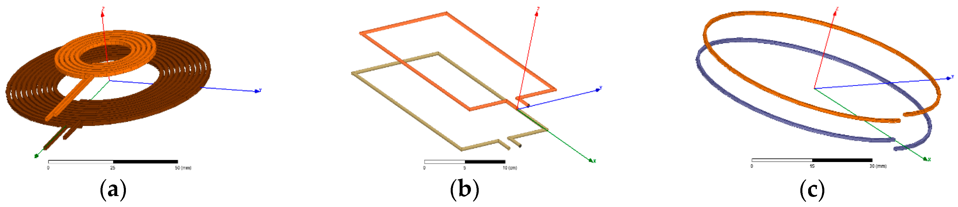
Some WPT coil structures (designed by Ansys Maxwell 3D, Canonsburg, PA, USA; 2018): (a) circular spiral coils; (b) rectangular coils; (c) circular coils; (d) planar spiral coils; (e) helical coils; (f) square coils; (g) hexagon coils; (h) conical coils.
Figure 2.
Some WPT coil structures (designed by Ansys Maxwell 3D, Canonsburg, PA, USA; 2018): (a) circular spiral coils; (b) rectangular coils; (c) circular coils; (d) planar spiral coils; (e) helical coils; (f) square coils; (g) hexagon coils; (h) conical coils.

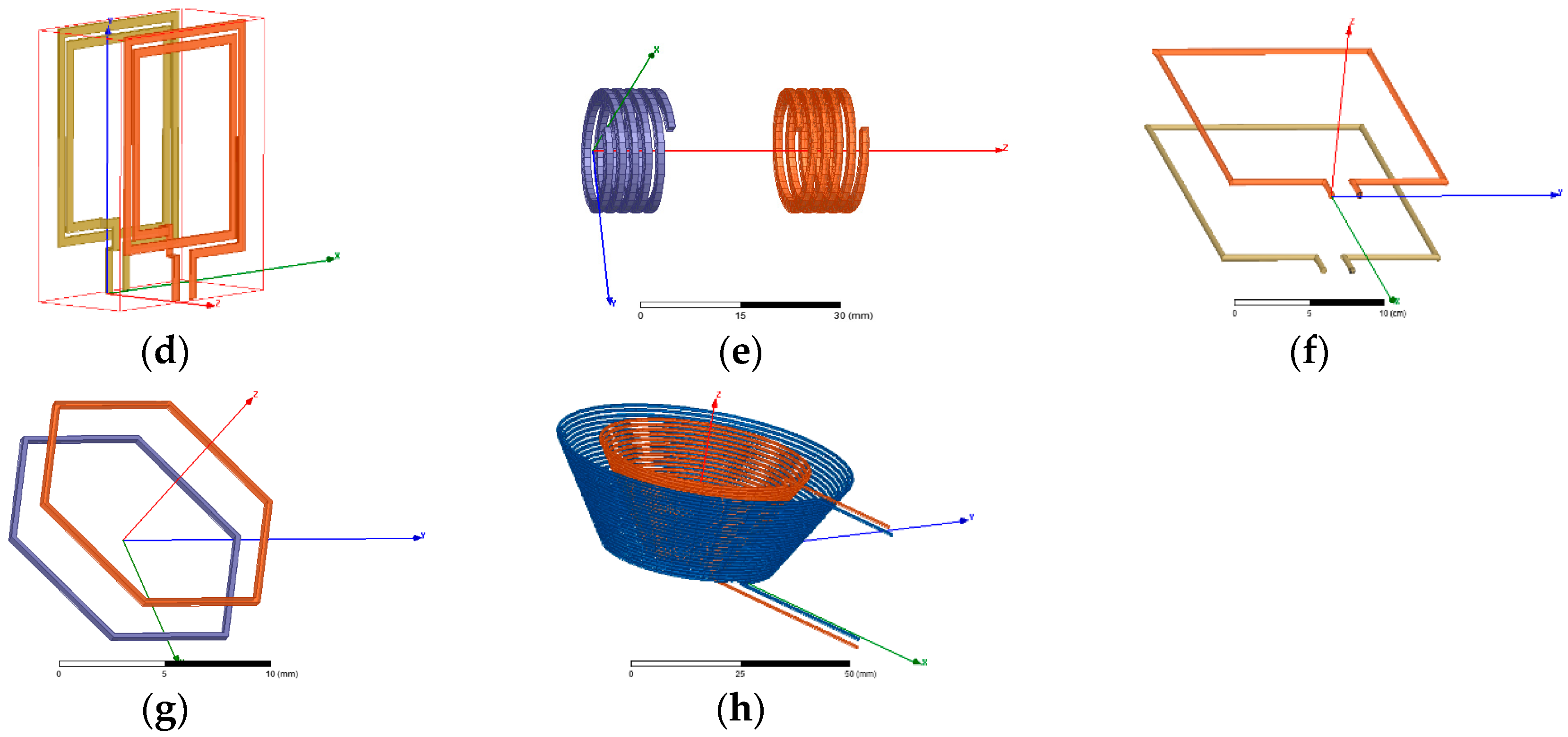
Figure 3.
Modeling of the spherical-joint system: (a) spherical structure with small sphere (orange) and large sphere; (b) view of the joint system under different angular misalignment α (0–85°); (c) dimensions of the studied joint structure.
Figure 3.
Modeling of the spherical-joint system: (a) spherical structure with small sphere (orange) and large sphere; (b) view of the joint system under different angular misalignment α (0–85°); (c) dimensions of the studied joint structure.

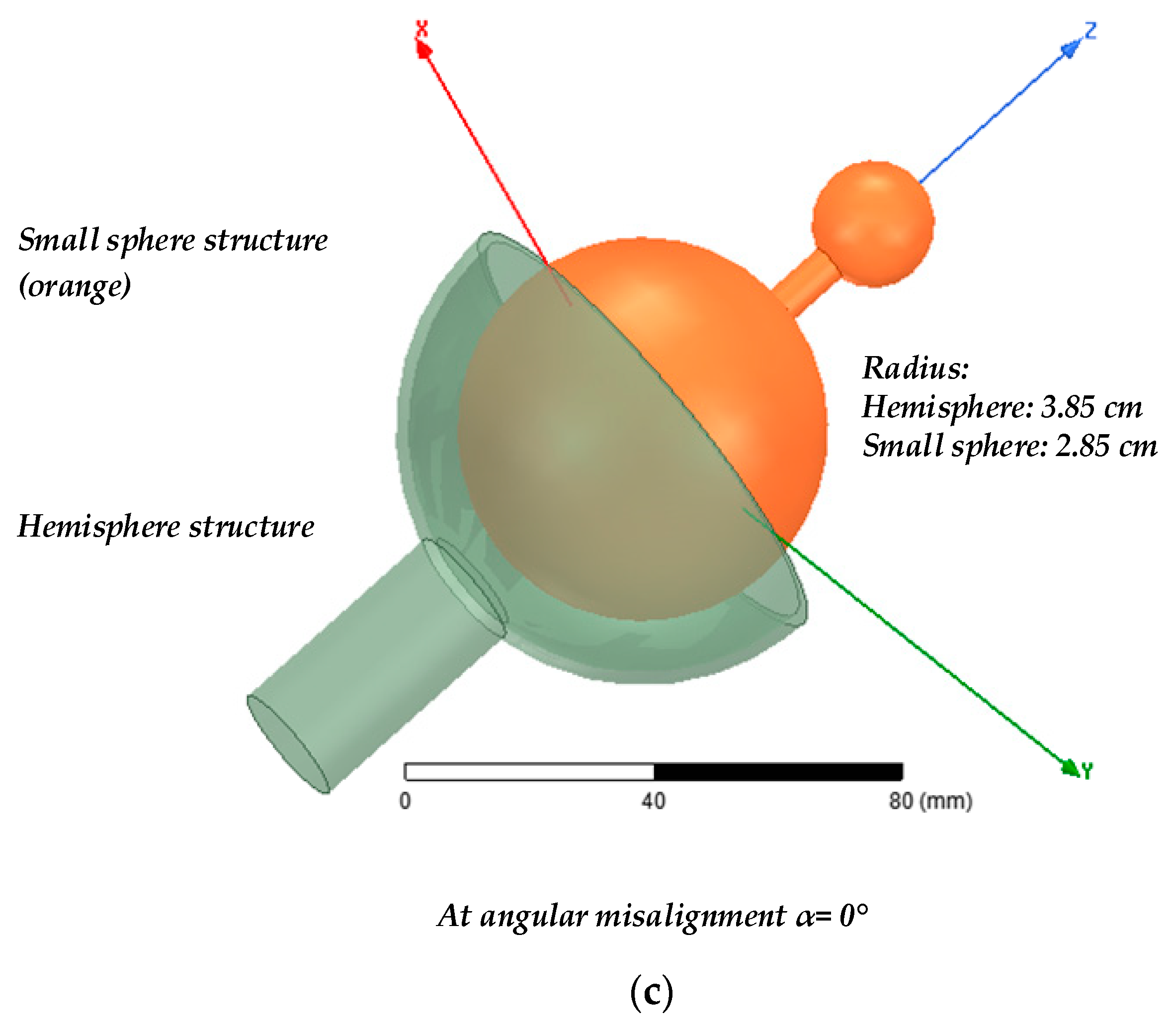
Figure 4.
Basic winding methods for the transmitter coil: Cases (A–D) cover the hemisphere; case (E) covers the middle area (equator winding).
Figure 4.
Basic winding methods for the transmitter coil: Cases (A–D) cover the hemisphere; case (E) covers the middle area (equator winding).

Figure 5.
Basic winding methods for the receiving coil, where Rx winding can cover the whole sphere. Cases (a1–d1) cover the upper hemisphere of the small sphere, case (e) covers the middle area, and cases (a2–d2) cover the lower hemisphere of the small sphere.
Figure 5.
Basic winding methods for the receiving coil, where Rx winding can cover the whole sphere. Cases (a1–d1) cover the upper hemisphere of the small sphere, case (e) covers the middle area, and cases (a2–d2) cover the lower hemisphere of the small sphere.

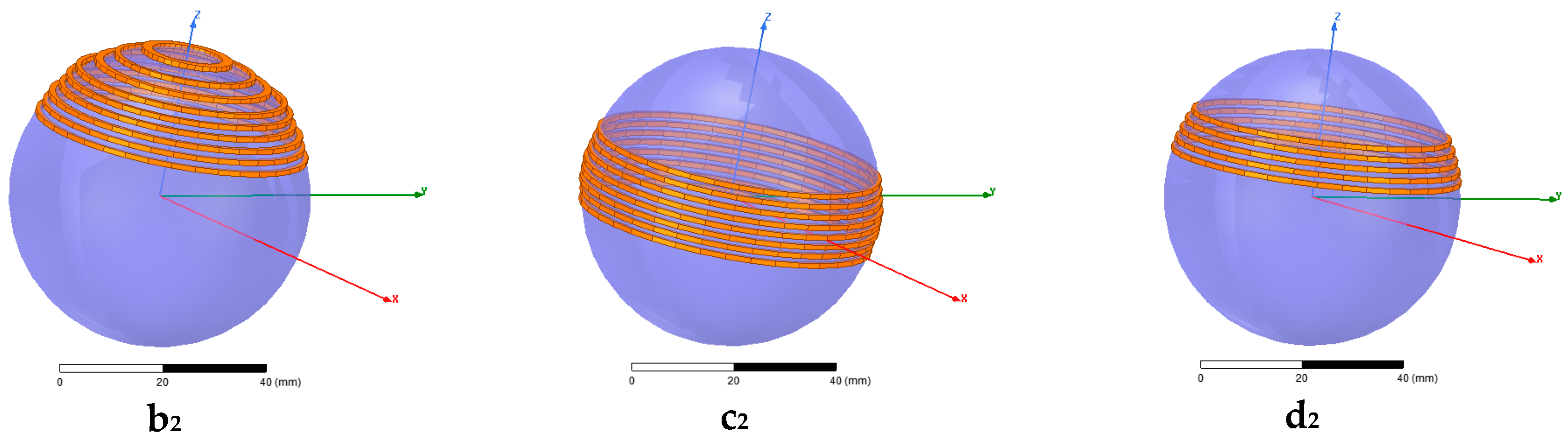
Figure 6.
Joint–WPT system in the y-z plane with several variables.

Figure 7.
Flowchart representing the algorithm design of the joint WPT.

Figure 8.
WPT system: (a) magnetically coupled resonance WPT (MCR WPT); (b) the equivalent circuit of series–series (SS)-compensated WPT.
Figure 8.
WPT system: (a) magnetically coupled resonance WPT (MCR WPT); (b) the equivalent circuit of series–series (SS)-compensated WPT.
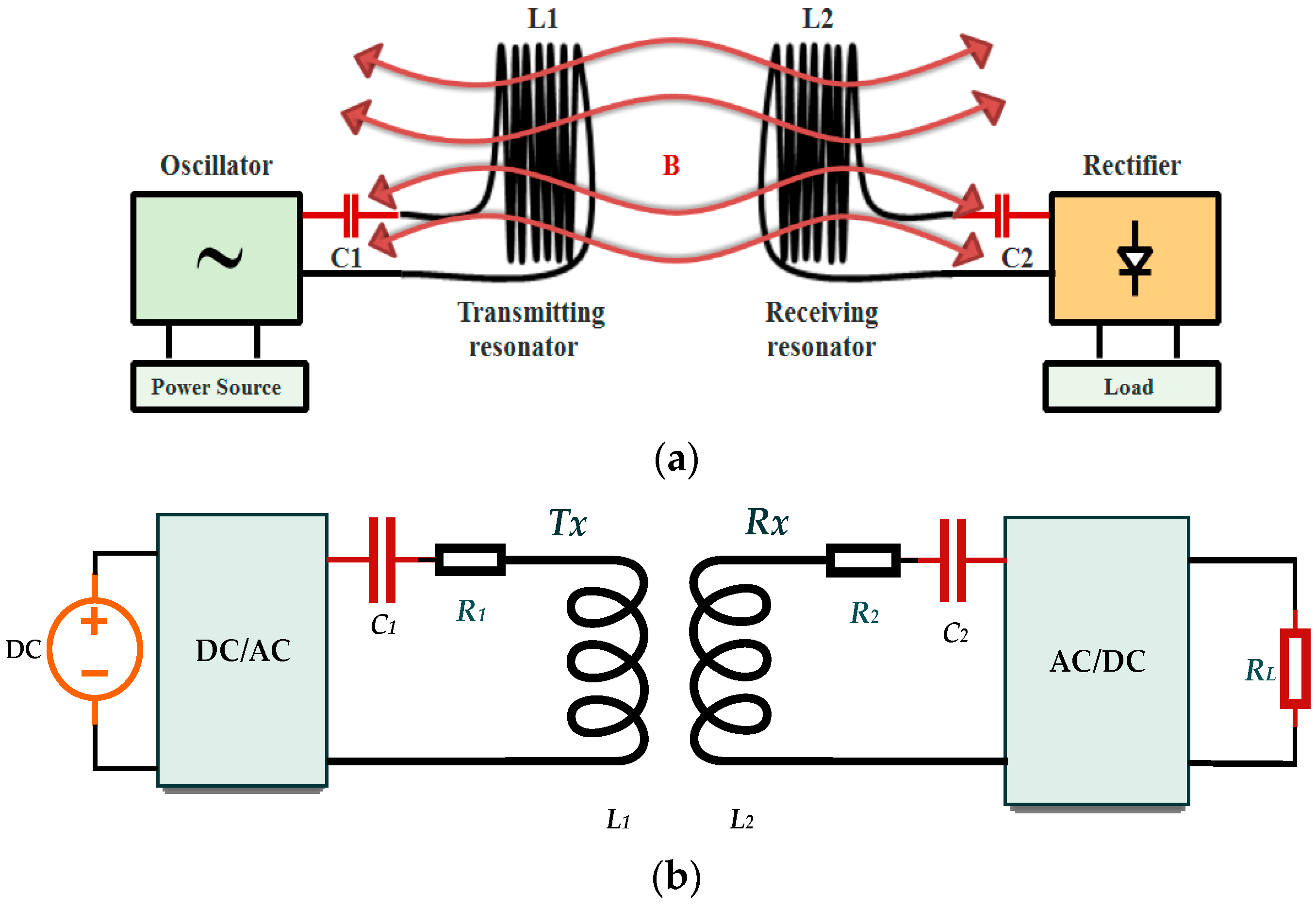
Figure 9.
Some solutions of the optimization process: (a) equator windings; (b) hemisphere windings; (c) double-layer windings; (d) modified hemisphere windings; (e) optimal model.
Figure 9.
Some solutions of the optimization process: (a) equator windings; (b) hemisphere windings; (c) double-layer windings; (d) modified hemisphere windings; (e) optimal model.

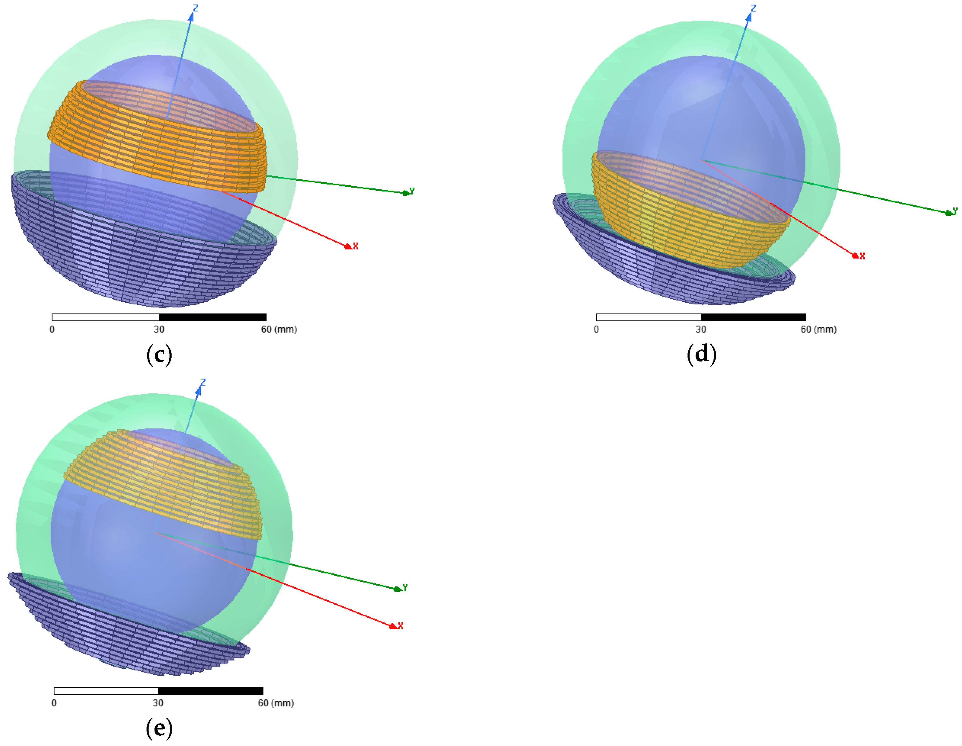
Figure 10.
The mutual inductance and coupling coefficient: (a) equator windings; (b) hemisphere windings; (c) double-layer windings; (d) optimal model.
Figure 10.
The mutual inductance and coupling coefficient: (a) equator windings; (b) hemisphere windings; (c) double-layer windings; (d) optimal model.
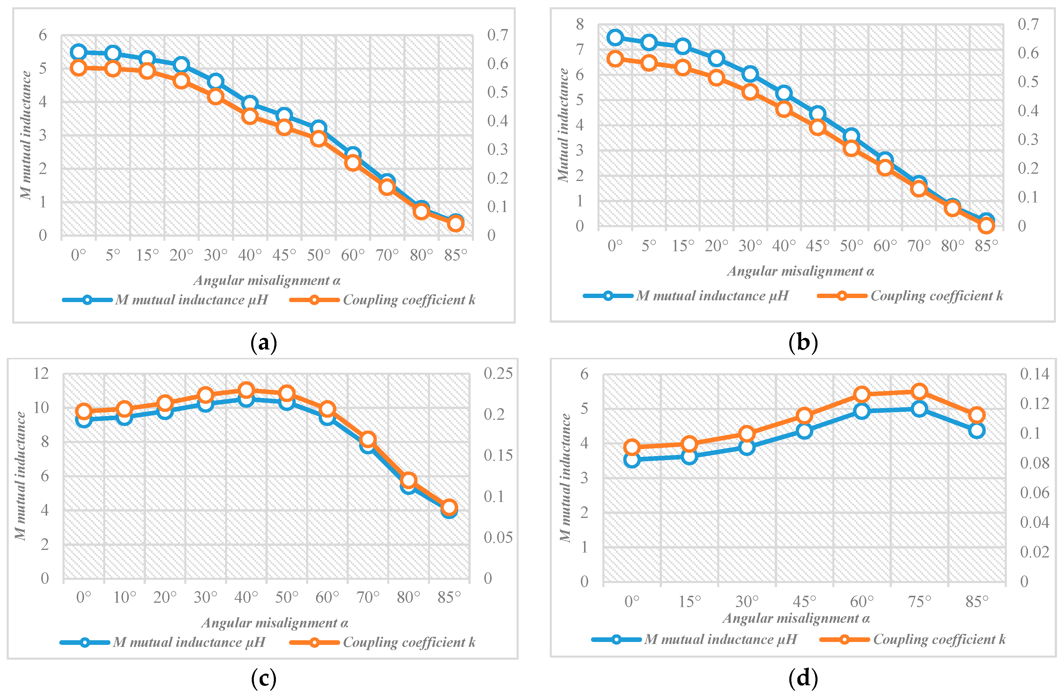
Figure 11.
The relationship between efficiency, load, and angular misalignment: (a) equator windings; (b) hemisphere windings; (c) optimal model; (d) output power of the optimal model.
Figure 11.
The relationship between efficiency, load, and angular misalignment: (a) equator windings; (b) hemisphere windings; (c) optimal model; (d) output power of the optimal model.


Figure 12.
The relationship between efficiency, load, and resonant frequency: (a) equator windings; (b) hemisphere windings; (c) double layer windings; (d) modified hemisphere windings; (e) optimal model.
Figure 12.
The relationship between efficiency, load, and resonant frequency: (a) equator windings; (b) hemisphere windings; (c) double layer windings; (d) modified hemisphere windings; (e) optimal model.

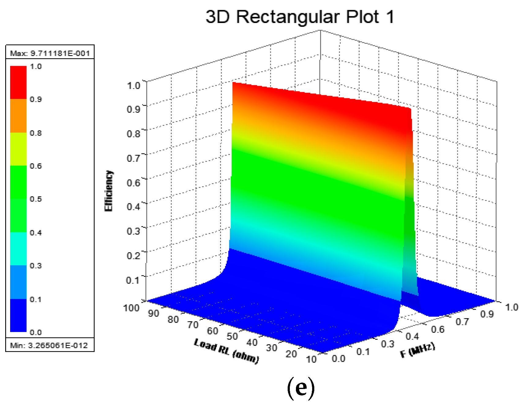
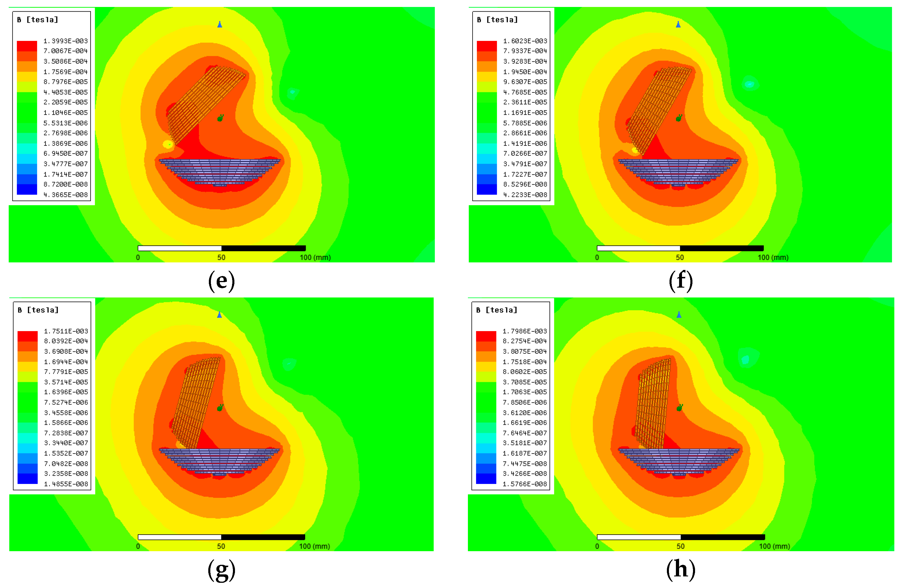
Figure 13.
The magnetic field density of the optimal model at different angular misalignments: (a) magnetization direction; (b) α = 0°; (c) α = 15°; (d) α = 30°; (e) α = 45°; (f) α = 60°; (g) α = 75°; (h) α = 85°.
Figure 13.
The magnetic field density of the optimal model at different angular misalignments: (a) magnetization direction; (b) α = 0°; (c) α = 15°; (d) α = 30°; (e) α = 45°; (f) α = 60°; (g) α = 75°; (h) α = 85°.


Figure 14.
The magnetic field density: (a) equator windings; (b) hemisphere windings; (c) double-layer windings; (d) modified hemisphere windings.
Figure 14.
The magnetic field density: (a) equator windings; (b) hemisphere windings; (c) double-layer windings; (d) modified hemisphere windings.

Figure 15.
The WPT system: (a) shielding coils for Tx and Rx (in green); (b) current direction in the shielding turns (in green).
Figure 15.
The WPT system: (a) shielding coils for Tx and Rx (in green); (b) current direction in the shielding turns (in green).

Figure 16.
The magnetic field density and efficiency at 50-Ω load: (a) without shielding coils; (b) efficiency without shielding coils; (c) shield coils are part of Tx and Rx; (d) efficiency when shielding coils are part of Tx and Rx; (e) shielding coils are separated from Tx and Rx; (f) efficiency when the shielding coils are separated from Tx and Rx.
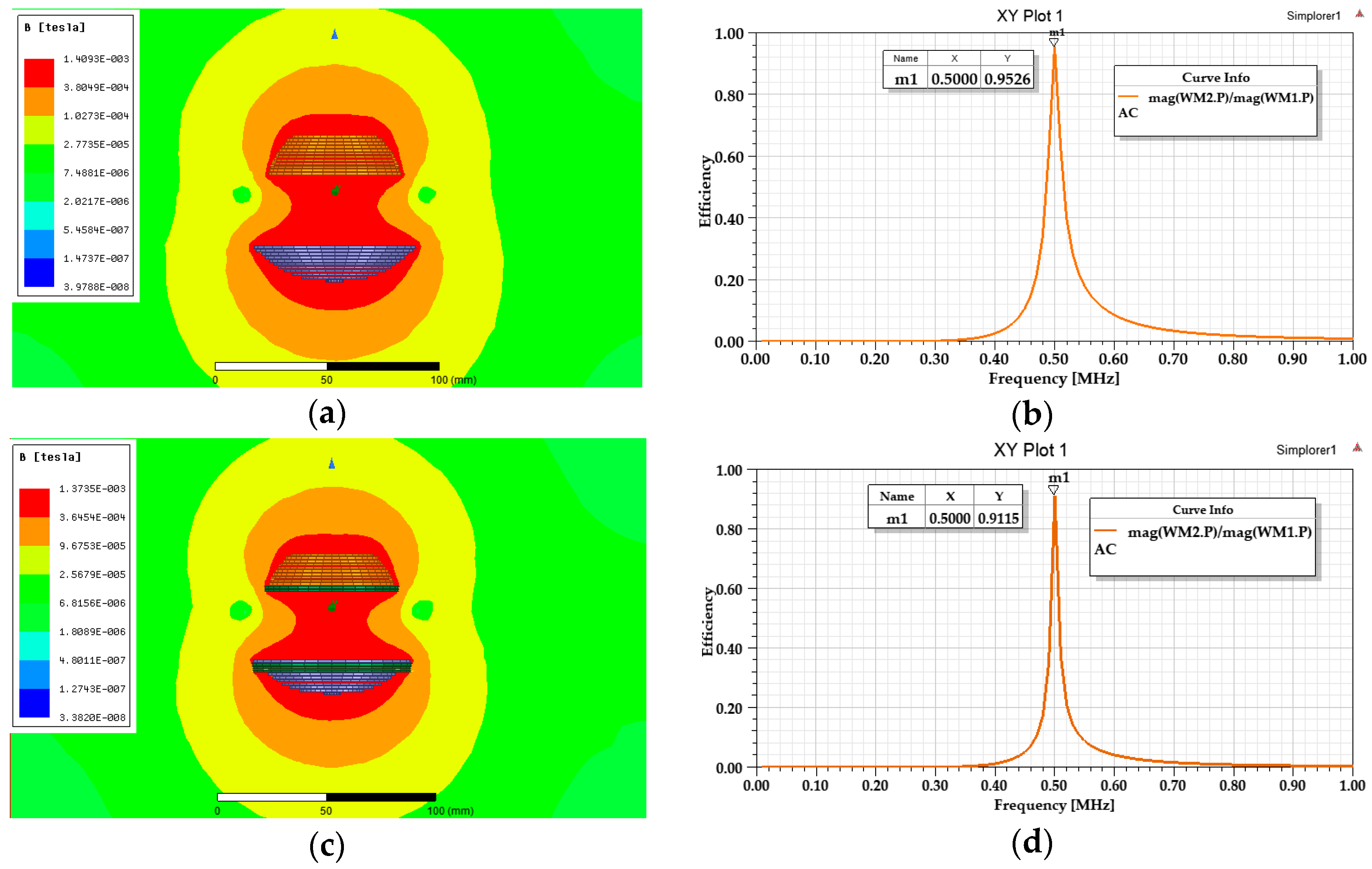

Figure 17.
Joint–WPT system: (a) aluminum sheet (AL shield) for Tx only; (b) 0.3-mm AL shield; (c) 1-mm AL shield; (d) 2-mm AL shield.
Figure 17.
Joint–WPT system: (a) aluminum sheet (AL shield) for Tx only; (b) 0.3-mm AL shield; (c) 1-mm AL shield; (d) 2-mm AL shield.


Figure 18.
The joint–WPT system with shielding and magnetic field density: (a) AL shield for Tx and Rx; (b) 0.1–mm AL shield; (c) 0.3–mm AL shield; (d) 0.5–mm AL shield.
Figure 18.
The joint–WPT system with shielding and magnetic field density: (a) AL shield for Tx and Rx; (b) 0.1–mm AL shield; (c) 0.3–mm AL shield; (d) 0.5–mm AL shield.

Figure 19.
The WPT system: (a) SS-compensated WPT; (b) double-layer windings; (c) optimal model; (d) modified hemisphere windings.
Figure 19.
The WPT system: (a) SS-compensated WPT; (b) double-layer windings; (c) optimal model; (d) modified hemisphere windings.

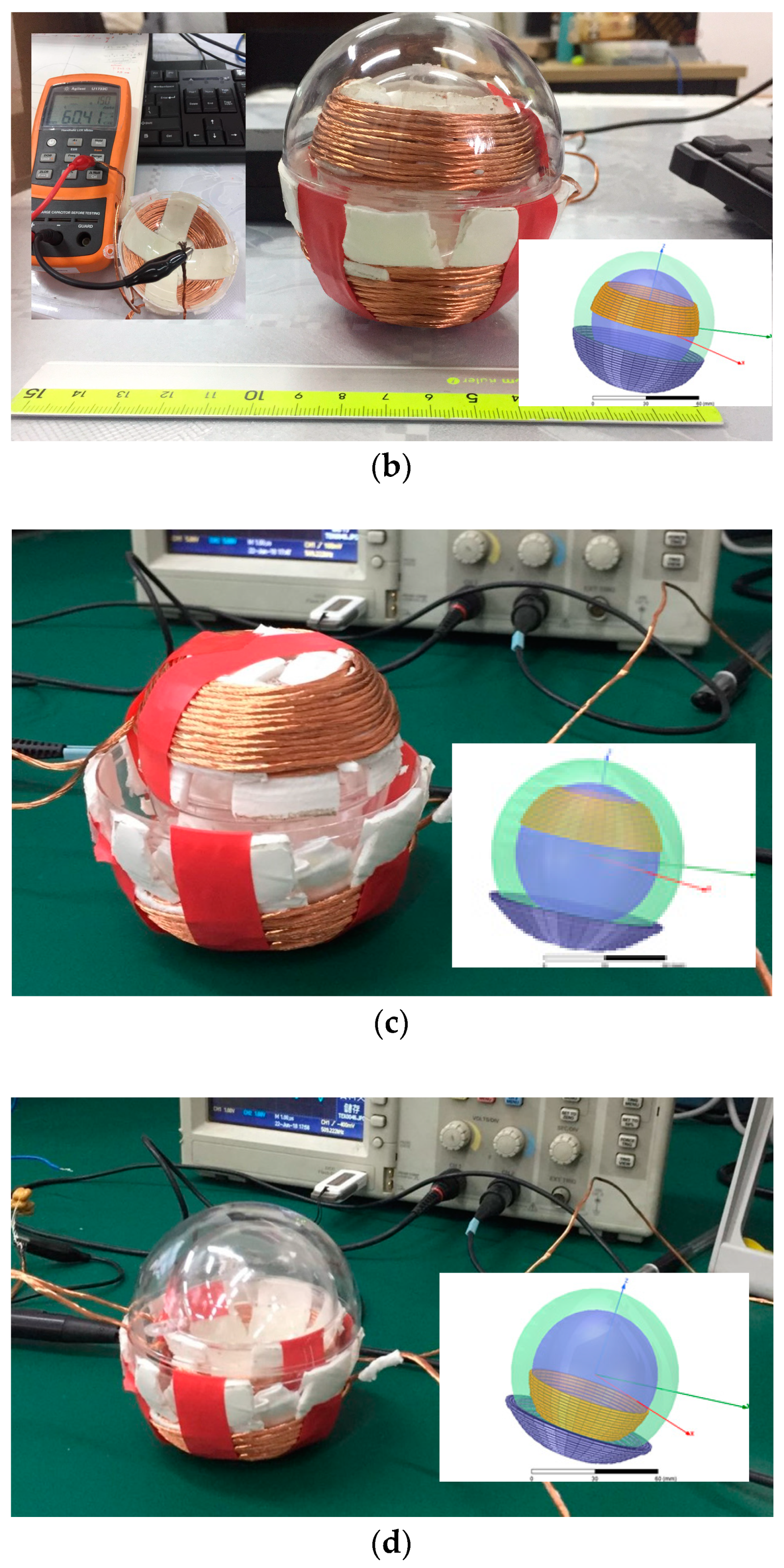
Figure 20.
(a) Pulse-width modulation (PWM) signals; (b) input and output (orange) voltages for the optimal model at α = 0°.
Figure 20.
(a) Pulse-width modulation (PWM) signals; (b) input and output (orange) voltages for the optimal model at α = 0°.
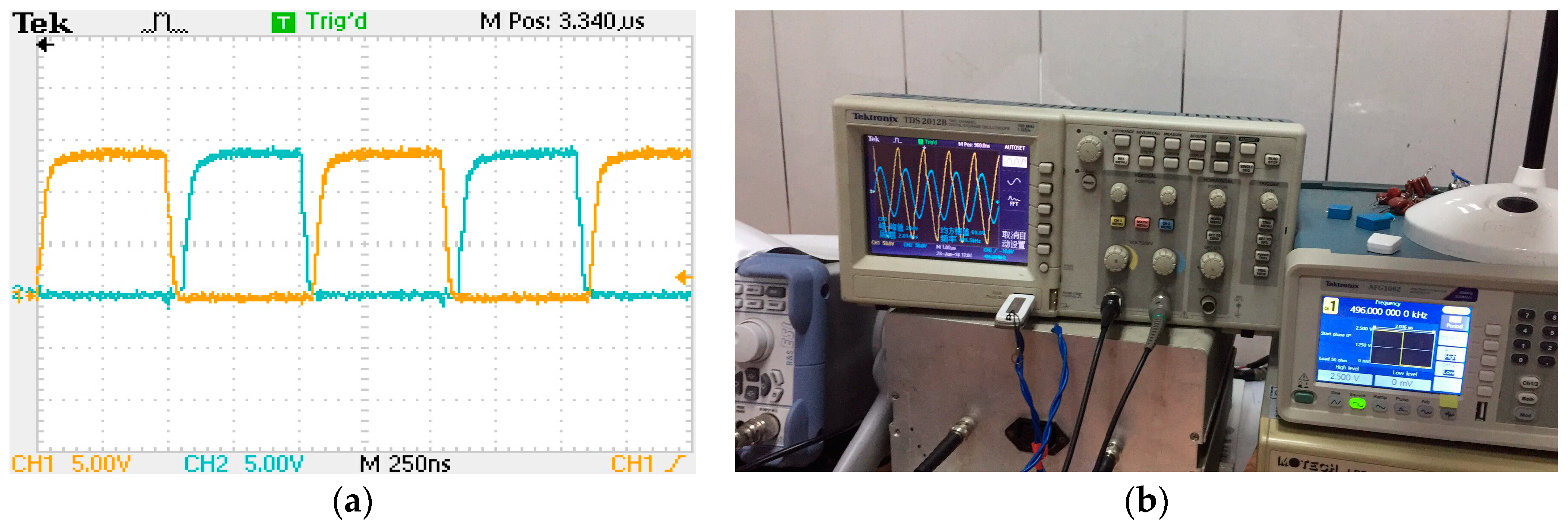
Figure 21.
Efficiency: (a) double-layer windings; (b) optimal model.
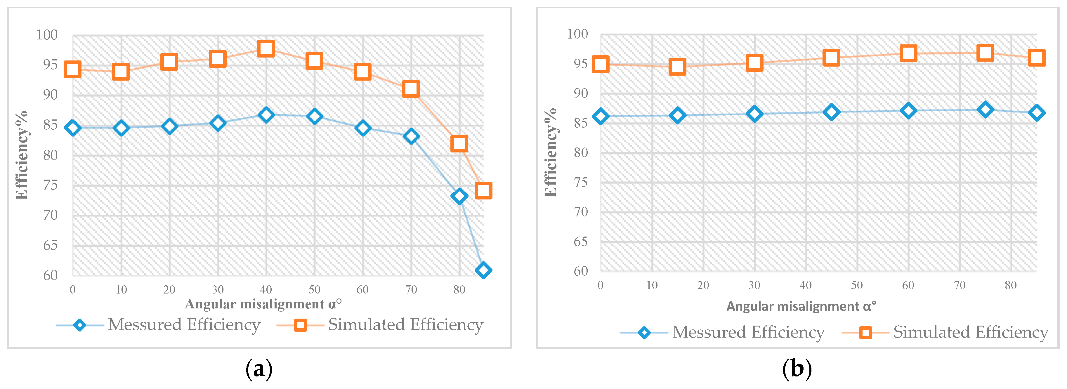
Figure 22.
Input (blue) and output (orange) coil-to-coil voltages for the hemisphere windings: (a) α = 0°; (b) α = 15°; (c) α = 30°; (d) α = 45°; (e) α = 60°; (f) α = 85°.
Figure 22.
Input (blue) and output (orange) coil-to-coil voltages for the hemisphere windings: (a) α = 0°; (b) α = 15°; (c) α = 30°; (d) α = 45°; (e) α = 60°; (f) α = 85°.

Figure 23.
Input (blue) and output (orange) coil-to-coil voltages for the optimized model: (a) α = 0°; (b) α = 15°; (c) α = 30°; (d) α = 45°; (e) α = 60°; (f) α = 85°.
Figure 23.
Input (blue) and output (orange) coil-to-coil voltages for the optimized model: (a) α = 0°; (b) α = 15°; (c) α = 30°; (d) α = 45°; (e) α = 60°; (f) α = 85°.
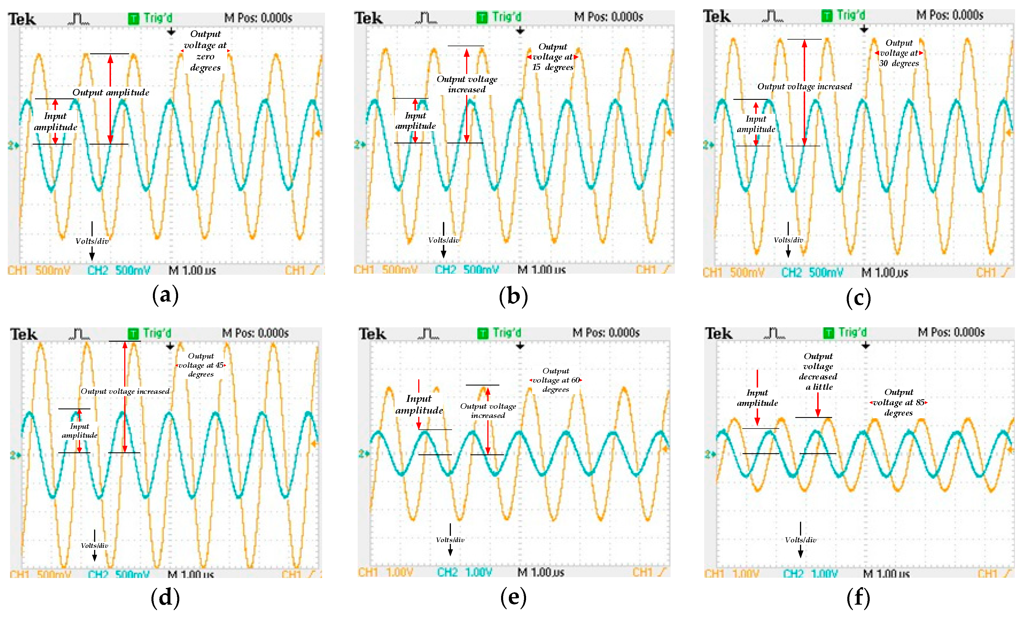
Figure 24.
Input (yellow) and output (blue) coil-to-coil voltages for the optimized model with 5-Ω load: (a) α = 0°; (b) α = 15°; (c) α = 30°; (d) α = 45°; (e) α = 60°; (f) α = 85°.
Figure 24.
Input (yellow) and output (blue) coil-to-coil voltages for the optimized model with 5-Ω load: (a) α = 0°; (b) α = 15°; (c) α = 30°; (d) α = 45°; (e) α = 60°; (f) α = 85°.
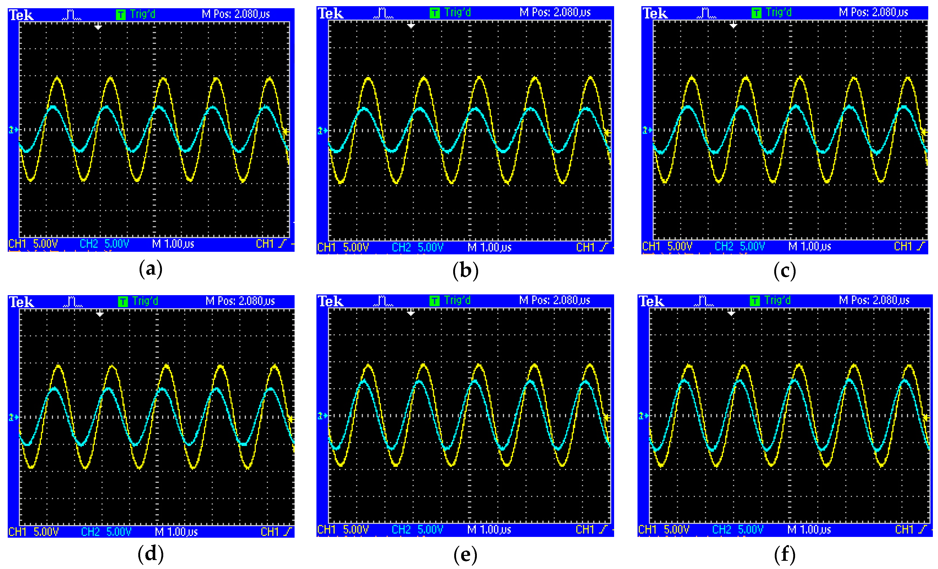
Figure 25.
Input (yellow) and output (blue) coil-to-coil voltages for the modified hemisphere model with 5-Ω load: (a) α = 0°; (b) α = 15°; (c) α = 30°; (d) α = 45°; (e) α = 60°; (f) α = 85°.
Figure 25.
Input (yellow) and output (blue) coil-to-coil voltages for the modified hemisphere model with 5-Ω load: (a) α = 0°; (b) α = 15°; (c) α = 30°; (d) α = 45°; (e) α = 60°; (f) α = 85°.

Figure 26.
Input (yellow) and output (blue) voltages for the modified hemisphere model with an LED load (V (RMS) = 7.034 V): (a) α = 0°; (b) α = 15°; (c) α = 30°; (d) α = 45°; (e) α = 60°; (f) α = 85°.
Figure 26.
Input (yellow) and output (blue) voltages for the modified hemisphere model with an LED load (V (RMS) = 7.034 V): (a) α = 0°; (b) α = 15°; (c) α = 30°; (d) α = 45°; (e) α = 60°; (f) α = 85°.


Table 1.
Combination methods of the transmitter and receiver winding methods.
| Case | a1 | b1 | c1 | d1 | e | a2 | b2 | c2 | d2 |
|---|---|---|---|---|---|---|---|---|---|
| A | Aa1 | Ab1 | Ac1 | Ad1 | Ae | Aa2 | Ab2 | Ac2 | Ad2 |
| B | Ba1 | Bb1 | Bc1 | Bd1 | Be | Ba2 | Bb2 | Bc2 | Bd2 |
| C | Ca1 | Cb1 | Cc1 | Cd1 | Ce | Ca2 | Cb2 | Cc2 | Cd2 |
| D | Da1 | Db1 | Dc1 | Dd1 | De | Da2 | Db2 | Dc2 | Dd2 |
| E | Ea1 | Eb1 | Ec1 | Ed1 | Ee | Ea2 | Eb2 | Ec2 | Ed2 |
Table 2.
Parameters of case studies.
| WPT | f0 | Number of Turns N1/N2 | Inductances L1/L2 µH | Mutual Inductance M µH, at α = 0° | Coupling Coefficient k at α = 0° | C1/C2 nF |
|---|---|---|---|---|---|---|
| Equator windings (single layer) | 500 kHz | 20/17 | 28.971/14.25 | 12.27 | 0.604 | 7.1/3.49 |
| Hemisphere windings (single layer) | 21/16 | 21.14/7.8156 | 7.478 | 0.58177 | 4.793/12.96 | |
| Double-layer windings | 34/22 | 60.71/34.25 | 9.31 | 0.204 | 1.66/3 | |
| Modified Hemisphere windings (multi-layer) | 34/24 | 50.08/29.57 | 17.842 | 0.463 | 2/3.4 | |
| Optimal model | 34/24 | 50.699/29.88 | 3.6117 | 0.089 | 2/3.4 |
Table 3.
A comparative analysis between EMF suppression methods.
| Suppression Methods | N1/N2 and Thickness | Inductances L1/L2 µH | M µH (α = 0°) | k at α = 0° | C1/C2 nF (at 500 kHz) | Efficiency at 50 Ω | Advantages/Disadvantages |
|---|---|---|---|---|---|---|---|
| Optimal model without shield | 34/24 | 50.699/29.88 | 3.6117 | 0.089 | 2/3.4 | 95.26% | Unsafe EMFs in the coil’s vicinities. |
| Active shielding (shielding coils are part of Tx and Rx) | 37/26 (34/24 with shield turns 3/2) | 41.515/25.6 | 2.545 | 0.078 | 2.44/3.95 | 91.15% | Generates magnetic fields, which oppose the one generated by WPT, but causes low PTE. |
| Active shielding (shielding coils are separated from Tx and Rx) | Tx/Rx: 34/24 Shielding coils: three turns with Tx and two with Rx | 50.697/29.87 Shielding coils: 1.428/0.568 | 3.536 | 0.090 | 2/3.4 | 92.18% | Lower leakage MF, but requires many turns and extra layers, which is limited by size and weight. |
| Metallic shielding (only Tx) | Shield: 1 mm | 50.82/29.93 | 3.600 | 0.0923 | 2/3.4 | 93.99% | Suppress EMF around Tx and high leakage MF around Rx. |
| Shield: 2 mm | 50.82/29.93 | 3.610 | 0.0921 | 2/3.4 | 93.97% | ||
| Metallic shielding (Tx and Rx) | Shield: 0.3 mm | 50.81/29.92 | 3.612 | 0.0926 | 2/3.4 | 94.07% | Ensures the safety of the WPT system. |
Table 4.
Measured values.
| WPT System | f0 | Number of Turns N1/N2 | Measured Inductances L1/L2 µH | Measured Resistances R1, R2 Ω | C1/C2 nF |
|---|---|---|---|---|---|
| Double-layer windings | 496 kHz | 32/24 | 60.4/33.12 | 0.22/0.13 | 1.67/3 |
| Optimal model | 27/26 | 52.45/31.7 | 0.18/0.11 | 1.93/3.19 |
Table 5.
Input/output power and efficiency of the double-layer windings and optimal model.
| Double-Layer Model: Vin = 10 (RMS) RL = 30 Ω | Optimal Model: Vin = 10 (RMS) RL = 30 Ω | ||||||||
|---|---|---|---|---|---|---|---|---|---|
| α | Input Power Pin W | Output Power Pout W | Measured Efficiency | Simulated Efficiency | α | Input Power Pin W | Output Power Pout W | Measured Efficiency | Simulated Efficiency |
| 0° | 2.73 | 2.31 | 84.60% | 94.3% | 0° | 4.91 | 4.23 | 86.15% | 94.92% |
| 10° | 2.44 | 2.07 | 84.59% | 93.9% | 15° | 5.76 | 4.97 | 86.30% | 94.49% |
| 20° | 2.41 | 2.05 | 84.90% | 95.55% | 30° | 5.10 | 4.42 | 86.55% | 95.14% |
| 30° | 2.27 | 1.94 | 85.42% | 96.06% | 45° | 3.707 | 3.22 | 86.86% | 96.02% |
| 40° | 2.32 | 2.02 | 86.79% | 97.72% | 60° | 3.06 | 2.67 | 87.11% | 96.76% |
| 50° | 2.18 | 1.89 | 86.55% | 95.7% | 75° | 2.90 | 2.53 | 87.27% | 96.85% |
| 60° | 2.03 | 1.70 | 84.61% | 93.89% | 85° | 5.36 | 4.65 | 86.73% | 96.04% |
| 70° | 2.02 | 1.69 | 83.24% | 91.03% | Of note: The measured efficiency is DC-DC, and simulated efficiency is coil-to-coil. | ||||
| 80° | 2.00 | 1.47 | 73.25% | 81.93% | |||||
| 85° | 1.61 | 0.98 | 60.87% | 74.15% | |||||
Table 6.
Comparison of numerical results to other relevant research.
| Reference/Topology | Size of the 3D Structure (all in cm) | Number of Turns | L1/L2 (µH) | Frequency | Output Power | Efficiency DC-DC |
|---|---|---|---|---|---|---|
| This work/SS | Hemisphere radius: 3.85, small sphere radius: 2.85 | 34/22 | 52.45/31.7 | 496 kHz | 5 W | 86% at 30-Ω load and α = 0°. |
| [17] Series-parallel SP | Tx diameter is 5.8 with thickness of 0.91. Rx volume: 0.105 × 0.65 × 0.246 | 14/16 | - | 6.78 MHz | - | 28% |
| [19] | Tx: 16-gauge wire around plastic coil form, and Rx: spiral coil 0.29 × 0.31. | 16-gauge wire for Tx and 9 turns for Rx. | 1.3/3.55 | 6.78 MHz | Watch: 1 W + Mobile: 5 W | 48% |
| [35] SS | the ball radius: 4 and socket radius: 5 | 41/14 | 70/18.3 | 585 kHz | 4 W | 85.73% at 51 Ω load. |
| [39] | 3D Spiral Tx coil | 3/1 | 2.53/0.025 | Up to 1 MHz | - | 90% |
© 2018 by the authors. Licensee MDPI, Basel, Switzerland. This article is an open access article distributed under the terms and conditions of the Creative Commons Attribution (CC BY) license (http://creativecommons.org/licenses/by/4.0/).
Share and Cite
MDPI and ACS Style
Abou Houran, M.; Yang, X.; Chen, W. Free Angular-Positioning Wireless Power Transfer Using a Spherical Joint. Energies 2018, 11, 3488. https://doi.org/10.3390/en11123488
AMA Style
Abou Houran M, Yang X, Chen W. Free Angular-Positioning Wireless Power Transfer Using a Spherical Joint. Energies. 2018; 11(12):3488. https://doi.org/10.3390/en11123488
Chicago/Turabian StyleAbou Houran, Mohamad, Xu Yang, and Wenjie Chen. 2018. "Free Angular-Positioning Wireless Power Transfer Using a Spherical Joint" Energies 11, no. 12: 3488. https://doi.org/10.3390/en11123488
Note that from the first issue of 2016, this journal uses article numbers instead of page numbers. See further details here.