An Integrally Embedded Discrete Fracture Model with a Semi-Analytic Transmissibility Calculation Method

College of Engineering, Peking University, Beijing 100871, China
*
Author to whom correspondence should be addressed.
Energies 2018, 11(12), 3491; https://doi.org/10.3390/en11123491
Submission received: 12 November 2018
/
Revised: 11 December 2018
/
Accepted: 12 December 2018
/
Published: 14 December 2018
(This article belongs to the Special Issue Sustainability of Fossil Fuels)
Abstract
:The embedded discrete fracture model (EDFM) combines the advantages of previous numerical models for fractured reservoirs, achieving a good balance between calculation cost and simulation accuracy. In this work, an integrally embedded discrete fracture model (iEDFM) is introduced to further improve the simulation accuracy and expand the application of the model. The iEDFM has a new gridding method that can arbitrarily grid the fractures according to the requirements rather than finely subdividing fracture elements. Then, with a more precise pressure distribution assumption inside the matrix blocks, we are able to obtain a semi-analytic calculation method of matrix-fracture transmissibility applied to iEDFM. Several case studies were conducted to demonstrate the advantage of iEDFM and its applicability for intersecting and nonplanar fractured reservoirs, and a 3D case with a modified dataset from a reported seismic survey could be used to demonstrate the potential application of the iEDFM in real field studies.
1. Introduction
Fractured reservoirs are commonly found all over the world. In many geoscience applications, such as petroleum extraction, the target formations are fractured [1,2]. In these formations, matrix rock is crossed by several fractures at multiple length scales, behaving as hydraulic conductors.
In order to evaluate the economic feasibility and to manage production, numerical simulation tools have to be used. However, when modeling flow in fractured reservoirs, the high heterogeneity caused by complex fractures and complicated matrix-fracture fluid exchange will cause inefficiency and inaccuracy [3,4,5].
Research in this area has been advanced significantly over the past several decades. The dual porosity model (DPM) [6,7,8] is one of the earliest methods for modelling fractured systems, and is still widely used in the petrol industry because of its simplicity and practicability. Since then, many other methods based on a similar concept have been developed to expand the application of DPM, such as the dual-porosity dual-permeability (DPDK) model [9,10], multiple interacting continua (MINC) model [11,12], subdomain model [13], triple-porosity dual-permeability (TPDK) model [14,15], and multi-porosity model [16]. These multi-continuum methods provide an efficient approach to simulate micro scale fractures. However, the assumption of fracture uniformity is limited due to losing detailed information (such as geometry and location) of the discovered macro-scale factures.
A more accurate and physics-based approach was proposed to discretize the discovered macro-scale fractures explicitly, which is called the discrete fracture model (DFM). Unstructured grids are commonly used in DFM [17,18,19,20,21,22]. Based on DFM, some complex fractures, such as intersecting fractures and nonplanar fractures, can be represented through appropriate gridding [22,23,24,25]. However, the use of unstructured fine grids in real field studies is still limited because of its complexity in gridding and computational cost [26,27].
The embedded discrete fracture model (EDFM) has been developed as a compromise. EDFM borrows the dual-porosity concept from DPM, using traditional Cartesian gridding for the matrix to keep the efficiency, but also incorporates the effect of each fracture explicitly as with DFM to account for the complexity and heterogeneity of reservoirs. The concept was first proposed by Lee [28]. The fracture element within its parent matrix block (element) is represented by a control volume and is connected to the parent matrix block and other fracture element. This concept was implemented by Li and Lee [29] to vertical fracture cases and implemented by Moinfar [26] to non-vertical fracture cases, in which the fractures have arbitrary dip and strike angles. Xu [30] and Yu [31] implemented EDFM to some more complex fracture-networks, such as nonplanar shape and variable aperture. Li [32] combined EDFM with DPDK for reservoirs with different scale fractures.
However, all these EDFMs are based on a simplified matrix-fracture fluid exchange assumption, which leads to inaccuracy in some cases and also limits the application of the model, as it is necessary to finely subdivide fracture elements. Matei [33] proposed a projection-based EDFM (pEDFM) where the fracture and matrix grids are independently defined. The pEDFM is proposed to deal with highly conductive fractures and flow barriers, thus it makes little improvement on computational efficiency, but still provides a useful method to improve gridding and transmissibility calculation upon the classic EDFM.
In this work, an integrally embedded discrete fracture model (iEDFM) is introduced to improve simulation accuracy and expand the applications of the model. The iEDFM has a new gridding method that can arbitrarily grid the fractures according to the requirements, and then embed them integrally in matrix blocks. A semi-analytic matrix-fracture transmissibility calculation method is applied to iEDFM with a more precise pressure distribution assumption inside the matrix blocks.
This paper is organized as follows. First of all, the basic mathematical method is introduced. Second, the improvements of iEDFM upon EDFM are described, where the gridding method and the semi-analytic calculation method of transmissibility are the most important. Subsequently, we demonstrate the applicability and advantages of iEDFM through a single-phase case and two flooding tests. Finally, by using a modified 3D case with a reported dataset from the seismic survey, we are able to demonstrate the potential applications of the iEDFM in real field studies.
2. Methodology
2.1. Basic Mathematical Method
Models in this paper (including the fine-grid model, EDFM and iEDFM) have been implemented into a multiphase multidimensional black-oil reservoir simulator, named MSFLOW [34]. The basic mathematical model of this multiphase multidimensional black-oil method is introduced as follows.
In an isothermal system containing three mass components, three mass-balance equations are needed to describe flow in fracture elements and matrix blocks. For the flow of phase ( for gas, for water, and for oil), the mass-balance equation is given by:
where the velocity of phase is defined by Darcy’s law:
where is the saturation of phase ; is the absolute permeability of the formation; is relative permeability to phase ; is the viscosity of phase ; is the pressure of phase ; is the density of phase under reservoir conditions; is gravitational acceleration; is the effective porosity; is the sink/source term of phase ; and is depth from a reference datum.
As implemented numerically, Equation (1) is discretized in space with an integral finite-difference or control-volume scheme for the fracture elements and matrix blocks. And in time, it’s discretized with a backward, first-order, finite-difference scheme. The discrete equations are as follows:
where is the previous time level; is the current time level; is time step size; is the volume of element (matrix or fracture element); contains the set of neighboring elements (matrix or fracture element) to which element is directly connected; is the flow term for phase between element and ; and is the sink/source term at element of Phase .
The flow term in Equation (3) is described by a discrete version of Darcy’s law, given by:
where is the mobility term to phase , defined as:
where is a proper averaging or weighting of properties at the interface between element and . The flow potential term is defined as:
where is the depth from a reference datum to the center of element , and is transmissibility. If the integral finite-difference scheme [14] is used, the transmissibility will be calculated as:
where is the common interface area between elements and ; is the distance from the center of element to the interface; and is an averaged (such as harmonically weighted) absolute permeability along the connection between elements and .
2.2. Embedded Discrete Fracture Model
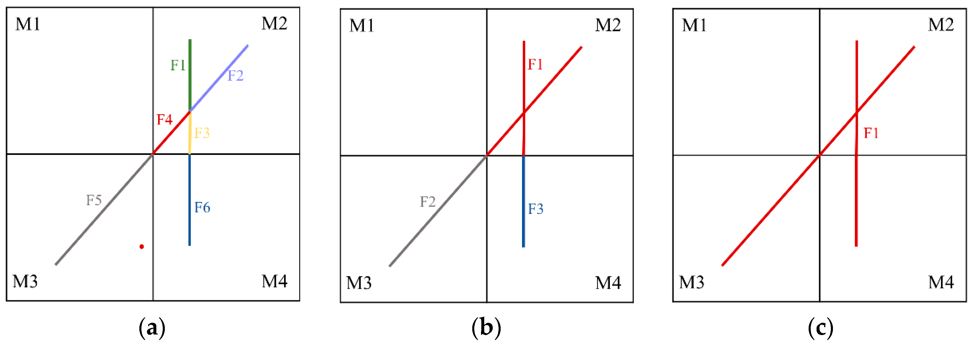
EDFM creates fracture elements connected with corresponding matrix blocks (each represents a matrix element) to account for the mass transfer between matrix and fractures. Once a fracture penetrates a matrix block, an additional element is created to represent the fracture segment in the physical domain (Figure 1a). Each individual fracture is discretized into several fracture elements by the fracture intersections (Figure 1b) and the matrix block boundaries (Figure 1c).
Thus, there exist three kinds of connections: matrix–matrix (M–M), fracture–fracture (F–F), and matrix–fracture (M–F). The transmissibility of each connection can be calculated referring to Equation (7).
The parameters for the M–M connection give clear physical meanings, and so the transmissibility can be easily obtained. For the F–F connection, a simplified approximation from Karimi–Fard [23] is used. The two-point flux approximation scheme is:
where is the absolute permeability of fracture, is the common interface area for these two fracture elements, and and are the average distances from fracture elements 1 and 2 to the common interface.
Transmissibility of M–F depends on the matrix permeability and fracture geometry. When a fracture segment fully penetrates a matrix block, EDFM assumes a uniform pressure gradient in the matrix element, and that pressure gradient is normal to the fracture plane, creating a linear pressure distribution assumption. Then, the M–F transmissibility referring to the equation:
where is the area of the fracture element on one side, is the absolute permeability of matrix (when using the harmonically weighted average permeability, the huge fracture permeability can be ignored), and is the average normal distance from matrix to fracture, which is calculated as:
where is the volume of the matrix element, is the volume element of matrix, and is the distance from the volume element to the fracture plane. If the fracture does not fully penetrate the matrix element, most of the EDFMs make the same assumption as Li [29] that the transmissibility is proportional to the area of the fracture element inside the matrix element, which actually further simplifies the previous linear pressure distribution assumption.
2.3. The Improvement of iEDFM
The integrally embedded discrete fracture model (iEDFM) is implemented on EDFM with a new gridding method, a semi-analytic matrix-fracture transmissibility equation from a more realistic pressure distribution assumption inside the matrix element, which would improve simulation accuracy and expand the scope of application. An iEDFM preprocessor was developed with the inputs of reservoir features and fracture geometries. The gridding and transmissibility calculation processes are conducted in this preprocessor.
In Figure 2, we illustrate the procedure to add fracture elements with a 2D case with 4 matrix blocks and 2 fractures. Figure 2a shows that in EDFM, 6 fracture elements have to be added with 14 F–F connections and 6 F–M connections because of the matrix element boundaries and fracture intersections. However, in iEDFM, the fractures can be embedded integrally—either discretizing by matrix element boundaries (Figure 2b) or taking the intersecting fracture group as one element (Figure 2c) is permitted. As a result, the number of fracture elements can be reduced to 3 or 1, and the number of F–F and F–M connections can be reduced to 2 or 0, 3 or 3.
With the fracture added, we determined the calculation method of transmissibility in iEDFM. For M–M and F–F connections, Equations (7) and (8) are applicable. However, other than using Equation (10), iEDFM has a new semi-analytic transmissibility equation for M–F connections.
When calculating M–F transmissibility in iEDFM, the analytic solution of pressure distribution around the fractures and superposition principle of potential are applied. The detailed method will be explained later.
In general, EDFM has four weaknesses which have been overcome by iEDFM:
- The pressure difference between adjacent fracture pieces is relatively small due to the high conductivity in the fracture. Therefore, such fine gridding for fracture in EDFM may bring unnecessary calculation costs and difficulty in convergence;
- When the matrix block is coarse or the embedded fractures are more complicated, the linear assumption in EDFM is too rough (showed in Case 1);
- If there are more than one fracture pieces inside one matrix element or the fracture has complex geometries, the pressure distribution inside the matrix element will no longer be available, which will limit the application of EDFM (shown in Case 1(c) and Case 3);
- Only the fracture piece and its background matrix block are used for the transmissibility calculation, while the global fracture network is not taken into consideration. For example, when calculating the transmissibility of F5–M3 in Figure 2a, according to the linear pressure distribution assumption in EDFM, the pressure drop at the red point is only influenced by F5. This is inaccurate because there is also F6 nearby, which will also cause a pressure drop at the red point (showed in Case 1(b)).
2.4. Calculation of M–F Transmissibility in iEDFM
The M–F transmissibility calculation is based on the assumption of pressure distribution near the fracture. The linear pressure distribution assumed in EDFM is rough, especially when the embedded fractures are non-penetrating or complicated. In iEDFM, fractures can be considered as a bunch of point sinks. Around each point sink, an analytic pressure distribution formula exists. Then, the superposition principle of potential allows us to obtain the semi-analytic pressure distribution near the fracture. With this pressure distribution, the M–F transmissibility equation is obtained.
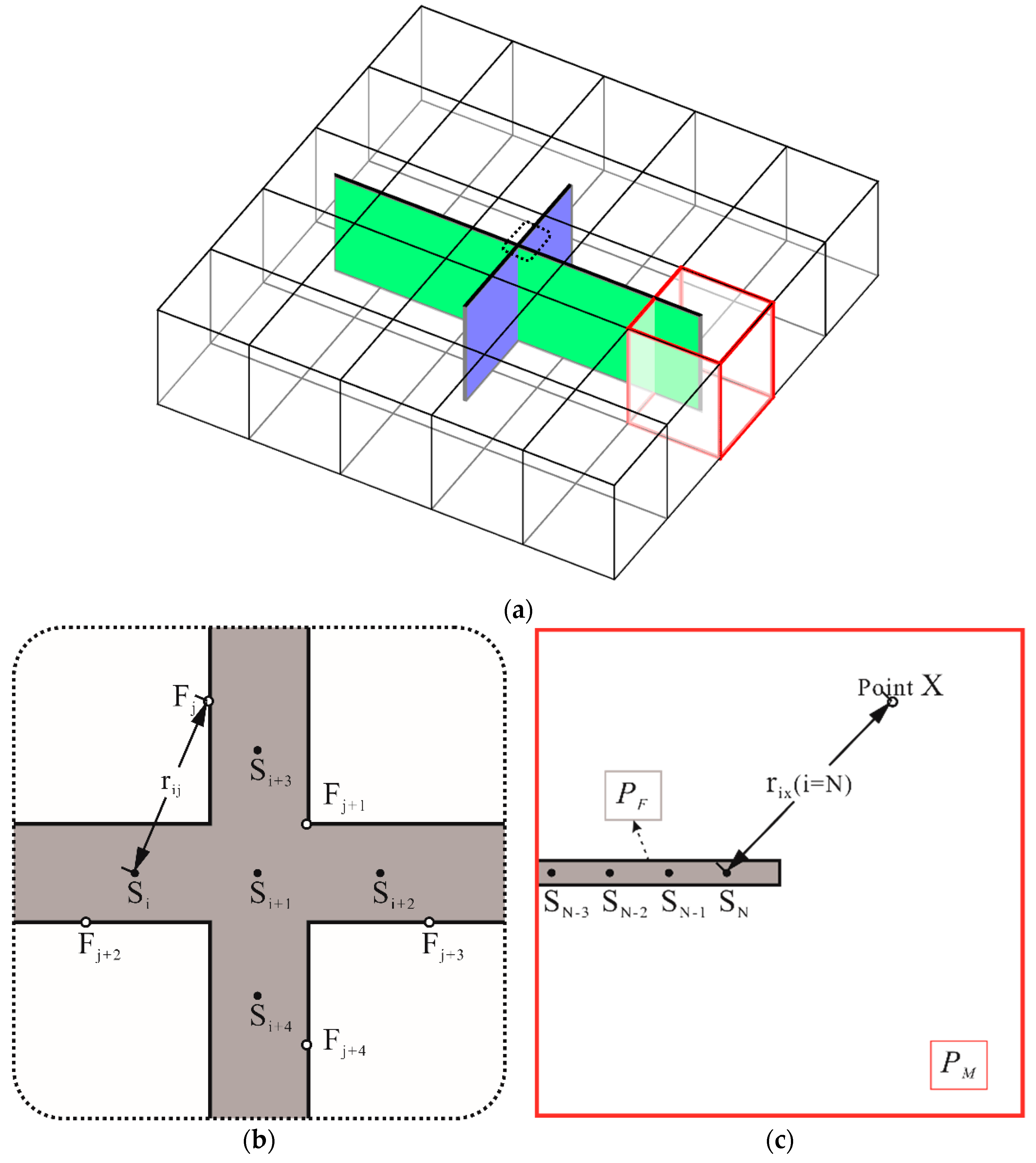
Given a 2D gridded fractured reservoir as an example (Figure 3a), we could take these two intersecting fractures as one element (iEDFM gridding method II) and consider the incompressible steady state single-phase flow in this reservoir.
2.4.1. Point Sinks Imitate the Fracture
The pressure of the fracture element is PF (for the iEDFM gridding method I, a fracture piece in each matrix block has a different pressure, but the formula derivation is also similar, as follows).
We use point sink Si (i = 1 to N) to replace whole intersecting fractures. If the point sinks are dense enough (e.g., more than 50 sinks inside one matrix block), the pressure distribution near the fracture could be imitated near these point sinks. Point Fj (j = 1 to N) is on the surface of the fracture, thus having the same fracture pressure PF. The top view of the dotted frame part in Figure 3a is presented in Figure 3b.
We define a potential:
when the flow reaches the steady state, we have the analytic potential distribution formula of a single point sink from the integral of the plane radial flow equation:
Then, the N-dimensional linear equations are obtained from Equation (13) and the superposition principle of potential:
where is the flow rate of the point sink Si, is the height of the reservoir, is the distance between the point sink Si and the point Fj, and C and c are constant numbers. We define:
where can be solved out from Equation (14).
2.4.2. The Semi-Analytic Calculation Method
Here, we consider the transmissibility between a specific matrix element (for example, the red matrix block in Figure 3a, the top view shown in Figure 3c and the fracture element. The average pressure of the whole matrix element (block) is PM.
Similar to Equation (14), the potential of point X near the fracture inside this specific matrix element can be determined by:
Thus, we obtain:
Combining Equations (16) and (17) and the definition of transmissibility (Equation (4)), the M–F transmissibility and the pressure anywhere inside the matrix block can be calculated by:
where:
where is the volume of the specific matrix element, means that the point is inside this matrix block, is an element volume of this matrix element, is the distance between the point sink Si and . is only related to the properties of the reservoir and can be determined at the step of pre-processing before the simulation starts.
For the 3D situation, referring to Equations (6) and (12), the analytic potential distribution formula of a single point sink is:
After a similar derivation, the—F transmissibility and the pressure distribution can be written as:
where,
3. Verifications and Applications
In the following simulation studies, we present four cases to demonstrate the applicability of iEDFM.
First, a single-phase case is considered to demonstrate the improvement of iEDFM upon EDFM. Then, in the second case, we demonstrate the accuracy of our model by comparing the flow rates and saturation profiles with the fine-grid model through a flooding test. Both gridding methods I and II are used in this case. Then, a nonplanar fractures case is presented to show the applicability of iEDFM for a complex geometry situation. At last, a 3D field case demonstrates the potential application of iEDFM in real field studies.
Most of the reservoir properties and operation parameters were kept the same in all the cases, as shown in Table 1.
3.1. Case 1: Constant Pressure Pumping from Fractures
The calculation method of M–F transmissibility is based on the assumption of pressure distribution pattern in the vicinity of fractures. EDFM assumes a uniform pressure gradient in the matrix element, while iEDFM uses a semi-analytic method to calculate the pressure distribution.
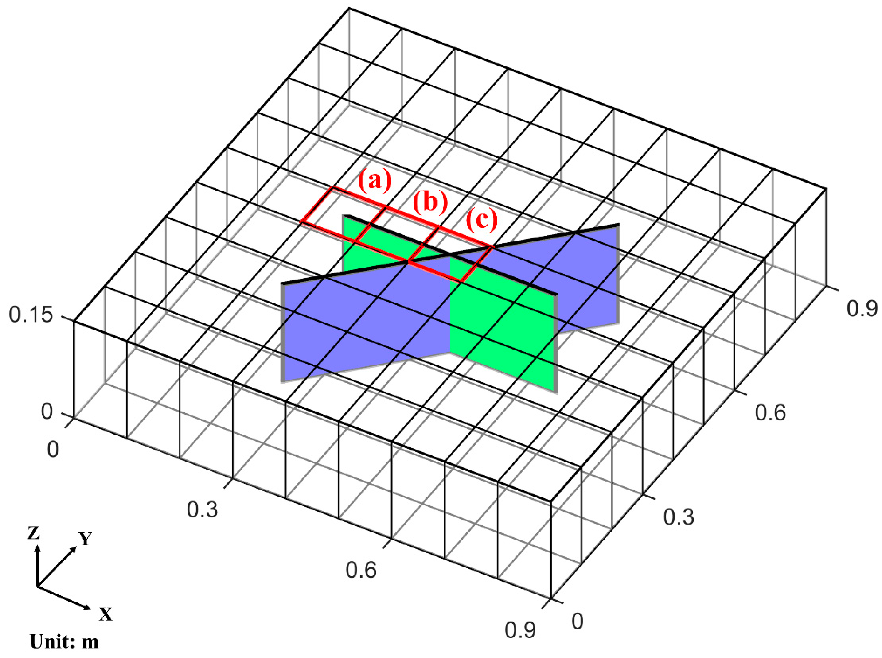
In this case, we consider an ideal reservoir with two intersecting fractures (Figure 4), using simulation results from the fine-grid model to verify the effectiveness of iEDFM over EDFM. EDFM or iEDFM simulation is not conducted in this case. Only the pressure distribution and M–F transmissibility for red block (a)/(b)/(c) are calculated through the pre-processing procedure of iEDFM and EDFM, comparing with the simulation result of the whole reservoir of the fine-grid model.
Single-phase fluid (water) is pumping out from the constant pressure vertical fractures simulated in the fine-grid model discretized by 900 × 900 fine gridblocks horizontally. The element dimensions are non-uniform in the x and y directions to accommodate refinement around fractures. The widths of the fracture elements and their adjacent matrix elements were equal to the fracture aperture. Table 2 supplements some parameters in addition to Table 1.
This pumping pressure represents the pressure of the fracture element, and the average pressure of the matrix inside the red blocks represents the pressure of the matrix element. The fluid exchange can be obtained from simulation results of the fine-grid model. Therefore, the equivalent M–F transmissibility by the fine-grid model can be calculated through Equation (4).
Figure 5b shows that the transmissibility calculation methods in EDFM and iEDFM are more accurate when the fracture fully penetrates the matrix block. It can be seen from Figure 5a that when the fracture does not fully penetrate, the EDFM method will cause some error which cannot be ignored, which is in agreement with the estimation by Xu [30], while the iEDFM method can still be relatively accurate in this situation. In Figure 5c, we can see that the EDFM method produces more obvious errors in the complex situation with fracture intersection, whereas the iEDFM method is still relatively accurate.
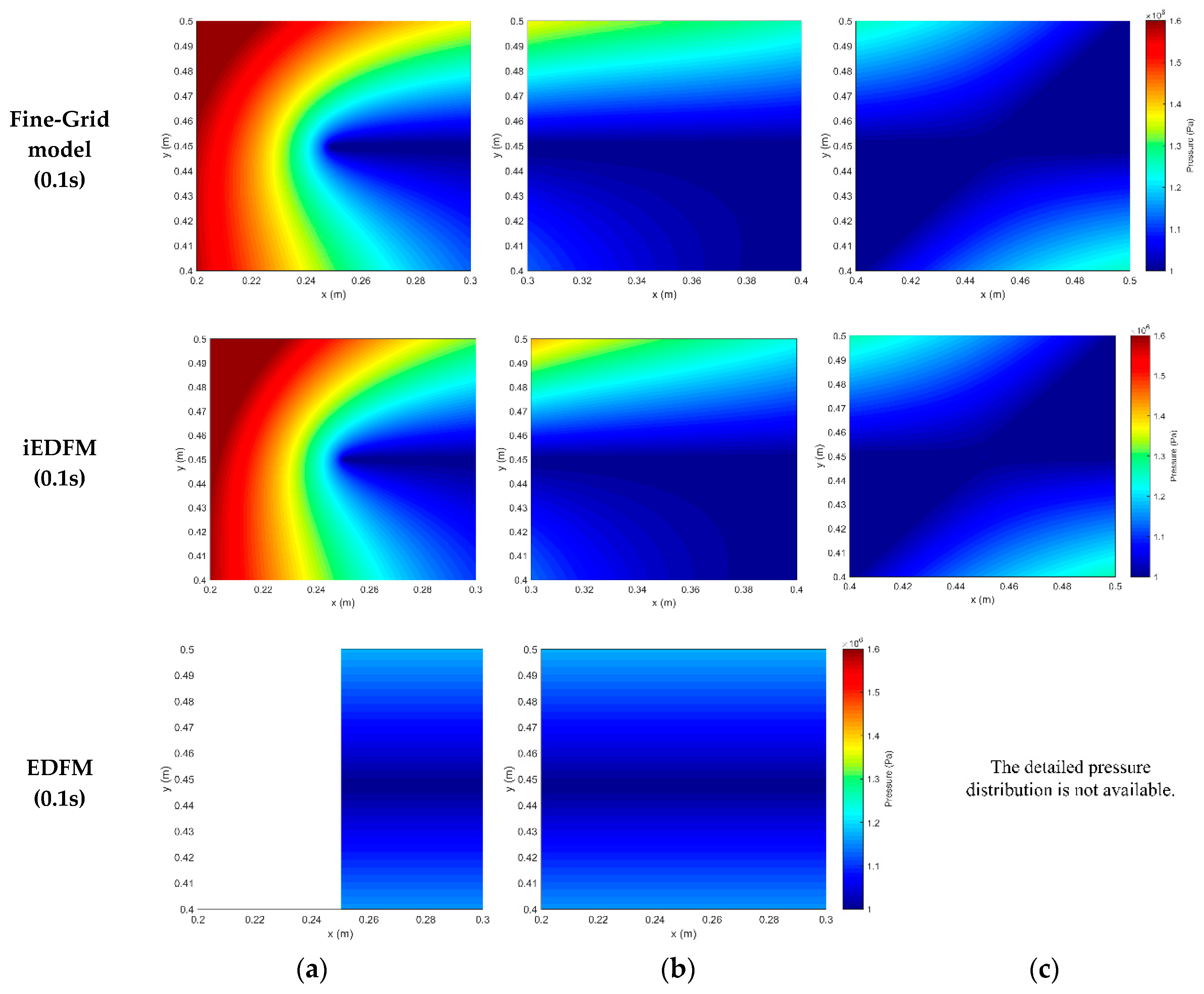
The errors and differences are mainly due to different assumptions regarding the pressure distribution in the vicinity of fractures. In Figure 6, the pressure profiles in block (a) (b) and (c) after 0.1s of pumping are presented. Three kinds of pressure profiles are considered here: pressure distribution calculated by the fine-grid method, and the pressure distribution assumed by EDFM / iEDFM.
As shown in Figure 6, the results of the fine-grid model are quite similar to iEDFM, with negligible difference. However, the results of EDFM indicate that when the matrix block is not fully penetrated by the fracture (Figure 6a) or the embedded fractures are complicated (Figure 6c), the linear distribution of EDFM’s assumption can be rough. Even if the fracture penetrates the block (b), the linear distribution still does not exactly reflect the real situation, because of the effect of the fracture segment outside this matrix block, which EDFM does not take into consideration but iEDFM does.
In summary, iEDFM has a more accurate M–F transmissibility calculation method based on a more realistic pressure distribution assumption. In addition, iEDFM can assume a specific pressure field for any complex embedding situation. If pressure-related physical properties, such as adsorption analysis and diffusion effects, need to be considered, iEDFM is able to show a greater applicability.
3.2. Case 2: Intersecting-Fractured Reservoir Flooding Test
Figure 7 shows a 2D fractured reservoir containing three intersecting vertical fractures. This case is a displacement of oil by water, applied in the fine-grid model and the iEDFM model. Table 3 supplements some parameters of this case in addition to Table 1, which will also be used in the following cases.
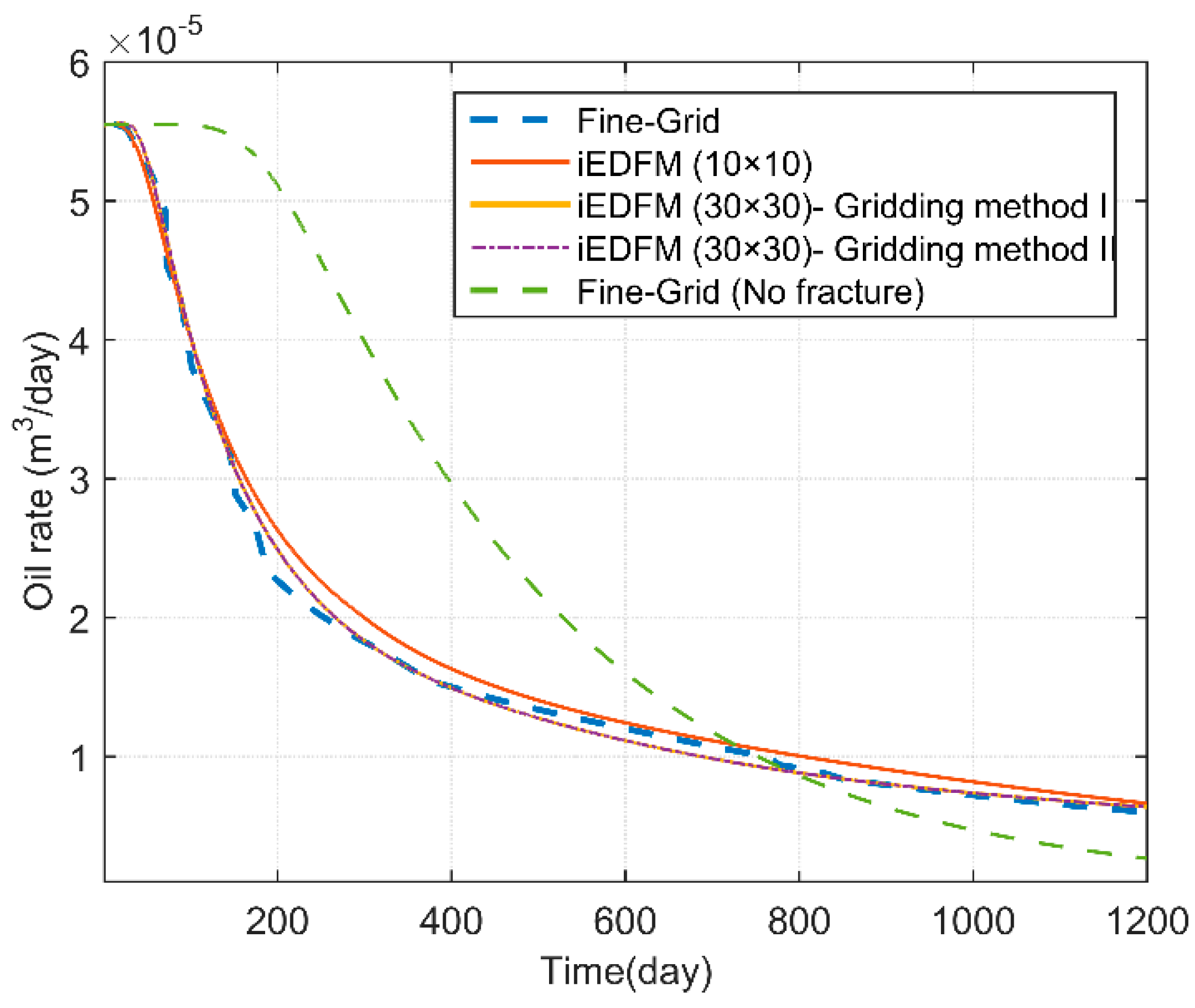
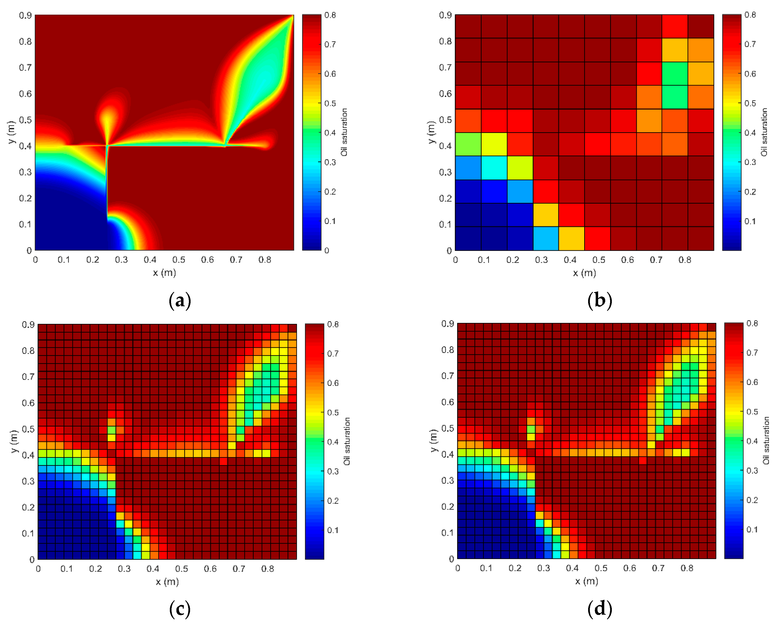
For the fine-grid simulation, the grid is 900 × 900 elements in the x and y directions. For the iEDFM simulation, two sets of uniform matrix grids (30 × 30/10 × 10) are used. Gridding methods I and II are also compared in this case (gridding method I is applied if not mentioned, as below). The oil rate and the profiles of oil saturation after 115 days of water injection (8.64 × 10⁻⁵ m3/day) calculated by iEDFM and fine-grid model are presented in Figure 8 and Figure 9.
Figure 8 compares the oil production rates, confirming the accuracy of the iEDFM approach. A good agreement exists in both 30 × 30/10 × 10. The curves of gridding methods I and II almost coincide, indicating that the results of these two methods are not much different when the permeability of fracture is much higher than that of the matrix, respectively. A curve of the same reservoir without any fracture is also present on this figure to show the influence of the existence of fractures. The effect of phase behavior on oil saturations is also pronounced in this case, as Figure 9 shows.
The computational times for iEDFM (30 × 30), iEDFM (10 × 10) and the fine-grid model are 9.1 s, 4.3 s and 6.7 h, respectively, which indicates a high efficiency of iEDFM.
3.3. Case 3: Nonplanar-Fractured Reservoir Flooding Test
Recent advances in fracture-diagnostic tools and fracture-propagation models make it necessary to model fractures with complex geometries in reservoir-simulation studies. A nonplanar shape is one of the most common complex geometries [30].
Fractures tend to grow in the direction perpendicular to the minimum horizontal stress. In some cases, the preferred direction of fracture may not keep the same, which often leads to a nonplanar shape.
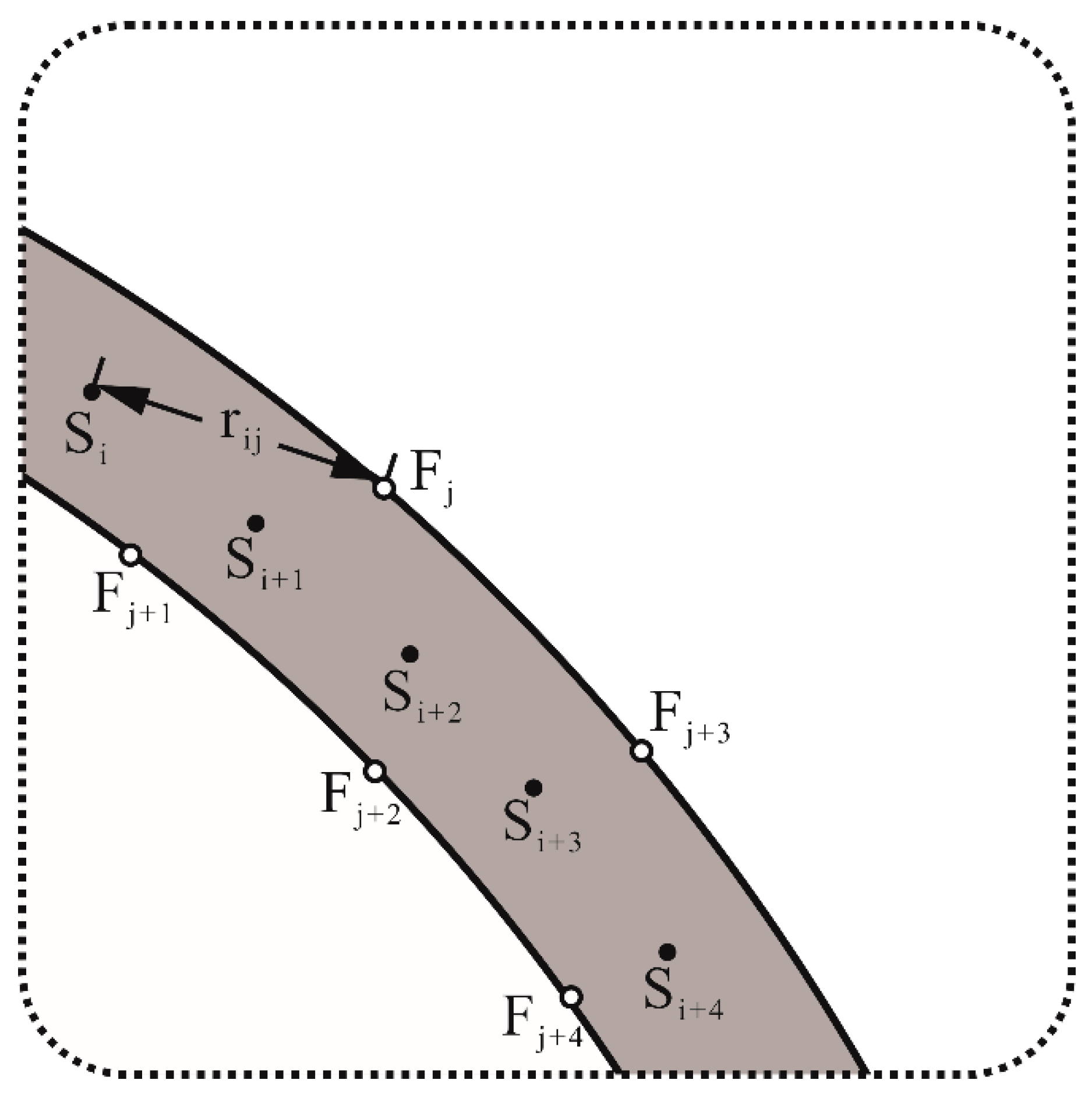
The methodology introduced in this study can be directly applied in a nonplanar fractures case. As Figure 10 shows, the location of the assumed points Si and Fi will reflect the geometry of the fracture. As a result, the semi-analytic method can bring iEDFM enough flexibility in modeling nonplanar fractures.
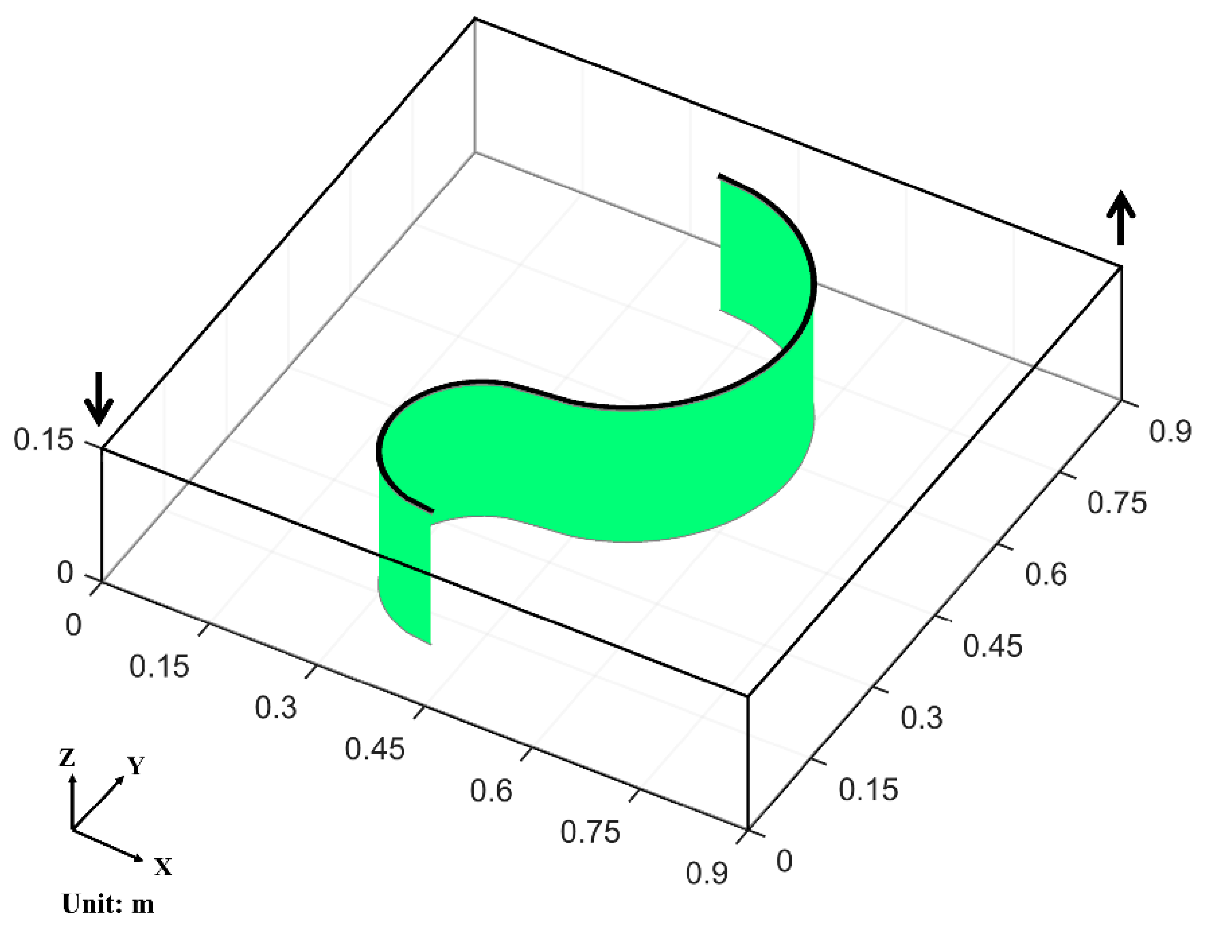
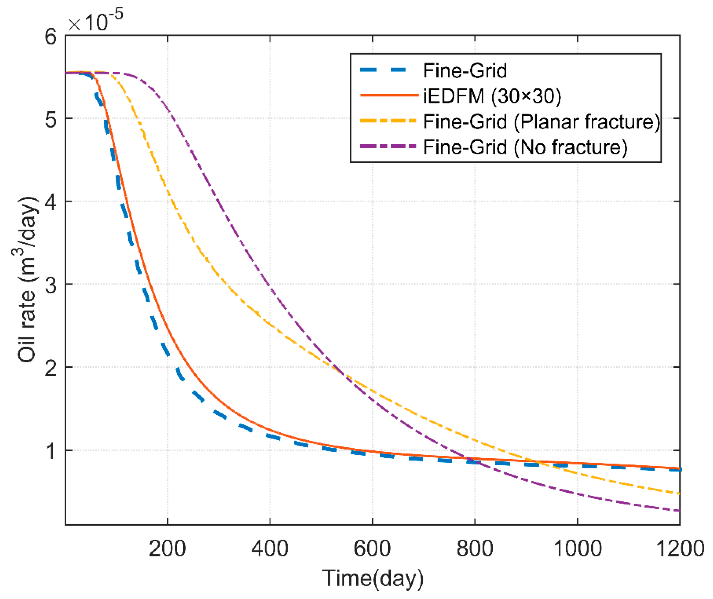
We present an ideal case as shown in Figure 11 in which the fracture is formed as two connected arcs seen in the top view and is vertical in the z direction. The same parameters as Case 2 are applied here, and a fine-grid model similar to Case 2 is built. For the iEDFM simulation, gridding method I and a uniform matrix grid (30 × 30 with one layer in z direction) are used.
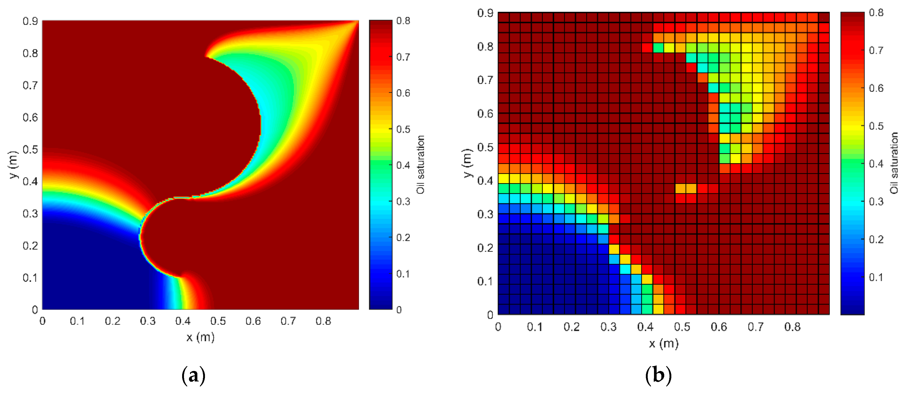
The oil rate curves are presented in Figure 12 and the oil saturation profiles after 115 days of injection are shown in Figure 13, where a good agreement demonstrates the accuracy of the iEDFM in modeling the nonplanar fractures reservoir. The curves of the same reservoir without any fracture and with a planar fracture with the same starting and ending location are also present on this figure to show the influence of the existence of nonplanar fractures.
Actually, as Figure 3b and Figure 10 show, different locations of point Si and Fi are able to reflect any geometry of the fractures, such as fractures with variable apertures and vuggy-fractures, which means that iEDFM is naturally suitable for any other complex geometry cases beside nonplanar fractures.
3.4. Case 4: 3D Case with a Modified Dataset of a Real Field
As mentioned previously, iEDFM can be used as a general procedure in both 2D and 3D cases. In real field applications, the reservoir may have multiple layers, and the height of the fractures can be smaller than the reservoir height. Therefore, a 3D simulation example is presented to show the application of iEDFM in a typical field study.
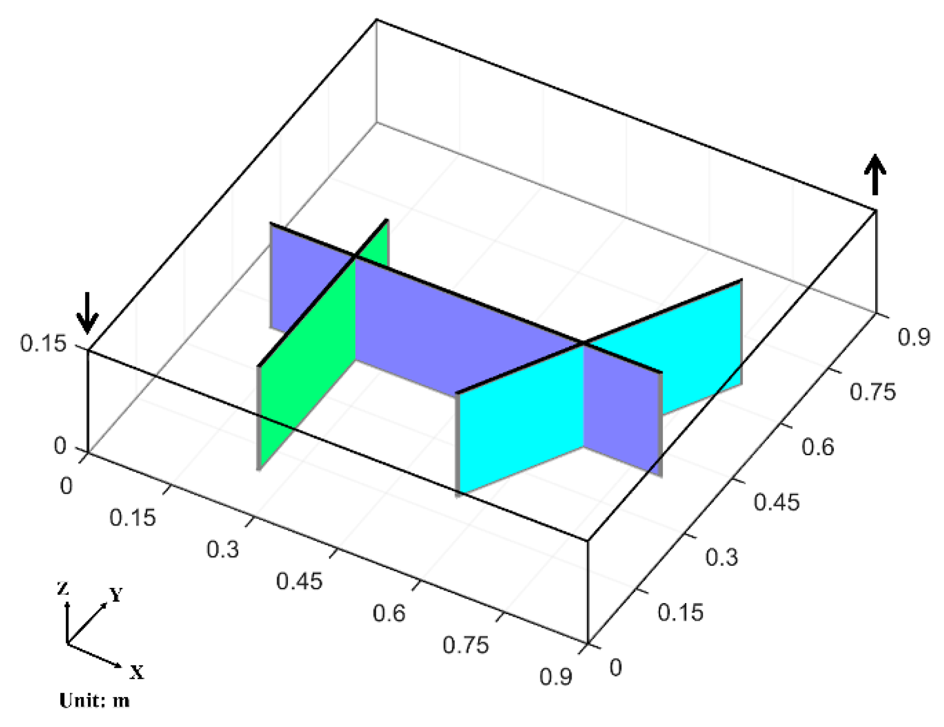
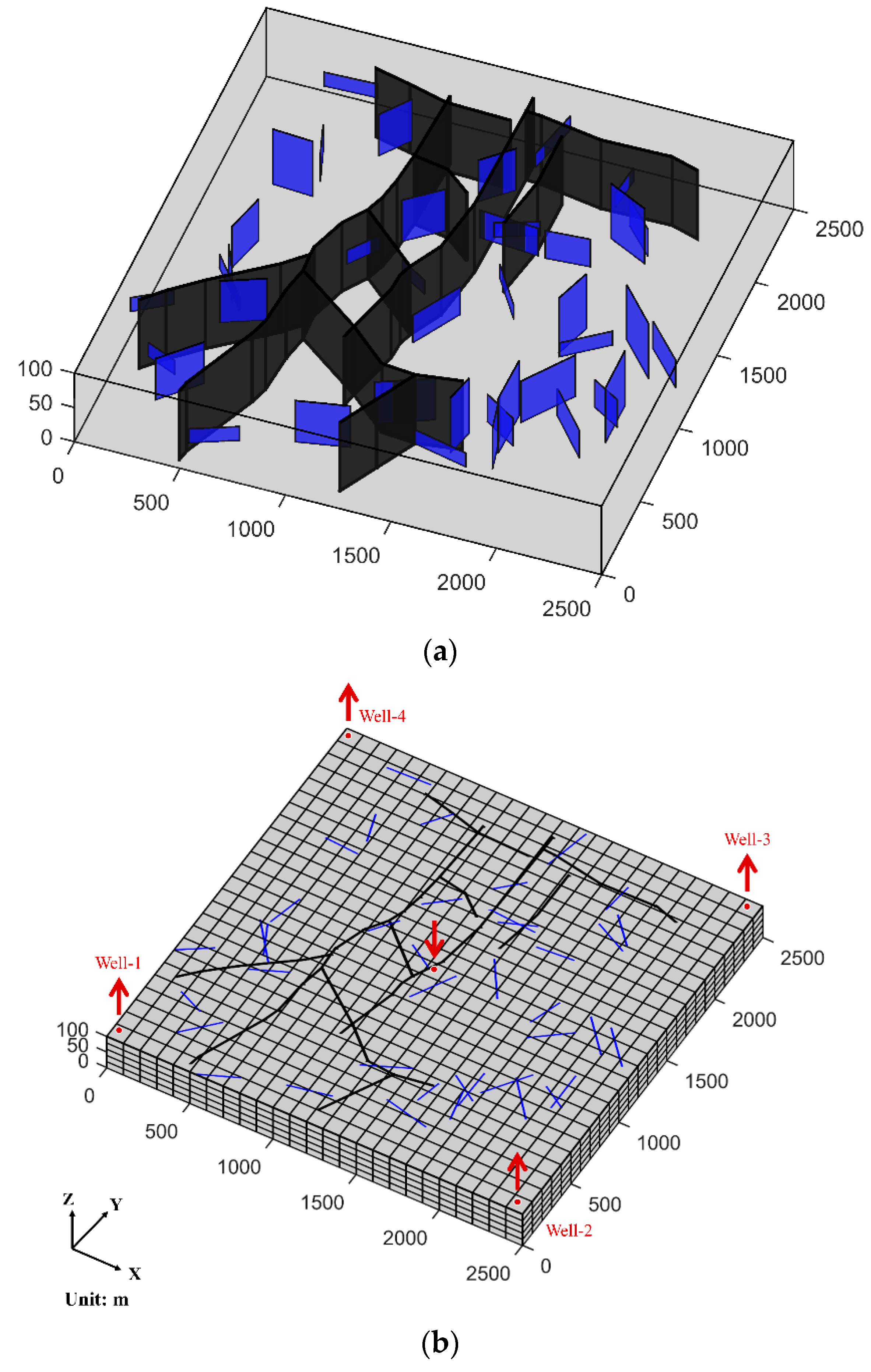
In this case, the geological model is modified from a reported dataset which is interpreted from a 3D seismic survey [35,36]. Some irregular, sparsely distributed large-scale fractures are present as main fractures (black planes in Figure 14a). Some stochastic medium-scale fractures (blue planes in Figure 14a) are added to test iEDFM’s applicability in a complex fracture-network situation. The main fractures and the wells are assumed to extend throughout the entire depth of the reservoir, while the stochastic medium-scale fractures are of different heights. Figure 14b shows the matrix grids (25 × 25 × 5) and the position of fractures and wells. An injection well (4 × 10⁴ m3/day) is placed in the center, while producers are placed in four corners of the reservoir. Again, the reservoir without any fracture is also simulated as a comparison.
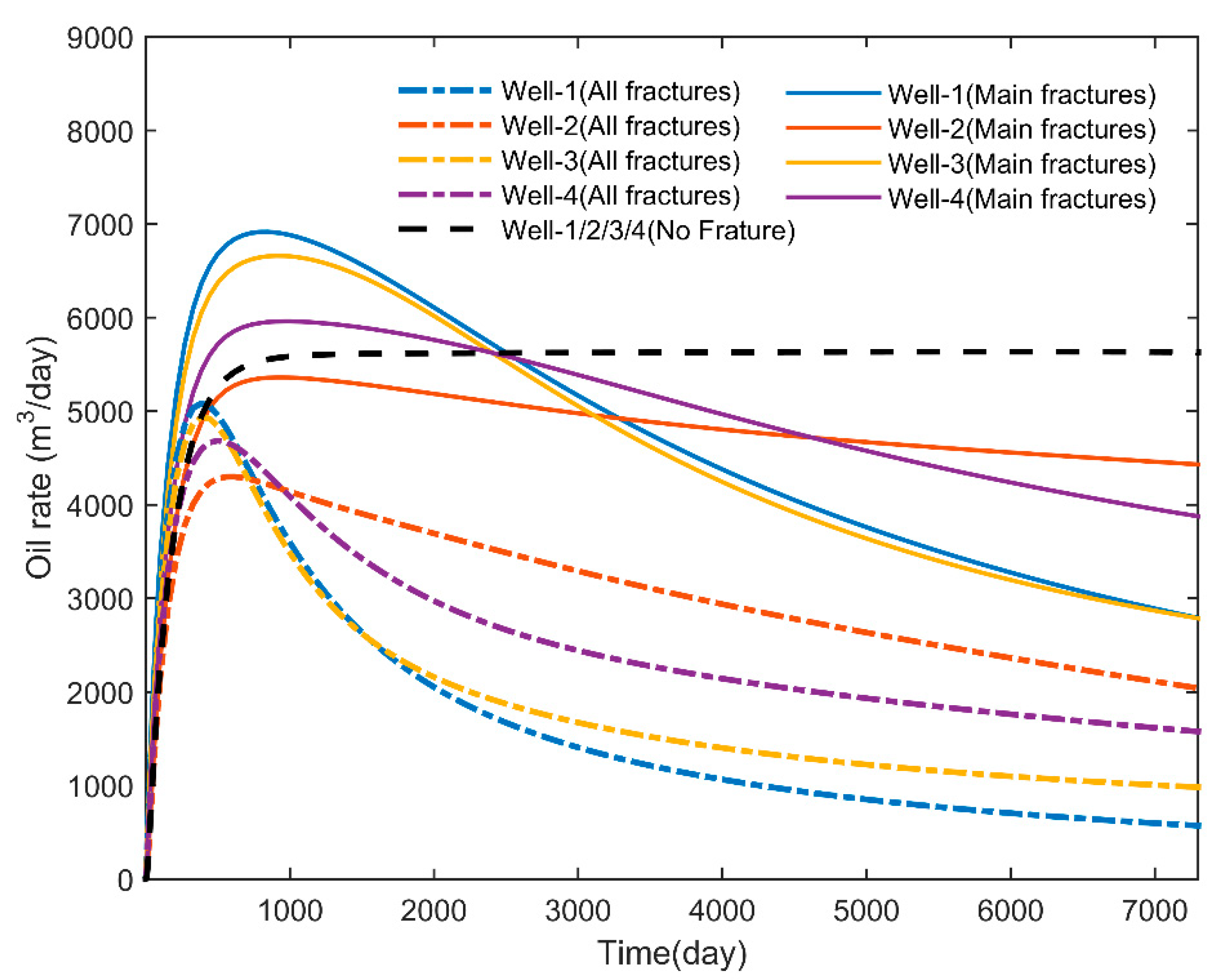
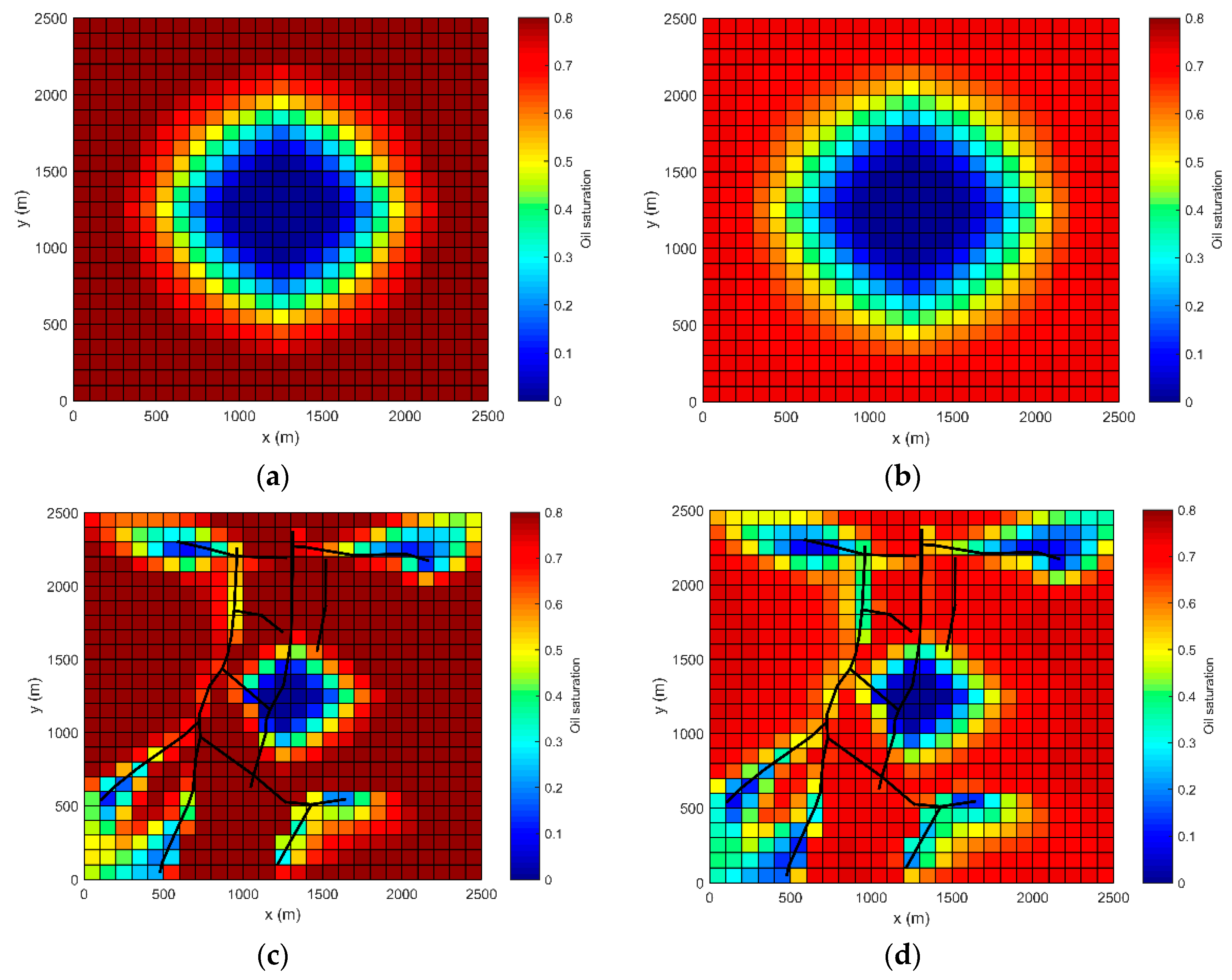
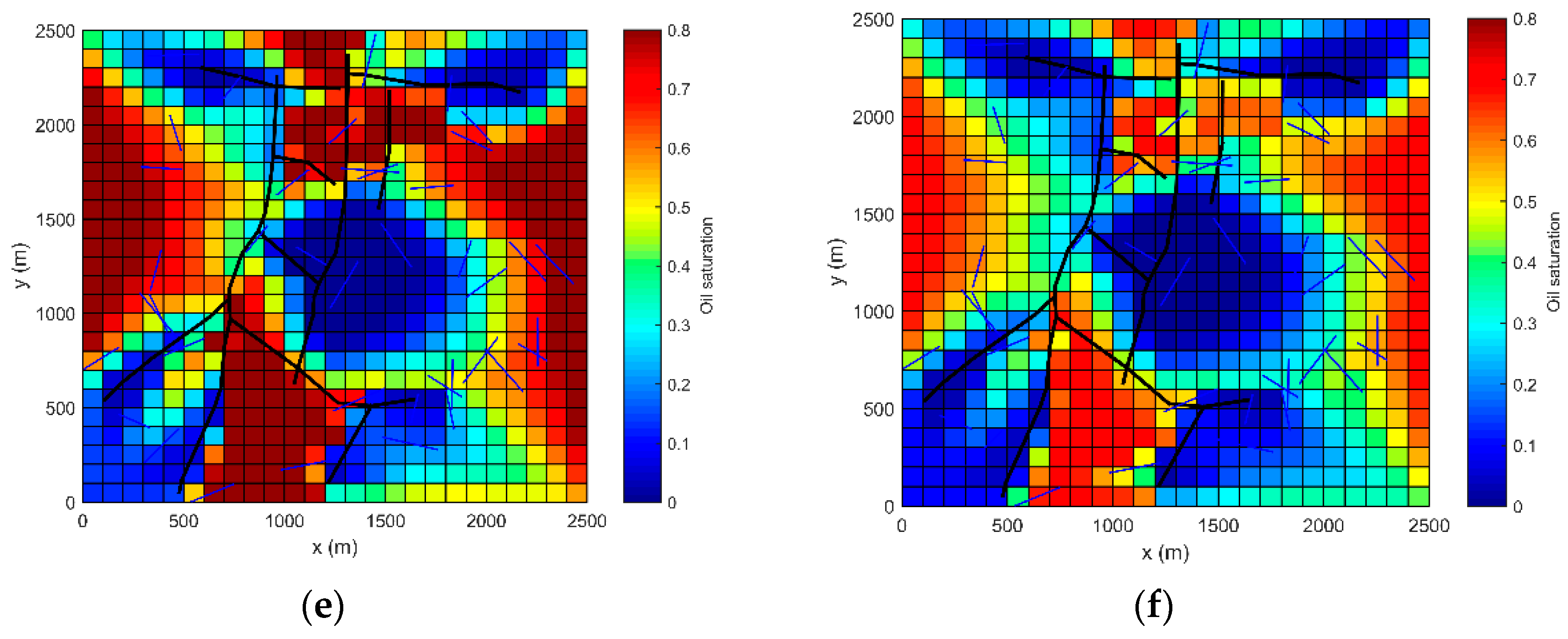
The oil rate curves are presented in Figure 15. The curves of wells 1–4 in the reservoir without fractures are coincident because of the symmetry. The pressure profiles of the top and bottom layers after 7300 days of injection are shown in Figure 16. As we can see, the reservoir shows strong heterogeneity due to the existence of fractures, and the water’s breakthrough is advanced, which reduces the recovery efficiency. As medium-scale fractures are added, these phenomena become more pronounced. Because of gravity, the average oil saturation of the first layer is higher than that of the bottom layer (0.6952 of Figure 16c than 0.5671 of Figure 16d, respectively).
The case study showed the applicability of the iEDFM in reservoirs with complex fracture networks. The influence of different scales of fractures can be modeled appropriately by iEDFM. The 3D multiphase simulation example demonstrates the potential application of the iEDFM in real field studies.
4. Conclusions and Future Work
In this study, we developed a new approach called the integrally embedded discrete fracture model (iEDFM). This approach, for the first time, avoids the limitations of the need to subdivide fracture elements in EDFM.
In iEDFM, we can arbitrarily grid fractures according to the requirements, and then embed them integrally in matrix blocks. As a precise pressure distribution assumption inside the matrix blocks is introduced, we can obtain a semi-analytic calculation method of matrix-fracture transmissibility. As a result, the simulation accuracy is improved and the application is also expanded to fractures with complex geometries. Several cases have been presented to support these conclusions. The potential application of the iEDFM in real field studies has also been testified through a 3D case.
Applying the iEDFM to real field study and guiding production is our ultimate goal. Thus, heterogeneous and more complex actual reservoir examples with actual production data will be considered in our on-going project.
Author Contributions
R.S. and Y.D. conceived of the idea. R.S. developed the theory and conducted the computations. Y.D. guided the data analysis and supervised the work. This paper was written by R.S. and modified by Y.D.
Funding
This research received no external funding.
Acknowledgments
This work was supported by National Science and Technology Major Project of China (2016ZX05014) and National Natural Science Foundation of China (51674010).
Conflicts of Interest
The authors declare no conflict of interest.
References
- Saller, S.P.; Ronayne, M.J.; Long, A.J. Comparison of a Karst Groundwater Model with and without Discrete Conduit Flow. Hydrogeol. J. 2013, 21, 1555–1566. [Google Scholar] [CrossRef]
- Gurpinar, O.M.; Kossack, C.A. Realistic Numerical Models for Fractured Reservoirs. SPE J. 2000, 5, 485–491. [Google Scholar] [CrossRef]
- Basquet, R.; Cohen, C.E.; Bourbiaux, B. Fracture Flow Property Identification: An Optimized Implementation of Discrete Fracture Network Models. In Proceedings of the SPE Middle East Oil and Gas Show and Conference, Manama, Kingdom of Bahrain, 12–15 March 2005. [Google Scholar]
- Sarda, S.; Jeannin, L.; Basquet, R.; Bourbiaux, B. Hydraulic Characterization of Fractured Reservoirs: Simulation on Discrete Fracture Models. In Proceedings of the SPE Reservoir Simulation Symposium, Houston, TX, USA, 11–14 February 2001. [Google Scholar]
- Yan, B.; Mi, L.; Chai, Z.; Wang, Y.; Killough, J.E. An Enhanced Discrete Fracture Network Model for Multiphase Flow in Fractured Reservoirs. J. Pet. Sci. Eng. 2018, 161, 667–682. [Google Scholar] [CrossRef]
- Warren, J.E.; Root, P.J. The Behavior of Naturally Fractured Reservoirs. SPE J. 1963, 3, 245–255. [Google Scholar] [CrossRef]
- Kazemi, H. Pressure Transient Analysis of Naturally Fractured Reservoirs with Uniform Fracture Distribution. SPE J. 1969, 9, 451–462. [Google Scholar] [CrossRef]
- Swaan, A.D. Theory of Waterflooding in Fractured Reservoirs. SPE J. 1978, 18, 117–122. [Google Scholar] [CrossRef]
- Gilman, J.R. Efficient Finite-Difference Method for Simulating Phase Segregation in the Matrix Blocks in Double-Porosity Reservoirs. SPE Reserv. Eng. 1986, 1, 403–413. [Google Scholar] [CrossRef]
- Gilman, J.R.; Kazemi, H. Improved Calculations for Viscous and Gravity Displacement in Matrix Blocks in Dual-Porosity Simulators. J. Pet. Technol. 1988, 40, 60–70. [Google Scholar] [CrossRef]
- Pruess, K.; Narasimhan, T.N. Practical Method for Modeling Fluid and Heat Flow in Fractured Porous Media. SPE J. 1985, 25, 14–26. [Google Scholar] [CrossRef]
- Wu, Y.S.; Pruess, K. Multiple-porosity Method for Simulation of Naturally Fractured Petroleum Reservoirs. SPE Reserv. Eng. 1988, 3, 335–350. [Google Scholar] [CrossRef]
- Fung, L.S.K. Simulation of Block-to-Block Processes in Naturally Fractured Reservoirs. SPE Reserv. Eng. 1991, 6, 477–484. [Google Scholar] [CrossRef]
- Wu, Y.; Di, Y.; Kang, Z.; Fakcharoenphol, P. A Multiple-Continuum Model for Simulating Single-phase and Multiphase Flow in Naturally Fractured Vuggy Reservoirs. J. Pet. Sci. Eng. 2011, 78, 13–22. [Google Scholar] [CrossRef]
- Sun, H.; Chawathe, A.; Hoteit, H.; Shi, X.; Li, L. Understanding Shale Gas Flow Behavior Using Numerical Simulation. SPE J. 2015, 20, 142–154. [Google Scholar] [CrossRef]
- Yan, B.; Alfi, M.; An, C.; Cao, Y.; Wang, Y.; Killough, J.E. General Multi-porosity Simulation for Fractured Reservoir Modeling. J. Nat. Gas Sci. Eng. 2016, 33, 777–791. [Google Scholar] [CrossRef]
- Noorishad, J.; Mehran, M. An Upstream Finite-Element Method for Solution of Transient Transport-Equation in Fractured Porous-Media. Water Resour. Res. 1982, 18, 588–596. [Google Scholar] [CrossRef]
- Karimi-Fard, M.; Firoozabadi, A. Numerical Simulation of Water Injection in Fractured Media Using the Discrete-Fracture Model and the Galerkin Method. SPE Reserv. Eval. Eng. 2003, 6, 117–126. [Google Scholar] [CrossRef]
- Monteagudo, J.; Firoozabadi, A. Control-Volume Method for Numerical Simulation of Two-phase Immiscible Flow in Two- and Three-Dimensional Discrete-Fractured Media. Water Resour. Res. 2004, 40. [Google Scholar] [CrossRef]
- Hoteit, H.; Firoozabadi, A. Compositional Modeling of Discrete-Fractured Media without Transfer Functions by the Discontinuous Galerkin and Mixed Methods. SPE J. 2006, 11, 341–352. [Google Scholar] [CrossRef]
- Matthai, S.K.; Mezentsev, A.; Belayneh, M. Finite Element-Node-Centered Finite-Volume Two-Phase-Flow Experiments with Fractured Rock Represented by Unstructured Hybrid-Element Meshes. SPE Reserv. Eval. Eng. 2007, 10, 740–756. [Google Scholar] [CrossRef]
- Sandve, T.H.; Berre, I.; Nordbotten, J.M. An Efficient Multi-Point Flux Approximation Method for Discrete Fracture-Matrix Simulations. J. Comput. Phys. 2012, 231, 3784–3800. [Google Scholar] [CrossRef]
- Karimi-Fard, M.; Durlofsky, L.J.; Aziz, K. An Efficient Discrete-Fracture Model Applicable for General-Purpose Reservoir Simulators. SPE J. 2004, 9, 227–236. [Google Scholar] [CrossRef]
- Olorode, O.M.; Freeman, C.M.; Moridis, G.J.; Blasingame, T.A. High-Resolution Numerical Modeling of Complex and Irregular Fracture Patterns in Shale-Gas Reservoirs and Tight Gas Reservoirs. SPE Reserv. Eval. Eng. 2013, 16, 443–455. [Google Scholar] [CrossRef]
- Al-Hinai, O.; Signh, G.; Pencheva, G.; Almani, T.; Wheeler, M.F. Modeling Multiphase Flow with Nonplanar Fractures. In Proceedings of the SPE Reservoir Simulation Symposium, The Woodlands, TX, USA, 18–20 February 2013. [Google Scholar]
- Moinfar, A.; Varavei, A.; Sepehrnoori, K.; Johns, R.T. Development of an Efficient Embedded Discrete Fracture Model for 3d Compositional Reservoir Simulation in Fractured Reservoirs. SPE J. 2014, 19, 289–303. [Google Scholar] [CrossRef]
- Boyle, E.J.; Sams, W.N. Nfflow: A Reservoir Simulator Incorporating Explicit Fractures. In Proceedings of the SPE Western Regional Meeting, Bakersfield, CA, USA, 21–23 March 2012. [Google Scholar]
- Lee, S.H.; Lough, M.F.; Jensen, C.L. Hierarchical Modeling of Flow in Naturally Fractured Formations with Multiple Length Scales. Water Resour. Res. 2001, 37, 443–455. [Google Scholar] [CrossRef]
- Li, L.; Lee, S.H. Efficient Field-Scale Simulation of Black Oil in a Naturally Fractured Reservoir Through Discrete Fracture Networks and Homogenized Media. SPE Reserv. Eval. Eng. 2008, 11, 750–758. [Google Scholar] [CrossRef]
- Xu, Y.; Cavalcante Filho, J.S.A.; Yu, W.; Sepehrnoori, K. Discrete-Fracture Modeling of Complex Hydraulic-Fracture Geometries in Reservoir Simulators. SPE Reserv. Eval. Eng. 2017, 20, 403–422. [Google Scholar] [CrossRef]
- Yu, W.; Xu, Y.; Liu, M.; Wu, K.; Sepehrnoori, K. Simulation of Shale Gas Transport and Production with Complex Fractures Using Embedded Discrete Fracture Model. AIChE J. 2018, 64, 2251–2264. [Google Scholar] [CrossRef]
- Li, W.; Dong, Z.; Lei, G. Integrating Embedded Discrete Fracture and Dual-Porosity, Dual-Permeability Methods to Simulate Fluid Flow in Shale Oil Reservoirs. Energies 2017, 10. [Google Scholar] [CrossRef]
- Tene, M.; Bosma, S.B.M.; Al Kobaisi, M.S.; Hajibeygi, H. Projection-Based Embedded Discrete Fracture Model (pEDFM). Adv. Water Resour. 2017, 105, 205–216. [Google Scholar] [CrossRef]
- Wu, Y.S. A Virtual Node Method for Handling Well Bore Boundary Conditions in Modeling Multiphase Flow in Porous and Fractured Media. Water Resour. Res. 2000, 36, 807–814. [Google Scholar] [CrossRef]
- Shuck, E.L.; Davis, T.L.; Benson, R.D. Multicomponent 3-D Characterization of a Coalbed Methane Reservoir. Geophysics 1996, 61, 315–330. [Google Scholar] [CrossRef]
- Zhang, Y.; Gong, B.; Li, J.; Li, H. Discrete Fracture Modeling of 3D Heterogeneous Enhanced Coalbed Methane Recovery with Prismatic Meshing. Energies 2015, 8, 6153–6176. [Google Scholar] [CrossRef] [Green Version]
Figure 1.
Explanation of the embedded discrete fracture model (EDFM) gridding [26]: (a) a fracture segment is embedded in a matrix block; (b) two fracture planes intersect in a matrix block; and (c) two fracture segments embedded in neighboring matrix blocks.
Figure 1.
Explanation of the embedded discrete fracture model (EDFM) gridding [26]: (a) a fracture segment is embedded in a matrix block; (b) two fracture planes intersect in a matrix block; and (c) two fracture segments embedded in neighboring matrix blocks.

Figure 2.
Explanation of the integrally embedded discrete fracture model (iEDFM) gridding: (a) EDFM gridding method; (b) iEDFM gridding method I—discretizing by matrix element boundaries; and (c) iEDFM gridding method II—taking the intersecting fracture group as one element.
Figure 2.
Explanation of the integrally embedded discrete fracture model (iEDFM) gridding: (a) EDFM gridding method; (b) iEDFM gridding method I—discretizing by matrix element boundaries; and (c) iEDFM gridding method II—taking the intersecting fracture group as one element.

Figure 3.
Illustration showing the calculation of M–F transmissibility in iEDFM: (a) a 2D example of the fractured reservoir; (b) the top view of the dotted frame part; and (c) the top view of the red matrix block.
Figure 3.
Illustration showing the calculation of M–F transmissibility in iEDFM: (a) a 2D example of the fractured reservoir; (b) the top view of the dotted frame part; and (c) the top view of the red matrix block.

Figure 4.
The fractured reservoir in Case 1. The 9 × 9 grids showed a possible gridding choice for iEDFM or EDFM.
Figure 4.
The fractured reservoir in Case 1. The 9 × 9 grids showed a possible gridding choice for iEDFM or EDFM.

Figure 5.
TM-F of the fine-grid model (equivalent)/iEDFM/EDFM for block (a)/(b)/(c). The equivalent transmissibility calculated by the fine-grid model will change over time until the flow approaches a steady state, while the ones calculated through the pre-processing procedure of iEDFM/EDFM stay the same.

Figure 6.
Pressure distribution profiles after 0.1 s pumping of the fine-grid model/iEDFM (assumed)/EDFM (assumed) for block (a)/(b)/(c).
Figure 6.
Pressure distribution profiles after 0.1 s pumping of the fine-grid model/iEDFM (assumed)/EDFM (assumed) for block (a)/(b)/(c).

Figure 7.
The fractured reservoir in Case 2. A water injector is placed in one corner of the reservoir and a producer is located in the opposite corner.
Figure 7.
The fractured reservoir in Case 2. A water injector is placed in one corner of the reservoir and a producer is located in the opposite corner.

Figure 8.
Comparison of oil production rate by the iEDFM/fine-grid model in Case 2.

Figure 9.
Profiles of oil saturation after 115 days’ injection for Case 2 in: (a) the fine-grid model; (b) iEDFM (10 × 10, gridding method I); (c) iEDFM (30 × 30, gridding method I); and (d) iEDFM (30 × 30, gridding method II).
Figure 9.
Profiles of oil saturation after 115 days’ injection for Case 2 in: (a) the fine-grid model; (b) iEDFM (10 × 10, gridding method I); (c) iEDFM (30 × 30, gridding method I); and (d) iEDFM (30 × 30, gridding method II).

Figure 10.
Schematic of equivalent point sinks and other parameters used in the nonplanar fracture case corresponding to Figure 3b.
Figure 10.
Schematic of equivalent point sinks and other parameters used in the nonplanar fracture case corresponding to Figure 3b.

Figure 11.
The nonplanar-fractured reservoir in Case 3. A water injector (8.64 × 10⁻⁵ m3/day) is located in one corner of the reservoir, and a producer is placed in the opposite corner.
Figure 11.
The nonplanar-fractured reservoir in Case 3. A water injector (8.64 × 10⁻⁵ m3/day) is located in one corner of the reservoir, and a producer is placed in the opposite corner.

Figure 12.
Comparison of oil production rate by the iEDFM/fine-grid model in Case 3.

Figure 13.
Profiles of oil saturation after 115 days’ injection for Case 3 in (a) the fine-grid model and (b) iEDFM (30 × 30).
Figure 13.
Profiles of oil saturation after 115 days’ injection for Case 3 in (a) the fine-grid model and (b) iEDFM (30 × 30).

Figure 14.
(a) Three-dimensional view of main fractures and medium-scale fractures; (b) The matrix grids of the reservoir and the position of each fracture and each well.
Figure 14.
(a) Three-dimensional view of main fractures and medium-scale fractures; (b) The matrix grids of the reservoir and the position of each fracture and each well.

Figure 15.
Comparison of oil production rate for Case 4.

Figure 16.
Profiles of oil saturation after 7300 days’ injection for Case 4 of: (a) the top layer of the non-fracture reservoir; (b) the bottom layer of the non-fracture reservoir; (c) the top layer of the reservoir with only main fractures; (d) the bottom layer of the reservoir with only main fractures; (e) the top layer of the reservoir with all fractures; and (f) the bottom layer of the reservoir with all fracture.


Table 1.
Basic reservoir and fluid parameters in simulations for case 1~4.
| Parameter | Value | Unit |
|---|---|---|
| Reservoir permeability | 1 × 10⁻¹⁴ | m2 |
| Fracture permeability | 1 × 10⁻¹⁰ | m2 |
| Reservoir porosity | 30% | - |
| Oil density | 800 | kg/m3 |
| Oil viscosity | 2.0 | Pa∙s |
Table 2.
Some parameters in simulations for Case 1.
| Parameter | Value | Unit |
|---|---|---|
| Initial reservoir pressure | 2 × 10⁶ | Pa |
| Pumping pressure (Fracture pressure) | 1 × 10⁶ | Pa |
| Simulation time | 1.0 | s |
Table 3.
Some parameters in simulations for Cases 2–4.
| Parameter | Value | Unit |
|---|---|---|
| Initial reservoir pressure | 1 × 10⁶ | Pa |
| Producer pressure | 1 × 10⁶ | Pa |
| Initial water saturation | 20% | - |
© 2018 by the authors. Licensee MDPI, Basel, Switzerland. This article is an open access article distributed under the terms and conditions of the Creative Commons Attribution (CC BY) license (http://creativecommons.org/licenses/by/4.0/).
Share and Cite
MDPI and ACS Style
Shao, R.; Di, Y. An Integrally Embedded Discrete Fracture Model with a Semi-Analytic Transmissibility Calculation Method. Energies 2018, 11, 3491. https://doi.org/10.3390/en11123491
AMA Style
Shao R, Di Y. An Integrally Embedded Discrete Fracture Model with a Semi-Analytic Transmissibility Calculation Method. Energies. 2018; 11(12):3491. https://doi.org/10.3390/en11123491
Chicago/Turabian StyleShao, Renjie, and Yuan Di. 2018. "An Integrally Embedded Discrete Fracture Model with a Semi-Analytic Transmissibility Calculation Method" Energies 11, no. 12: 3491. https://doi.org/10.3390/en11123491
Note that from the first issue of 2016, this journal uses article numbers instead of page numbers. See further details here.