Improving Performance for Full-Bridge Inverter of Wind Energy Conversion System Using a Fast and Efficient Control Technique

Abstract

This paper proposes a fast and efficient control technique with application to a full-bridge inverter of a wind energy conversion system that is capable of yielding better performance in transience and steady state. The presented control technique is made up of a finite-time convergent SMGL (sliding-mode guidance law) and a Fourier nonlinear grey Bernoulli model (FNGBM). The finite-time convergent SMGL provides a faster convergence rate of system states, as well as a singularity-free solution. However, in case the overestimation/underestimation of the uncertain system boundary occurs, the chatter/steady-state error may exist in finite-time convergent SMGL and then causes serious harmonic distortion at the full-bridge inverter output. An efficient calculational FNGBM is integrated into the finite-time convergent SMGL, thus overcoming chatter/steady-state error problems if the estimated value of the uncertain system boundary cannot be satisfied. Simulation results indicate that the proposed control technique leads to low total harmonic distortion under nonlinear loading and fast dynamic response under transient loading. Experimental results from a full-bridge inverter prototype are given to confirm the simulation results and the mathematical analyses. Because the proposed full-bridge inverter offers significant advantages over the classical finite-time convergent sliding-mode controlled full-bridge inverter in terms of convergent speed, calculational efficiency, and harmonic distortion removal, this paper will be a feasible reference for wind energy systems or other renewable energy systems in future research; for example, for photovoltaic systems and fuel cell systems.

1. Introduction

Owing to the rise of environmental consciousness and the gradual depletion of fossil fuels, wind energy conversion systems are gaining more and more attention. In brief, the AC (alternating Current) power from the wind generator is converted to DC (direct Current) power by a three-phase AC/DC rectifier and then converted back to AC power by a single-phase full-bridge inverter, which connects to the grid. A request for small single-phase full-bridge inverters has emerged from their popularity in microgeneration. Thus, a high-performance full-bridge inverter must produce a fast dynamic response and high-quality AC output voltage of low total harmonic distortion (THD) even under severe nonlinear loading. To achieve these requirements, a proportional-integral (PI) controller is frequently used to improve the system’s performance. However, the PI controller is sensitive to highly nonlinear load disturbances and thus deteriorates the transience and steady-state response [1,2]. In addition, many kinds of control schemes have been considered in research literature, such as H-infinity control, dead-beat control, and wavelet control [3,4,5]. However, complicated algorithms and heavy computational demands make realization difficult for these systems. Sliding mode control (SMC) has intrinsic robustness relative to system uncertainties and has been successfully applied in many control fields [6,7,8,9]. The controller of full-bridge inverters is also quite popularly designed through SMC [10,11,12,13,14]. A fixed switching frequency sliding mode-controlled inverter is presented in [10]. However, the control design adopts a typical SMC and bulky analog implementation, producing distorted output voltage during steady-state operation with nonlinear loading. The multiple-sliding surface attempts to improve lost system dynamics in the classical sliding surface. Although the system performance is enhanced, the proposed method yields time-consuming operation in algorithms [11]. The control scheme based on a modified fixed-frequency SMC technique has also been applied to the design of a grid-connected DC-AC converter. In this case, there is a compromise between steady-state and transient response [12]. Using two sliding-mode laws to control inverter systems have been proposed. However, the system trajectory cannot hit the predetermined sliding surface quickly and accurately. The noticeable distortion thus exists in the output voltage waveform [13]. Also, a modified SMC technology with an optimal design for a flyback-based inverter has been reported by [14]; this technology has complicated hardware design and an undesirable chatter problem. As previously mentioned in [10,11,12,13,14], classical SMC using a linear sliding surface brings asymptotic (non-finite-time) convergence and chatter problems.

In recent years, finite-time convergent SMGL (sliding-mode guidance law) has received considerable attention and its applications have been actively explored [15,16,17]. The finite-time convergent SMGL allows singularity-free and fast convergence of the system states to the equilibrium point in finite time. However, finite-time convergent SMGL has the occurrence of a chatter/steady-state error. This is because the parameter variations of the system are difficult to measure and the accuracy values of the external disturbances and unmodeled dynamics are also unknown in advance. In practice, the lumped uncertainties will easily exceed the selected boundary. When the boundary is too large or too small, the chatter/steady-state error will occur and then the existence of a sliding mode and its corresponding invariance property are no longer assured. A number of methodologies such as adaptation based on identification and observation for lessening the chatter have been chosen to estimate the boundaries of system uncertainties [18,19,20,21]. However, these approaches have high control complexities, need precise system parameters, and take more calculations. The grey prediction was first proposed by Dr. Deng in 1982 and has been successfully applied in many engineering fields to efficiently solve the predicted problems of uncertainty systems [22,23,24]. For dynamic systems, the grey prediction is employed to depict and analyze the future trend of sequence numbers in accordance with past and nowadays data. A grey model can be constructed by the output signals of the system and little sampling data; nevertheless, it degrades the predicted exactness to highly fluctuating data [25,26,27]. To improve the prediction accuracy, the Fourier nonlinear grey Bernoulli model (FNGBM) is introduced by using the Fourier series to modify the residual errors of NGBM, thus providing a more exact forecast [28,29,30,31,32,33,34]. For such reason, it is a good idea to incorporate a finite-time convergent SMGL with the FNGBM compensator for full-bridge inverters in this paper—that is, an FNGBM without heavy computation improves finite-time convergent SMGL methodology, producing a computationally fast compensator for efficient estimation of the load disturbance boundaries. As can be seen, the proposed control technique yields a closed-loop full-bridge inverter with low THD and fast transience that is capable of combining with other relative wind circuitries in future work for achieving a whole wind energy conversion system. Simulation and experimental results are finally given to verify the performance improvement of this proposed control technique.

2. Modeling of a Full-Bridge Inverter

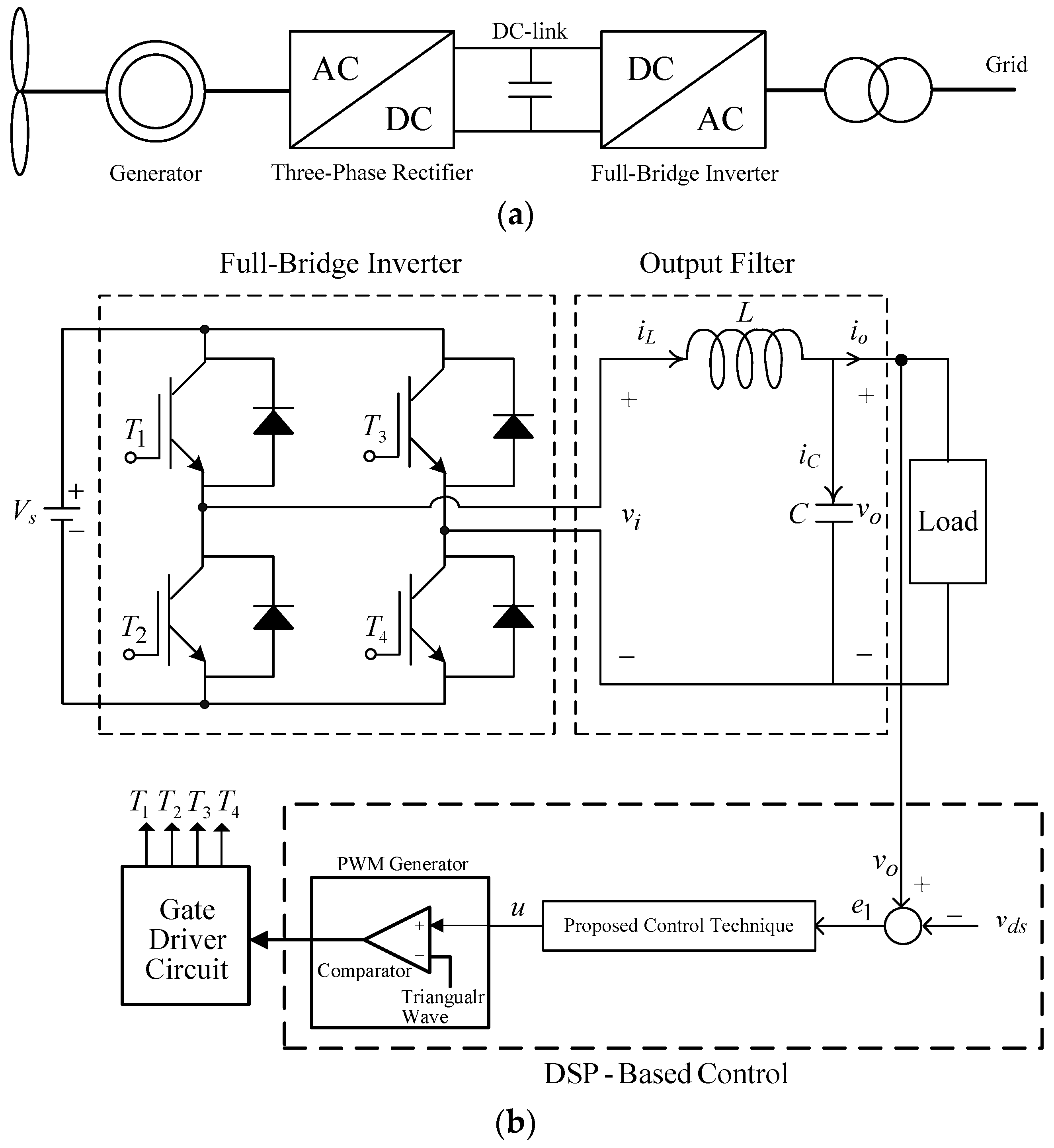
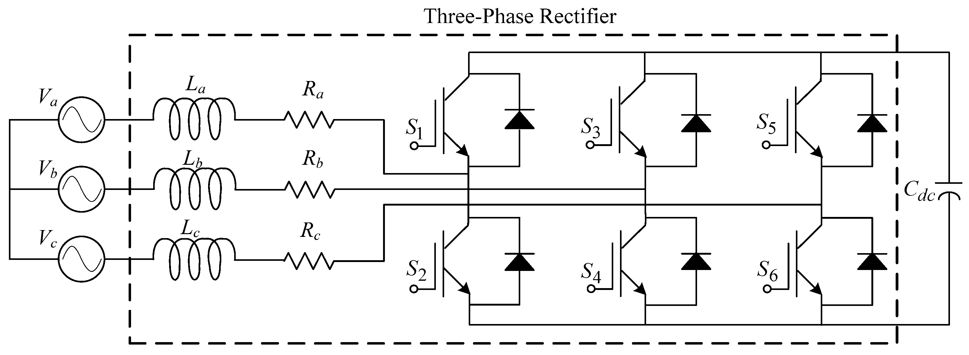
A wind energy conversion system is sketched in Figure 1a. It is composed of a wind generator (which can be a synchronous generator, a permanent-magnet synchronous generator, or a doubly-fed induction generator), three-phase rectifier, DC-link capacitor, full-bridge inverter, and the grid. The AC output voltage of the wind generator is transformed into DC voltage by the use of a rectifier circuit; then, the DC voltage using the inverter circuit is transformed into AC electrical power with constant voltage and frequency to the power grid. It is noteworthy that a small wind power system employs a three-phase generator, but it is frequently connected to a single-phase power distribution system. Thereby, a single-phase full-bridge inverter must provide low THD sinusoidal output voltage and a fast transient response. Figure 1b shows the circuit diagram of a full-bridge inverter followed by an LC (inductor-capacitor) filter and load. The use of the second-order LC filter can remove the high-frequency component of the output voltage v_i. The DC bus voltage $V_s$ can be regarded as an ideal constant voltage supply, $v_0$ denotes the output voltage, $i_0$ symbols the output current, and $L$, $C$, and $R$ are the inductor, capacitor, and load, respectively. The output voltage is desired to be maintained as close as possible to a sinusoidal reference waveform even under highly nonlinear loading. By choosing the state variables as $x_1=v_0$ and $x_2={\dot{v}}_0$, the dynamics of the full-bridge inverter in a state-space representation can be expressed as follows:

$$\left[\begin{array}{c}{\dot{x}}_1\\ {\dot{x}}_2\end{array}\right]=\left[\begin{array}{cc}0& 1\\ -1/LC& -1/RC\end{array}\right]\left[\begin{array}{c}{x}_1\\ x_2\end{array}\right]+\left[\begin{array}{c}0\\ K_{pwm}/LC\end{array}\right]u$$

(1)

where $u$ symbols the control signal. In the PWM (pulse width modulation) method [35], we suppose the switching frequency to be much greater than the fundamental frequency sine wave of 60 Hz. The PWM method will treat $K_{pwm}$ as a proportional gain of a PWM full-bridge inverter and is equal to $V_s/{\widehat{v}}_t$; here, ${\widehat{v}}_t$ is the amplitude of the triangular wave. The $u$ must be compared to $v_t$, producing the PWM signals, which controls the firing of the inverter switches. By the theory of state-space averaging [36], the output voltage $v_i$ equals the product of $u$ and $K_{pwm}$.

Figure 1. (a) Block diagram of a wind energy conversion system; (b) Full-bridge inverter and its controller.

The objective of the control is to find a control law so that the $v_0$ can track the desired sinusoidal waveform $v_{ds}(t)=V_m\sin (\omega t)$ in which $V_m$ and $\omega$ are the peak voltage and the angular frequency, respectively. The design of a full-bridge inverter can be regarded as a path-tracking control problem. Define the error state variables as:

$$e_1(t)=x_1(t)-v_{ds}(t)$$

(2)

$$e_2(t)={\dot{x}}_1(t)-{\dot{v}}_{ds}(t)=x_2(t)-{\dot{v}}_{ds}(t).$$

(3)

From Equations (1)–(3), the error state equations of a full-bridge inverter are derived as:

$$\{\begin{array}{l}{\dot{e}}_1(t)=e_2(t)\\ \\ {\dot{e}}_2(t)=-a_{w1}{e}_1(t)-a_{w2}{e}_2(t)+b_{w}u(t)-\phi (t)\end{array}$$

(4)

where $a_{w1}=1/LC$, $a_{w2}=1/RC$, $b_w=K_{pwm}/LC$, and $\phi =a_{w1}{v}_{ds}+a_{w2}{\dot{v}}_{ds}+{\ddot{v}}_{ds}$ is the uncertain disturbance.

As can be seen in system dynamics Equation (4), the load of the full-bridge inverter is changeable (i.e., can be many types). Under linear load conditions, the finite-time convergent SMGL can provide a high tracking accuracy of the steady-state performance and has fast finite-time convergence of error dynamics. Once the load is a large step change or an uncertainty or even a severe nonlinear condition, the finite-time convergent SMGL will yield a chatter/steady-state error and display a high THD. Thus, we develop the FNGBM-compensated finite-time convergent SMGL to resolve the chatter/steady state error problems, improving the performance of the transience and steady state for a full-bridge inverter.

3. Design of Control Technique

First, it is necessary to define the sliding surface of the classical finite-time convergent SMGL:

$$s=e_2+\beta e_1^{h/g}$$

(5)

where $\beta >0$, $g>h>0$ and $g$, $h$ are positive odd numbers. A sliding mode control law of the form can be used as $u=u^{+}$, $u^{-}$ for $s>0$, $s<0$, respectively, and then the $s$ can be impelled to the sliding mode $s=0$ within a finite time. The dynamics in Equation (5) yield $e_2={\dot{e}}_1=-\beta e_1^{h/g}$. While the initial state $e_1(0)\ne 0$ at $t=0$ is given, the dynamics will arrive at $e_1=0$ in a finite time determined by the relaxation time $t_1=g{\left|e_1(0)\right|}^{(g-h)/g}/\beta (g-h)$; this implies that in the finite-time convergent sliding mode, the convergence of the system state $e_1$ to the equilibrium point is reached in a finite time and then the convergence of the system state $e_2$ to the equilibrium point will be reached in finite time, too. Owing to $e_1$ and $e_2$ converged to the equilibrium point within a finite time, the $s$ given in Equation (5) also converges to zero within a finite time. Define the Jacobian matrix $J$ and then the finite-time convergent SMGL can be explained that around the equilibrium point $e_1=0$, the finite-time convergence of the system states to the equilibrium point is as follows: $J=\partial {\dot{e}}_1/\partial e_1=-\beta h/g{e}_1{}^{(g-h)/h}$; an eigenvalue of the first-order approximation matrix becomes ${J|}_{e_1\to 0^{+}}\to -\infty$. This tells us that at the equilibrium point the eigenvalue is prone to negative infinity and because of the infinitely negative eigenvalue, the system trajectory with an infinitely large speed will converge to the equilibrium point that leads to finite-time reachability.

The control law $u$ is thereby designed as:

$$u(t)=u_{eq}(t)+u_{sm}(t)$$

(6)

with:

$$u_{eq}(t)=b_w^{-1}[a_{w1}{e}_1+a_{w2}{e}_2-(\beta \cdot \frac{h}{g}{e}_1^{h/g-1}\cdot e_2)]$$

(7)

$$u_{sm}(t)=-b_w^{-1}\left[(\delta +\xi )\mathrm{sgn}(s)\right]$$

(8)

where $\delta \ge \left|\phi \right|$, $\delta >0$, $\xi >0$ and the $u_{eq}$ stands for the equivalent control in the face of an unperturbed plant, obtaining $s=0$ and $\dot{s}=0$. The $u_{sm}$ represents the sliding control for repressing the uncertain disturbances. Therefore, the system can reach the sliding mode $s=0$ and converge within a finite time. But, while $e_1$ passes through zero at a certain point in time, owing to $0<h/g<1$ and $e_1^{h/g-1}$, the singularity, which makes control law tend to infinity, yields and then leads to the instability of the closed-loop system.

To obtain singularity-free and finite system state convergence time, we redefine the sliding surface of the proposed finite-time convergent SMGL as:

$$s=e_1+\frac{1}{\beta }{e}_2^{g/h}$$

(9)

where $g>h$, $g$ and $h$ are positive odd numbers ($1<g/h<2$), and a sliding-mode reaching term $\dot{s}=-K{\left|s\right|}^{\alpha }\mathrm{sgn}(s)$ is created.

Then, the control law $u$ can be rewritten as:

$$u(t)=u_{neq}(t)+u_{fts}(t)$$

(10)

with:

$$u_{neq}(t)=b_w^{-1}[a_{w1}{x}_1+a_{w2}{e}_2-\beta \cdot \frac{h}{g}{e}_2^{2-g/h}]$$

(11)

$$u_{fts}(t)=-b_w^{-1}\left[K{\left|s\right|}^{\alpha }\mathrm{sgn}(s)\right]$$

(12)

where $K>0$, $0<\alpha <1$, $u_{neq}$ signifies the equivalent control with singularity-free, and $u_{fts}$ can repress plant parameter deviations and disturbances to guarantee the existence of a sliding mode.

Proof: Define Lyapunov-candidate function as:

$$V=\frac{1}{2}{s}^2.$$

(13)

Then, taking the derivative of $V$ along the trajectory of the dynamic system (Equation (4)) with the control law (Equation (10)) and using Equation (9), one yields:

$$\begin{array}{ll}\dot{V}& =s\dot{s}\\ & =s\left({\dot{e}}_1+\frac{1}{\beta }\frac{g}{h}{e}_2^{g/h-1}{\dot{e}}_2\right)\\ & \le -s\left(\frac{1}{\beta }\frac{g}{h}{e}_2^{g/h-1}(K{\left|s\right|}^{\alpha }\mathrm{sgn}(s)\right)\\ & \le 0\end{array}.$$

(14)

Equation (14) means that Equation (9) and the system states Equation (4) can converge to the equilibrium point in finite time. Note that if the load is a highly nonlinear condition, the finite-time convergent SMGL will produce chatter or steady-state error, thus incurring inexact tracking behavior in the full-bridge inverter design; that is, the output voltage $v_0$ does not track a reference voltage $v_{ds}$ completely and the difference measure between $v_0$ and $v_{ds}$ cannot converge to zero. Thus, the control signal $u(t)$ (Equation (10)) is modified by the addition of an FNGBM compensator ($u_{fgb}(t)$), which reduces the chatter/steady-state error in the full-bridge inverter. The modeling steps of the FNGBM are described below.

• Step 1: Input the original sample data sequence

Let the original data sequence be denoted as:

$$x_{}^{(0)}=\left\{x_{}^{(0)}(k),k=1,2,\dots ,n\right\}$$

(15)

where $x^{(0)}$ stands for the set of $n$ original sample data.

• Step 2: Accumulated generating operation (AGO)

By taking the AGO on $x_{}^{(0)}$, the first-order AGO sequence can be written as:

$$X_{}^{(1)}=\left\{{\displaystyle \sum _{i=1}^1{x}_{}^{(0)}(i)},{\displaystyle \sum _{i=1}^2{x}_{}^{(0)}(i)},\dots ,{\displaystyle \sum _{i=1}^k{x}_{}^{(0)}(i)}\right\},k=1,2,\dots ,n.$$

(16)

• Step 3: Construct the grey differential equation of NGBM(1,1) as:

$$x_{}^{(0)}(k)+a{z}^{(1)}(k)=b{[z^{(1)}(k)]}^{\gamma }.$$

(17)

Also, the whitenization differential equation is expressed as:

$$\frac{d{x}^{(1)}}{dt}+a{x}_{}^{(1)}=b{[x^{(1)}]}^{\gamma }$$

(18)

where $z_{}^{(1)}(k)=p{x}^{(1)}(k)+(1-p)x^{(1)}(k-1)$, $k=2,3,\dots ,n$, $p\in [0,1]$ represents the generating coefficient of the background value and $\gamma$ belongs to any real number precluding $\gamma =1$.

• Step 4: Solve the estimated parameters $a$ and $b$ by the least square method below.

$$\left[a,b\right]={(N^{T}N)}^{-1}{N}^{T}M$$

(19)

where:

$$N=\left[\begin{array}{cc}-z{x}_{}^{(1)}(2)& {[z{x}_{}^{(1)}(2)]}^{\gamma }\\ -z{x}_{}^{(1)}(3)& {[z{x}_{}^{(1)}(3)]}^{\gamma }\\ ⋮& ⋮\\ -z{x}_{}^{(1)}(n)& {[z{x}_{}^{(1)}(n)]}^{\gamma }\end{array}\right]\mathrm{and}M=\left[\begin{array}{c}{x}_{}^{(0)}(2)\\ x_{}^{(0)}(3)\\ ⋮\\ x_{}^{(0)}(n)\end{array}\right].$$

• Step 5: The solution of Equation (18) yields:

$${\widehat{x}}_{}^{(1)}(k)={[(x_{}^{(1)}{(1)}^{1-\gamma }-\frac{b}{a})e^{-a(1-\gamma )(k-1)}+\frac{b}{a}]}^{1/1-\gamma },\gamma \ne 1,k=1,2,\dots ,n$$

(20)

where ‘^’ denotes the forecasted value.

• Step 6: Inverse accumulated generating operation (IAGO)

By using IAGO, the data sequence ${\widehat{x}}_{}^{(0)}(k)$ can be estimated as:

$${\widehat{x}}^{(0)}(1)=x^{(0)}(1)$$

(21)

$${\widehat{x}}_{}^{(0)}(k)={\widehat{x}}^{(1)}(k)-{\widehat{x}}^{(1)}(k-1),k=2,3,\dots ,n.$$

(22)

To improve the accuracy of the forecasting models, the Fourier series is used in modifying the residuals in NGBM(1,1) so that a Fourier nonlinear grey Bernoulli model (FNGBM(1,1)) can be obtained.

• Step 7: Get the residual series from NGBM(1,1)

Based on the forecasted series $v_r$, a residual series ${\epsilon }_r$ can be represented as:

$${\epsilon }_r=\left\{{\epsilon }_r(2),{\epsilon }_r(3),\dots ,{\epsilon }_r(n)\right\}$$

(23)

where ${\epsilon }_r(k)=x(k)-v_r(k)$.

• Step 8: Define FNGBM(1,1)

The ${\epsilon }_r$ can be approximated through a Fourier series in the following:

$${\epsilon }_r=\frac{1}{2}{a}_0+{\displaystyle \sum _{i=1}^z[a_i}\cos (\frac{2\pi i}{n-1}k)+b_i\sin (\frac{2\pi i}{n-1}k)]$$

(24)

where $k=2,3,\dots ,n$, and $z=(\frac{n-1}{2})-1$.

Thus, the residual series is restated as:

$${\epsilon }_r=P{C}_r$$

(25)

where $P=\left[\begin{array}{cccccc}\frac{1}{2}& \cos (\frac{2\pi \cdot 1}{n-1}\cdot 2)& \sin (\frac{2\pi \cdot 1}{n-1}\cdot 2)& \cdots & \cos (\frac{2\pi \cdot z}{n-1}\cdot 2)& \sin (\frac{2\pi \cdot z}{n-1}\cdot 2)\\ \frac{1}{2}& \cos (\frac{2\pi \cdot 1}{n-1}\cdot 3)& \sin (\frac{2\pi \cdot 1}{n-1}\cdot 3)& \cdots & \cos (\frac{2\pi \cdot z}{n-1}\cdot 3)& \sin (\frac{2\pi \cdot z}{n-1}\cdot 3)\\ ⋮& ⋮& ⋮& ⋮& ⋮& ⋮\\ \frac{1}{2}& \cos (\frac{2\pi \cdot 1}{n-1}\cdot n)& \sin (\frac{2\pi \cdot 1}{n-1}\cdot n)& \cdots & \cos (\frac{2\pi \cdot z}{n-1}\cdot n)& \sin (\frac{2\pi \cdot z}{n-1}\cdot n)\end{array}\right]$ and $C_r={[a_0,a_1,b_1,a_2,b_2,\dots ,a_z,b_z]}^T$.

By using the least squares method, the parameters $a_0,a_1,b_1,a_2,b_2,\dots ,a_z,b_z$ can be obtained as:

$$C_r={(P^{T}P)}^{-1}{P}^T{\epsilon }_r{}^T.$$

(26)

Once these parameters are computed, the modified residual series is performed as:

$${\widehat{\epsilon }}_r=\frac{1}{2}{a}_0+{\displaystyle \sum _{i=1}^z[a_i}\cos (\frac{2\pi i}{n-1}k)+b_i\sin (\frac{2\pi i}{n-1}k)].$$

(27)

• Step 9: Correct forecast series

From the forecast series $v_r$ and ${\epsilon }_r$, the Fourier modified series ${\widehat{v}}_r$ of series $v_r$ can be decided as:

$$v_r=\left\{{\widehat{v}}_{r1},{\widehat{v}}_{r2},{\widehat{v}}_{r3},\dots ,{\widehat{v}}_{rk},\dots ,{\widehat{v}}_{rn}\right\}$$

(28)

where:

$${\widehat{v}}_r=\{\begin{array}{c}{\widehat{v}}_r=v_r\hfill \\ {\widehat{v}}_{rk}=v_{rk}+{\widehat{\epsilon }}_{rk},k=2,3,\dots ,n\hfill \end{array}.$$

(29)

Thereby, the control law of Equation (10) is rewritten as:

$$u=u_{neq}+u_{fts}+u_{fgb}$$

(30)

where the following $u_{fgb}$ stands for Fourier modified NGBM for lessening the chatter/steady-state error:

$$u_{fgb}=\{\begin{array}{c}0,\\ \mathsf{\Psi }\widehat{s}\mathrm{sgn}(s\widehat{s}),\end{array}\begin{array}{c}\left|\widehat{s}\right|<\kappa \\ \left|\widehat{s}\right|\ge \kappa \end{array}$$

(31)

where $\widehat{s}$ indicates the forecasted value of $s$, $\mathsf{\Psi }$ is a constant, and $\kappa$ symbols the system boundary. The control law $u$ Equation (10) of the finite-time convergent SMGL is made up of $u_{neq}$ and $u_{fts}$. The $u_{neq}$ is identical to the proposed control technique in Equation (30). However, the parameter $K$ of $u_{fts}$ is bigger than or equal to the perturbation $\left|\phi \right|$. The $u_{fts}$ in Equation (10) is substituted by $u_{fts}$ and $u_{fgb}$ as shown in Equation (30). If the maximum uncertain system boundary is identified, there is the same performance in the proposed control technique and the finite-time convergent SMGL. Once the maximum uncertain system boundary is unidentified, a restrained feedback gain yields severe chatter in the finite-time convergent SMGL. To attenuate the chatter occurred in $u_{fts}$, the restrained feedback gain in Equation (30) of the proposed control technique is separated into two parts, $u_{fts}$ and $u_{fgb}$. While the $\left|s\right|$ exceeds boundary layer width $\kappa$, $u_{fgb}$ designed in Equation (30) is acted on such circumstance, thus yielding the reduction of the chattering.

4. Simulation and Experimental Results

The potential of the proposed full-bridge inverter is verified by simulations and experiments. The nominal values of the full-bridge inverter parameters used for the proposed control technique are listed in Table 1.

Table 1. Nominal parameters for the full-bridge inverter.

Output Voltage, ${\mathit{v}}_0$	110 Vrms
DC source voltage, $V_s$	210 V
Output voltage frequency, $f_0$	60 Hz
Switching frequency, $f_s$	18 kHz
Resistive load, $R$	12 Ω
Filter inductor, $L$	0.2 mH
Filter capacitor, $C$	3 μF

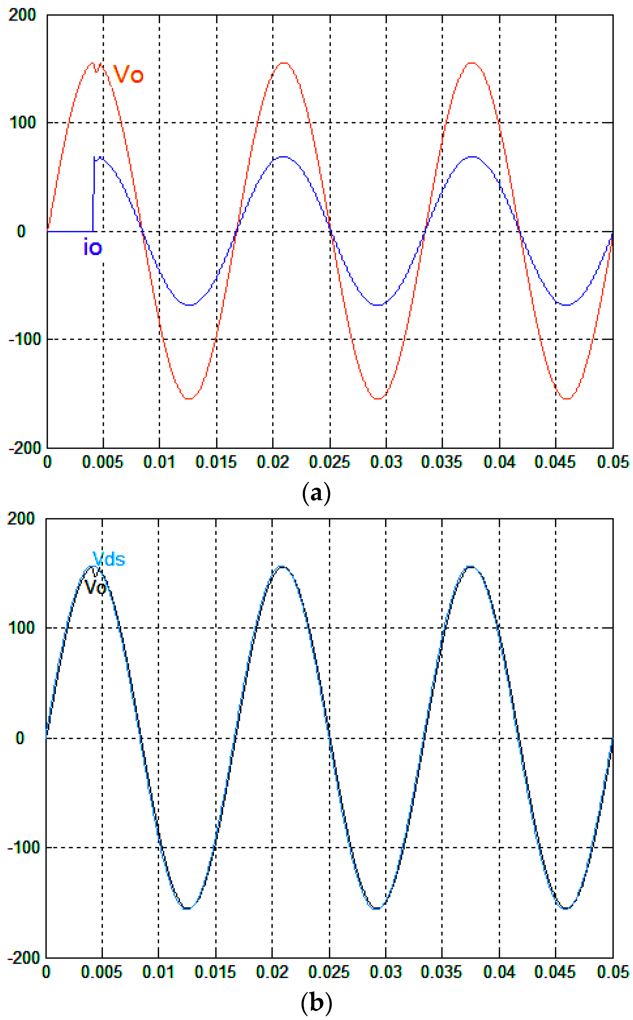
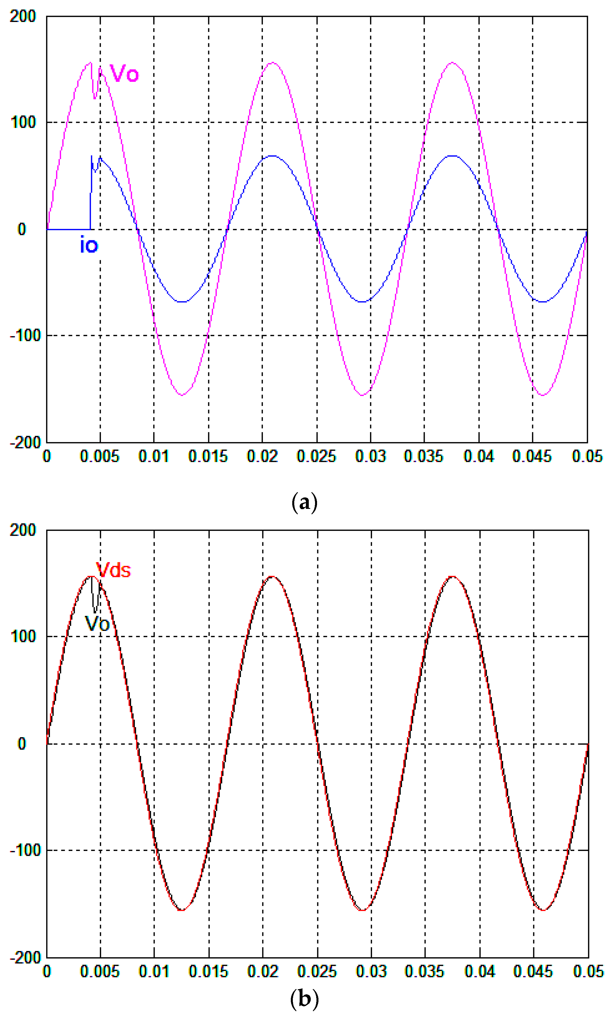
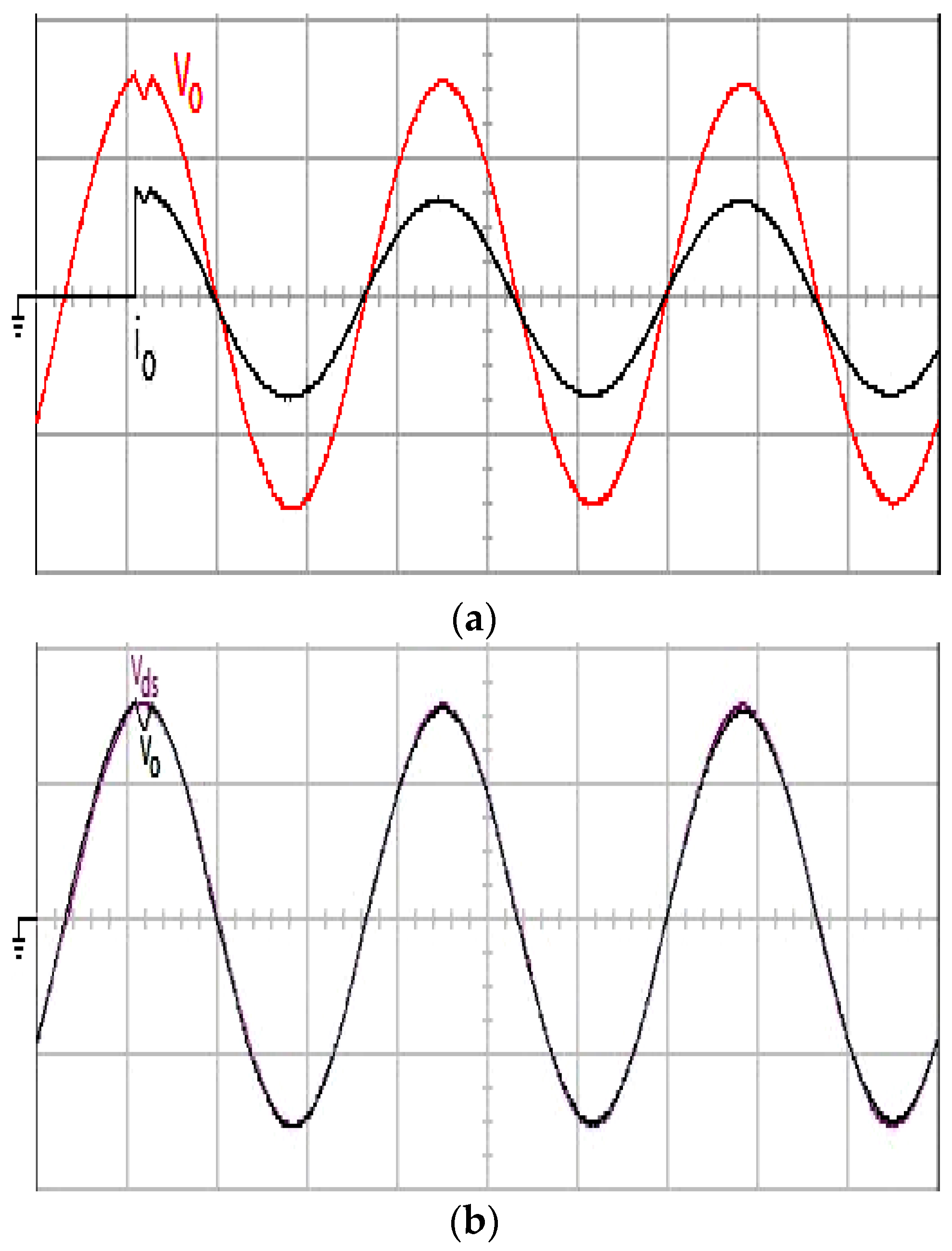
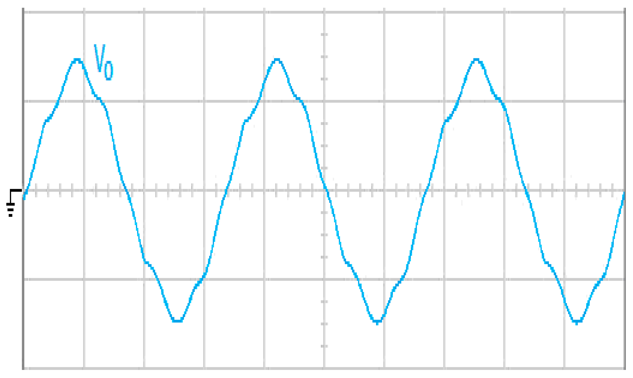
Figure 2a and Figure 3a show the simulated waveforms for the proposed control technique and the classical finite-time convergent SMGL under step load change from no load to full load, respectively. The output voltage of the proposed controlled full-bridge inverter shown in Figure 2a exhibits smaller instant sag and a higher tracking accuracy than that of the classical finite-time convergent SMGL-controlled full-bridge inverter shown in Figure 3a. Because the classical finite-time convergent SMGL does not hit the sliding surface accurately, the chatter/steady-state error occurs under such difficult test conditions (step load change); relatively, the proposed control technique due to FNGBM compensation can reduce the chatter/steady-state error, thus leading to fast transience. The requested output voltage with the proposed control technique recovers from a small transience with about 6 V_rms voltage sag, but the classical finite-time convergent SMGL-controlled full-bridge inverter has a severe 24 V_rms voltage sag. 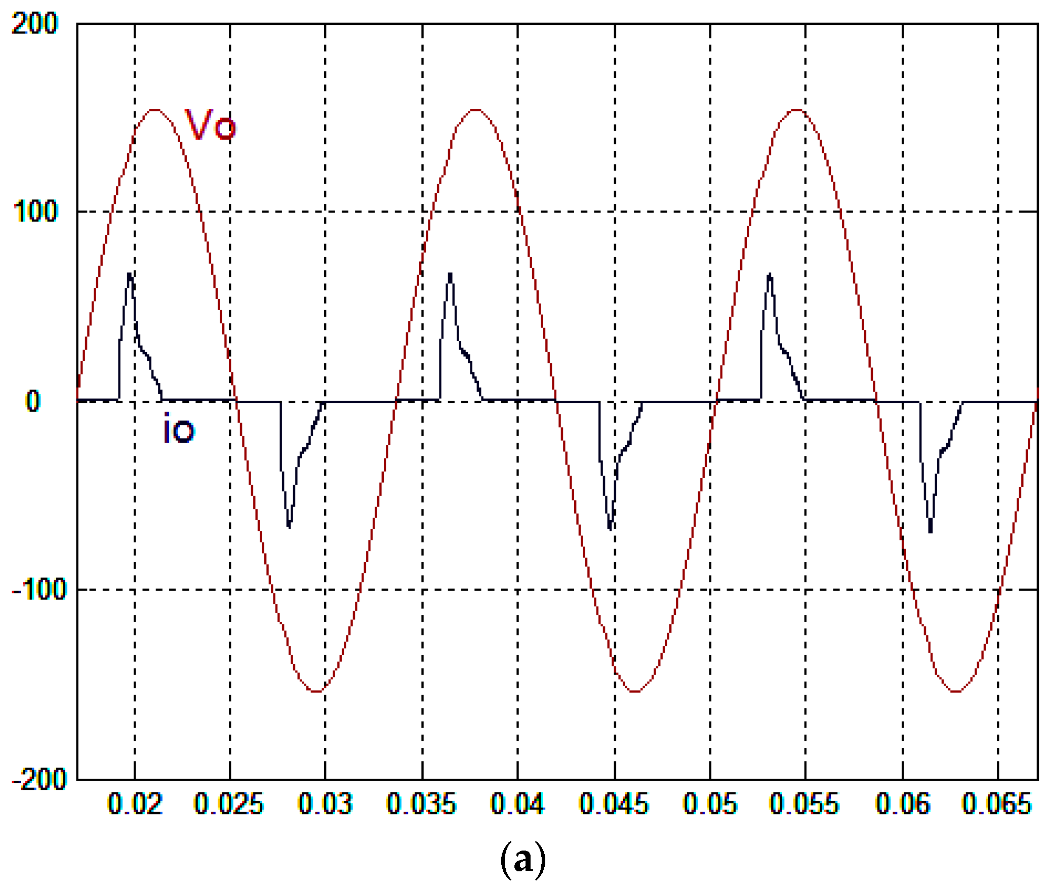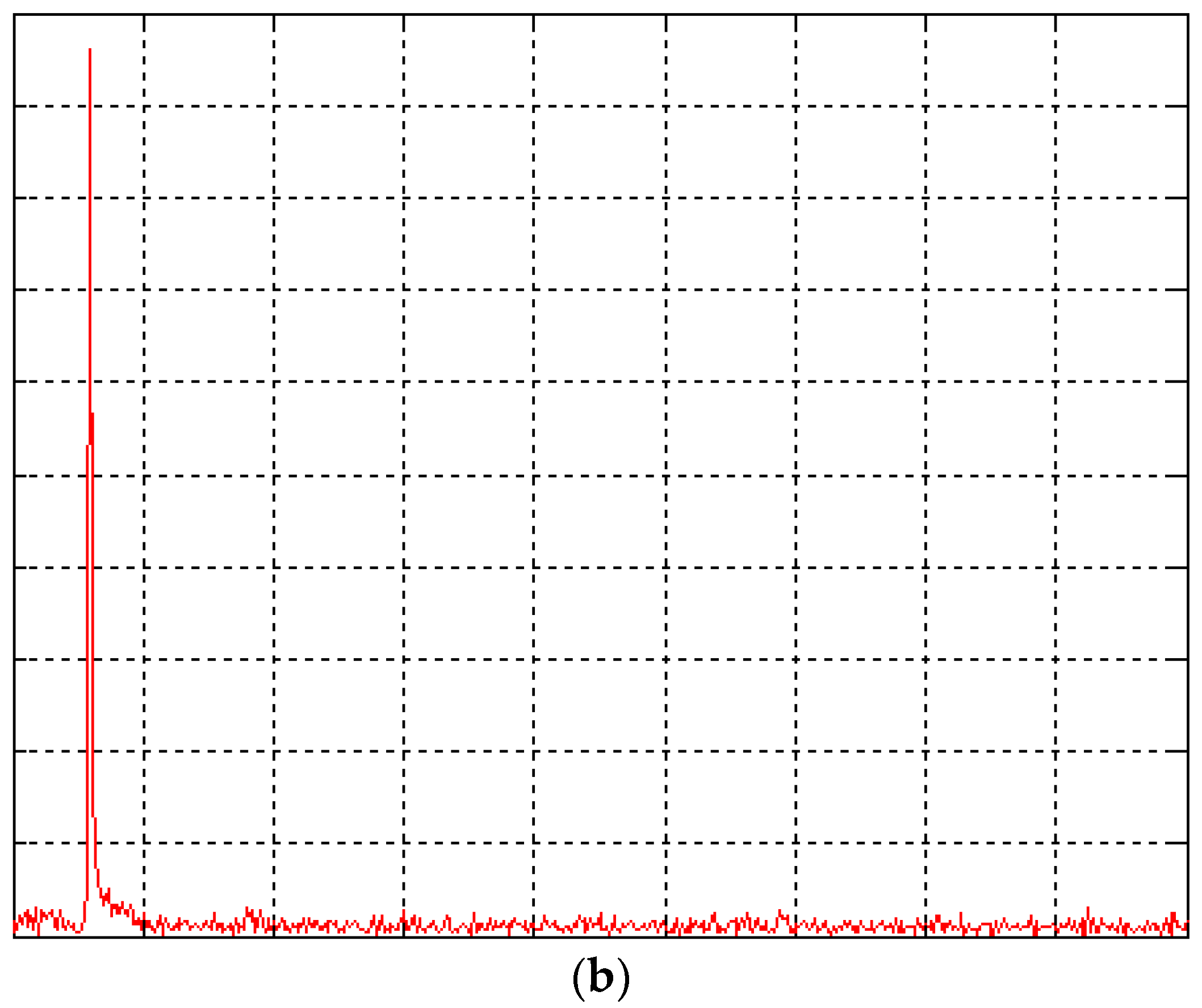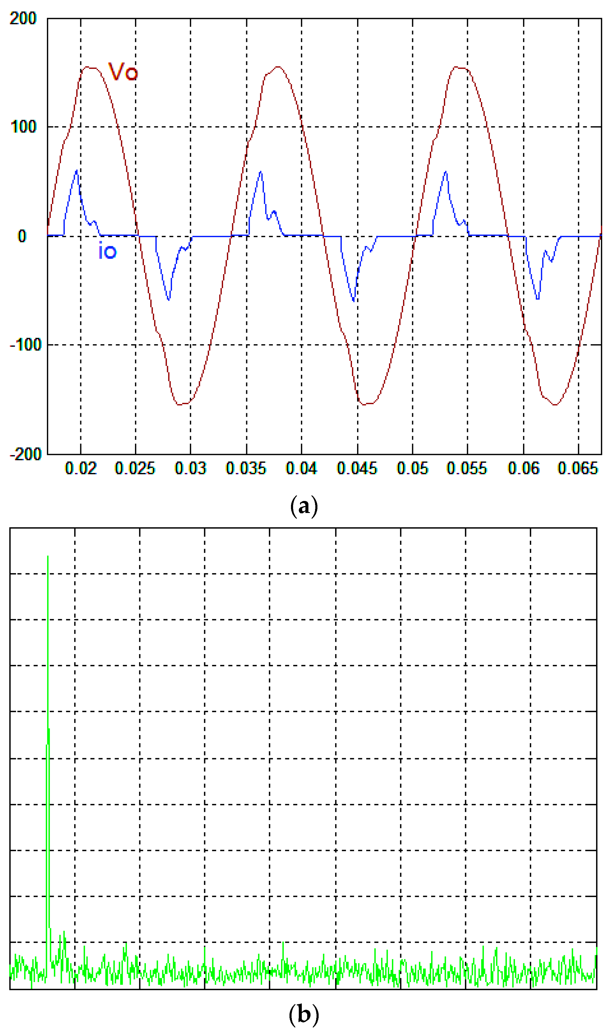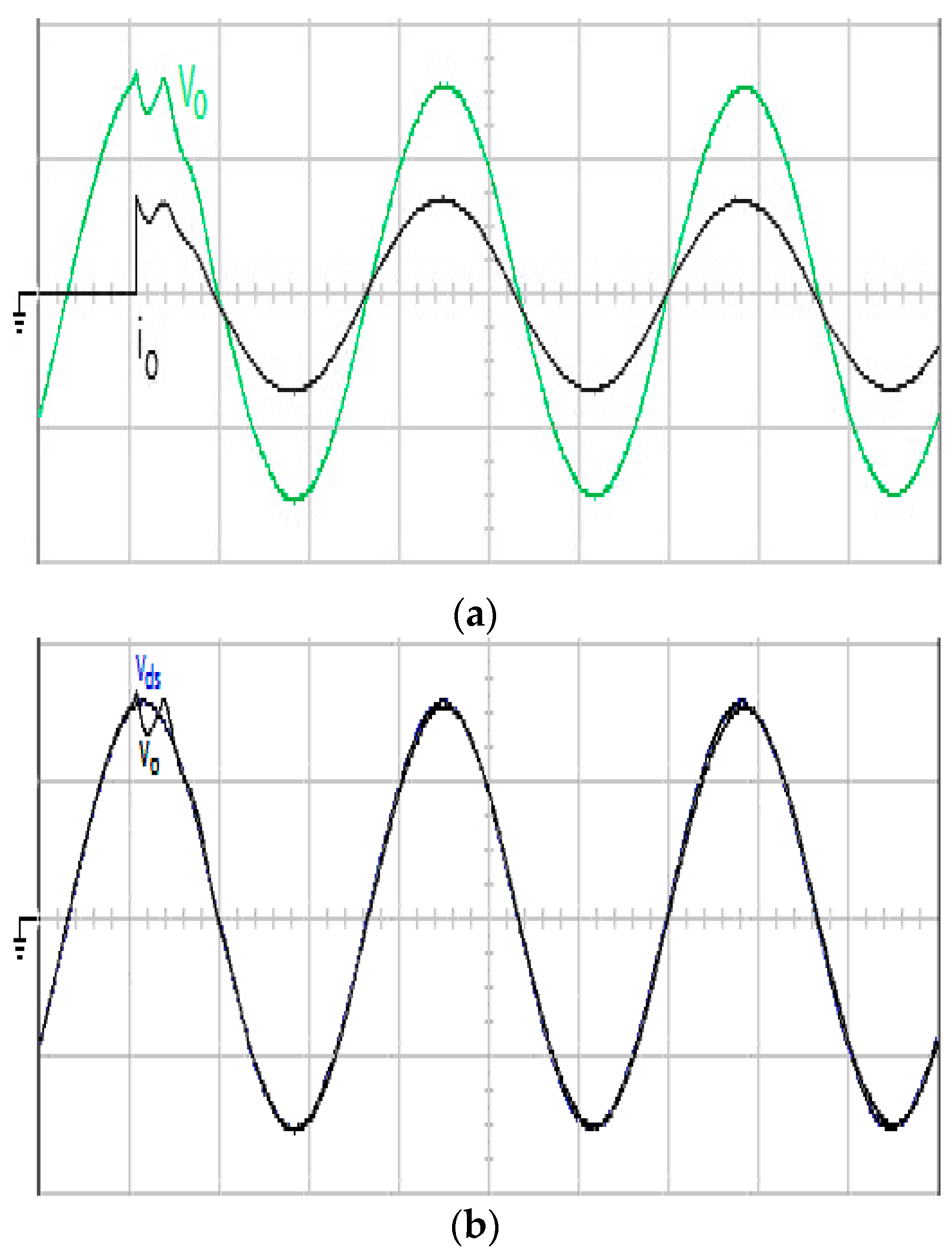Both Figure 2b and Figure 3b plot the trajectories of the output voltage and reference sine wave to examine the tracking error. The performance of the full-bridge inverter for the proposed control technique under severe nonlinear loading, which consisted of a full-wave diode bridge rectifier with an electrolytic capacitor of 220 μF and a load resistance of 35 Ω to simulate the waveforms, is reported in Figure 4a. Although the output current has high distortion, the output voltage is almost a sinusoidal waveform, has good steady-state exactness, and provides low voltage THD (%THD equals 1.75%). Compared with the proposed control technique, the simulated waveforms for the classical finite-time convergent SMGL under the same load are shown in Figure 5a with a high voltage %THD of 10.56%, and thus incurring unsatisfactory steady-state exactness. The harmonic spectra are shown in Figure 4b and Figure 5b to show the differences in terms of THD. Figure 6a shows the experimental waveform for the proposed control technique under step load change from no load to full load. Note that the transient behavior is good (small voltage sag) and after the transience, the voltage waveform returns to precision sinusoidal tracking. However, the experimental waveform for the classical finite-time convergent SMGL, shown in Figure 7a, has a significant voltage sag and a slow recovery time at the firing angle. Notice that owing to the compensation of the FNGBM, the output voltage with the proposed control technique arrives at the requested value behind the 11 V_rms voltage sag. On the contrary, after a 20 V_rms voltage sag, the output voltage with the classical finite-time convergent SMGL shows an oscillatory tracking behavior near the firing angle. 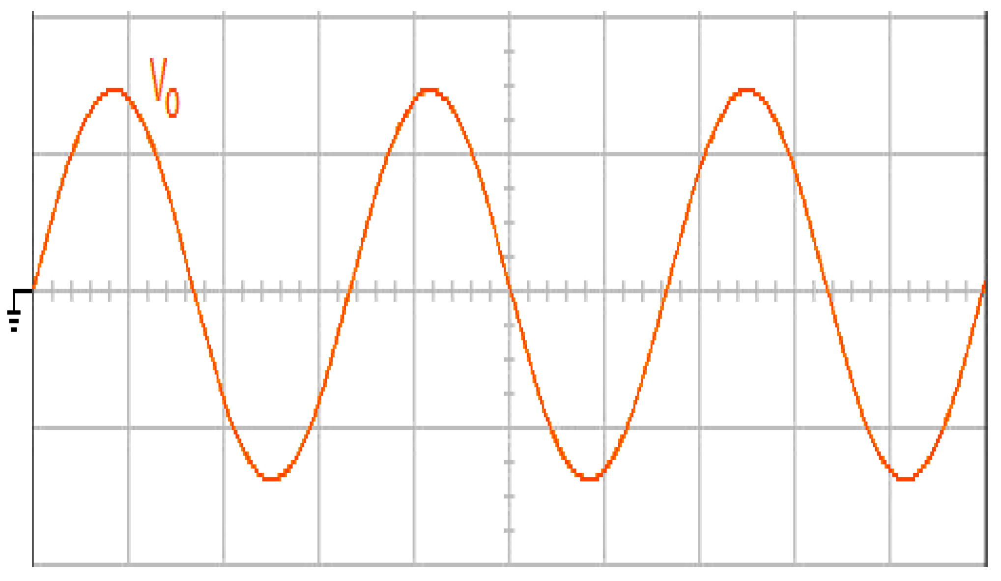The states’ trajectories in Figure 6b and Figure 7b are displayed for observing the tracking error. The system is applied with a random variation of filter parameters L and C from 10% to 100% of nominal values under resistive load 12 Ω; according to Figure 8, with the proposed control technique, the output voltage has not only a high output voltage exactness but also insensitivity to parameter variations, while the classical finite-time convergent SMGL, shown in Figure 9, represents a visible steady-state vibration with serious distortion. Table 2 compares the voltage sag and THD of the output voltage for the proposed control technique and the classical finite-time convergent SMGL. Both by simulated and experimental results, it is well verified that the proposed control technique due to the FNGBM compensation creates higher steady-state exactness, lower THD, and faster convergence under various load conditions.

Figure 2. (a) Simulation waveforms of the output voltage and output current under step load change for the proposed control technique (100 V/div; 20 A/div); (b) Trajectories of output voltage and reference sine wave.

Figure 3. (a) Simulation waveforms of the output voltage and output current under step load change for the classical finite-time convergent SMGL (100 V/div; 20 A/div); (b) Trajectories of output voltage and reference sine wave.

Figure 4. (a) Simulation waveforms of the output voltage and output current under nonlinear load for the proposed control technique (100 V/div; 20 A/div); (b) Harmonic spectrum of output voltage.

Figure 5. (a) Simulation waveforms of the output voltage and output current under nonlinear load for the classical finite-time convergent SMGL (100 V/div; 20 A/div); (b) Harmonic spectrum of output voltage.

Figure 6. (a) Experimental waveforms of the output voltage and output current under step load change for the proposed control technique (100 V/div; 20 A/div; 5 ms/div); (b) Trajectories of output voltage and reference sine wave (100 V/div; 5 ms/div).

Figure 7. (a) Experimental waveforms of the output voltage and output current under step load change for the classical finite-time convergent SMGL (100 V/div; 20 A/div; 5 ms/div); (b) Trajectories of output voltage and reference sine wave (100 V/div; 5 ms/div).

Figure 8. Experimental waveform of the output voltage under the variation of filter parameters L and C for the proposed control technique (100 V/div; 5 ms/div).

Figure 9. Experimental waveform of the output voltage under the variation of filter parameters L and C for the classical finite-time convergent SMGL (100 V/div; 5 ms/div).

Table 2. Voltage sag and percent total harmonic distortion (%THD).

Proposed Control Technique
Simulation	Voltage sag	%THD
	Step load change	Nonlinear load
	6 Vrms	1.75%
Classical Finite-Time Convergent SMGL
Simulation	Voltage sag	%THD
	Step load change	Nonlinear load
	24 Vrms	10.56%
Proposed Control Technique
Experiment	Voltage sag	%THD
	Step load change	LC variation
	11 Vrms	0.84%
Classical Finite-Time Convergent SMGL
Experiment	Voltage sag	%THD
	Step load change	LC variation
	20 Vrms	11.76%

5. Discussion and Future Research

For the sake of more advanced research in the future, the results can be discussed expansively and with comparison analysis to prior publications. For example, Figure 4 displays high harmonic voltage distortion, resulting in an unsatisfactory steady-state response that can be defended from earlier literature in the following: A continuous terminal sliding mode control based on system output and the estimations of its high-order derivatives is presented, as is its application to a DC-AC inverter. Even though the proposed controller guarantees system output converged to the equilibrium point within finite time, the steady-state error still appears in uncertain disturbances [37]. The integral action in a terminal sliding mode-controlled wind turbine system has been proposed. A large amount of the steady-state error has been decreased, but a fast dynamic response cannot be exhibited [38]. The high-order finite-time convergent sliding mode control with applications to wind energy systems is presented; however, the design of the algorithm is complicated and there is steady-state distortion in the presence of nonlinear loading [39]. The combination of the finite-time fast sliding mode and recursive structure has been developed to improve the performance of the inverter-based microgrid. This methodology has a chatter-free advantage but the state trajectory cannot meet the desired surface accurately, incurring serious voltage distortion and poor transient behavior [40]. Regarding the above-cited, the classical finite-time convergent SMGL-controlled inverter has inexact tracking in the steady-state and transient conditions. Thus, the proposed full-bridge inverter does produce an improved performance and can be combined with a three-phase high-power factor rectifier (as shown in Figure 10) to achieve a more complete wind energy conversion system in future research.

Figure 10. Future work with a three-phase rectifier integrated into the proposed full-bridge inverter.

6. Conclusions

In this paper, a finite-time convergent SMGL with FNGBM for full-bridge inverters has been developed, showing low THD under nonlinear load and fast dynamic response under step change in load. The characteristic of the FNGBM-compensated finite-time convergent SMGL over the SMC is fast convergence in finite time. When system uncertainty boundaries are overestimated or underestimated, the chatter/steady-state error occurs. The FNGBM is employed to lessen the chatter and steady-state error, thus achieving a more exact tracking performance. Simulation and experimental results on a full-bridge inverter prototype using a DSP have been reported to verify the applicability of the proposed control technique. We are confident that the proposed full-bridge inverter can be associated with wind-related circuits, such as three-phase AC-DC rectifier circuits and DC-DC converter circuits. These circuits will promote our further research work in the future.