Article

Solar Ray Tracing Analysis to Determine Energy Availability in a CPC Designed for Use as a Residential Water Heater

1
Renewable Energy Department, Centro de Investigación Científica de Yucatán, Mérida 97200, Mexico
2
Conacyt—Centro de Investigaciones en Óptica, Unidad de Aguascalientes, Prol. Constitución 607, Reserva Loma Bonita, Aguascalientes 20200, Mexico
3
Arian International Projects, c/Baldiri Reixach, 4, 08028 Barcelona, Spain
4
Metal-Mechanical Department, Instituto Tecnológico Nacional de México, Campus Apizaco, Av. Instituto Tecnológico S/N, Apizaco 90300, Mexico
*
Author to whom correspondence should be addressed.
Energies 2018, 11(2), 291; https://doi.org/10.3390/en11020291
Submission received: 24 November 2017 / Revised: 22 December 2017 / Accepted: 28 December 2017 / Published: 25 January 2018

Abstract

:
Compound parabolic concentrators are relevant systems used in solar thermal technology. With adequate tailoring, they can be used as an efficient and low-cost alternative in residential water heating applications. This work presents a simulation study using a ray tracing analysis. With this technique, we simulate the interaction between solar rays and solar concentrator to quantify the amount of energy that impinges on the receiver at a particular time. Energy availability is evaluated in a comparison of two configurations throughout the year: static setup at 21° and multi-position setup; tilted with respect to the horizontal, depending on three seasonal positions: 0° for summer, 16° for spring/autumn, and 32° for winter, with the aim to evaluate the amount of available energy in each season. The fact that a tracking system can be dispensed with also represents an economical option for the proposed application. The results showed that at 21°, the proposed solar Compound Parabolic Concentrator (CPC) works satisfactorily; however, by carrying out the selected angular adjustments, the overall energy availability increased by 22%, resulting in a more efficient option. The most effective design was also built and analyzed outdoors. The obtained thermal efficiency was of ~43%. The optical design and its evaluation developed herein proved to be a valuable tool for prototype design and performance evaluation.

1. Introduction

Compound Parabolic Solar Concentrators (CPCs) were described as a collector for cosmic light from Cherenkov counters by Hinterberger in Winston’s book [1]. CPCs are considered to be ideal concentrators, identified in the family of non-image concentrators. According to Kalogirou, CPC is classified as a medium temperature application (100–250 °C) [2,3]. The application, design, and geometrical parameters for solar concentrators with cylindrical receivers are described by Winston [1]. Rabl conducted a study to determine the optical and thermal properties of a CPC [4]. From this work, it was determined that the CPC is very close to be the ideal solar concentrator, because it reaches the highest concentration possible for any angle of acceptance [5,6]. This study also provides the formulae for calculating average reflections in a CPC. For an ideal CPC, only two parameters are required, acceptance angle and receiver diameter; in this way, these parameters define the concentrator’s width and height [7]. A CPC usually requires few or no adjustments to its angular position, for example, throughout a typical seasonal year [7,8,9,10,11]. A CPC system usually has construction imperfections that impact its efficiency; therefore, a common task is to minimize losses by taking into account the restrictions imposed by the design, material properties, and cost considerations [8,12,13]. In this manner, the quality of the optical properties and the shape of the reflecting surface of a concentrator determine the level of concentration that the receiver can reach. The deviations from the ideal performance are due to optical errors of the concentrator [14,15]. These can be classified into two types: First, the shape of the surface of the concentrator, the closer it is to the ideal, the smaller the error will be; this error is commonly called contour error. The second is the error produced by the specular reflection of the material; this error is mainly due to surface roughness, i.e., surface imperfections at microscale [16].
In this type of collector, the lack of solar radiation on the lower part of the receiver can be resolved by matching the acceptance angle of the concentrator with the solar vector, thereby obtaining a more homogeneous impinging of the sun’s rays on the concentrator. It is important to consider that a uniform solar illumination of the receiver area is desired, due to the intense radiation generated by the concentration effect. If there are deformations or manufacturing defects on the concentrator surface (or misalignment), radiation hot spots will be promoted, giving an uneven distribution of heat on the receiver. These types of errors can be ignored for a high conductivity receiver, but practical systems require the minimization of this issue if proper heat transfer is desired [16,17,18].
A solar concentrator depends greatly on its focal alignment, thus, in static systems, a significant loss in energy availability can occur [1]. Ray tracing software is a very useful tool, since it allows the user to estimate the amount and distribution of concentrated solar energy that the receiver is capable of transmitting at any moment, defining geometry and construction materials. For example, in 2010, Colina-Marquez et al. used a solar tracing software tool to determine energy distribution on a receiver, testing three reflective surfaces [19]. In 2014, Chia-Wei et al. [20] proposed a modification in the positioning of the receiver, varying the focal point from the relationship between height and diameter, and found that the optimal ratio between them was 0.46; the angle of incidence from 1.5 to 6 degrees was also evaluated using a ray tracing analysis to estimate the amount of concentrated energy in the receiver. In the same year, Waghmare et al. presented a ray tracing-based analysis, which analyzed the effect of limiting the diameter of the receiver in order to reduce optical losses [21]. Yurchenko et al. established a ray tracing analysis for the optical and thermal optimization of a CPC, resulting in the use of a configuration of V vents with which an optimal value was obtained for the positioning of these in the receiver for a typical CPC [8]. In 2015, Lin et al. analyzed a two-dimensional CPC with a tubular receiver, varying the collector’s profile and truncating the reflector to a lower height; the CPC was seasonal tilted and was oriented to east–west. Using the ray tracing method, a numerical model was developed to study the performance of the modified collector [22]. In 2016, Bellos et al. applied the use of a ray tracing tool combined with finite element analysis to optimize a CPC design from optical and thermal performance [23].
This work proposes to study the use of a CPC in a lower temperature range (40–60 °C) as a residential solar heater, taking advantage of the greater efficiency provided by the system for a given temperature. In this collector type, the opening area of the CPC is more reduced than other systems, such as flat plate heater (FPH), combined with the use of high reflective surface and the geometry of the concentrator, allowing concentrating more energy in the receiver. In this sense, the dimensions of the CPC system can be more reduced (and lighter), decreasing the material used. In addition to this, it has been quantified that the parts used for a FPH are more than those used in a CPC; therefore, the use of less material and less assembly time opens an opportunity window to evaluate the potential use of CPCs for residential applications.
To achieve this, the study proposes the dimensioning of a CPC system that operates in a low temperature range (40 to 60 °C), using a ray tracing software to determine the energy availability in two scenarios, static and multi-position setups [23,24]. The analysis for this particular work was carried out in the geographic location of Merida, Mexico; however, it could be used in any region of interest. In addition to the optical study, the construction and instrumentation of an experimental prototype was carried out in order to evaluate the proposed system in real conditions.

2. Materials and Methods

2.1. Concentrator Ratio

The concentration ratio, CR, together with the receiver diameter, represent the basic parameters for a CPC design. For the CR, the relative movement of the sun in the celestial vault throughout the year (Analemma) is taken into account, and the calculation is carried out with reference to the solar noon θz using the equations proposed by Duffie et al. [5]. For the coordinates of this study (21.02° N, −89.63° W), the summer solstice, the maximum angle of the sun is −4.27°, taking as a reference the vertical (Y axis), whereas in the winter solstice, the maximum angle reached is 42.16°.
It is well known that a high concentration factor gathers more energy; however, this entails the need for more periodical adjustments during the day to capture solar rays. Based on this, and taking into consideration the solar trajectory in the celestial vault, in order to reduce the loss of solar incidence throughout the year, a concentrator acceptance angle of 45° was selected.
Before calculating the available energy at the receiver and in order to facilitate a better understanding of the results of solar ray trace campaign, the concentrator acceptance angle aligned with β (inclination angle of CPC) was evaluated. 
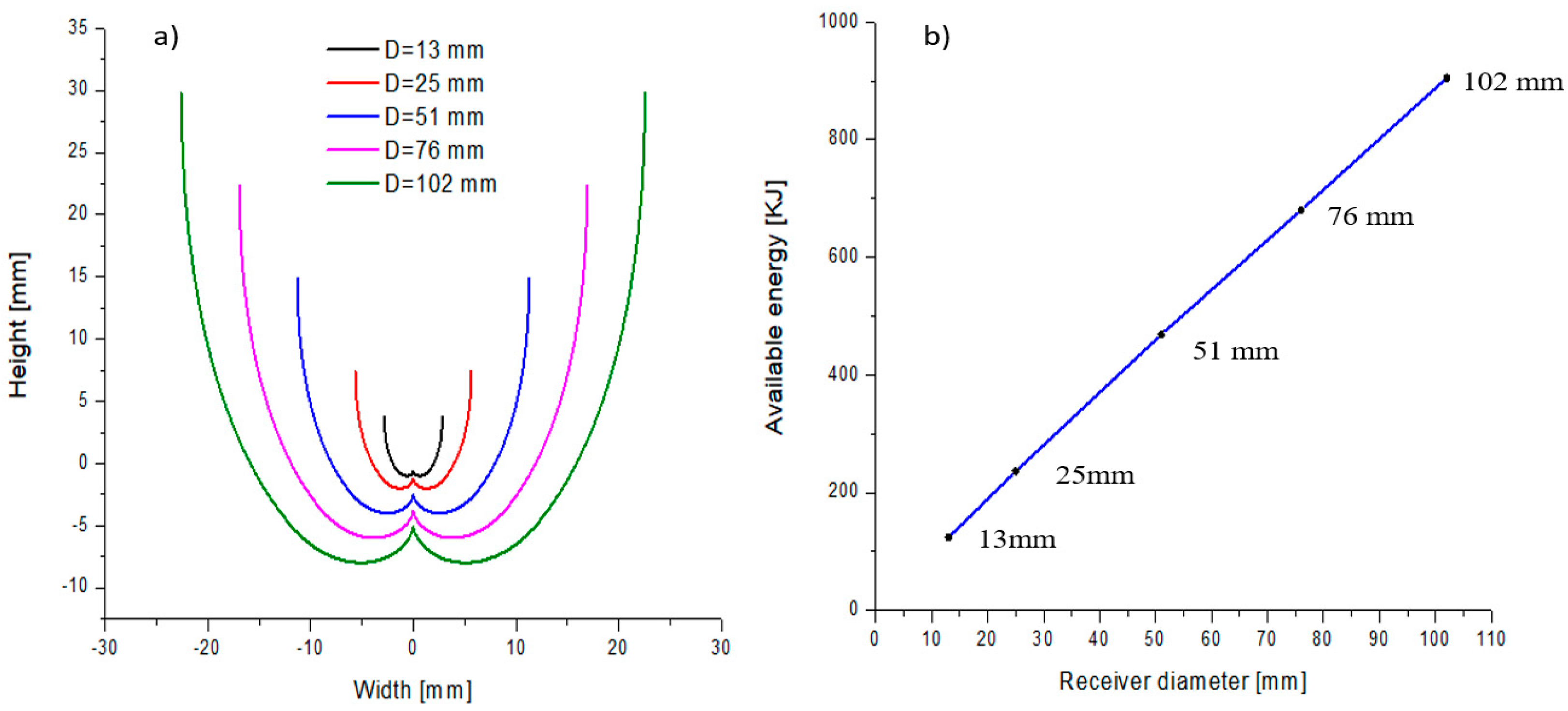
Figure 1a presents an evaluation of the CPC profiles calculated for nominal commercial copper tubing of 13, 25, 51, and 102 mm and their dimensions to aid in the selection of the best concentrator. From these profiles, and taking one meter as the tube length for this study, virtual models were created with Tonatiuh software (open source software 2.2.2, University of Texas, Brownsville, TX, USA) to obtain the available energy in each receiver; the results are shown in Figure 1b. Here, a 13 mm tube was selected as reference, as this is the nominal size of common residential installations. The graph shows that for the 25 mm tube, there would be twice the available energy compared to the 13 mm diameter, which is congruent since the area exposed to the sun’s energy increases in the same proportion, applying the same correspondence for other diameters.
In order to select the receiver diameter, and for comparison purposes, the volume of a commercial flat plate solar heater of 1 m2 was taken as a reference, which has 10 copper tubes of 13 mm in diameter and a volume capacity of 2.17 L. In order to have similar volume capacity in a length of 1 m, a tube with an internal diameter of 51 mm was chosen. This allows simplifying the hydraulic system, which generates a reduction of time and effort in the manufacturing stage.

2.2. Concentrator Design

The concentrator is composed of two identical curved reflecting surfaces placed in such a way that both surfaces are oppositely reflecting a focal point [1,5,23,25,26,27]; in 2004, Chaves provided the appropriate description for the design which uses a cylindrical receiver, contemplating the total illumination of the receiver [26].
Equations for the CPC profile in the Cartesian plane were described by different authors [1,5,23]; however, the equations applicable to this study were described by González et al. [28], projecting the profile of the concentrator from the external diameter of the tubular receiver. The profile is composed of two parts with their respective governing equations. The first part is the bottom profile denominated the involute; the second part at the top is the cup. These equations are evaluated at the lower and upper limits which allow the identification of the points of intersection between the involute and the lower part of the cup. The upper limit sets the maximum width of the cup, which consequently determines the concentrator height. The idea is based on taking advantage of the geometric principle of focusing two curves that shape the cup, which match with the receiver at a certain angle at opposite ends, as well as at the bottom (involute), receiving the solar rays and redirecting them to the receiver. The equations used and their limits for the profile design are as follows.
Involute:
x t = r ( cos θ + θ sin θ )
y t = r ( sin θ + θ cos θ )
Evaluated between the limits of [ π 2 θ a   to   π 2 + θ a ]
Cup:
x = ( sin θ a cos ( θ θ a ) π 2 + θ a + θ cos θ 1 + sin ( θ θ a ) + cos θ a ) r
y = ( cos θ a cos ( θ θ a ) + sin θ a π 2 + θ a + θ 1 + sin ( θ θ a ) sin θ a ) r
Evaluated between the limits of [ π θ a   to   π 2 θ a ] [ π 2 + θ a   to   π + θ a ]
where:
  • θ a = acceptance angle,
  • r = external receiver radius.
For the present study, Equations (1)–(4) with their respective evaluation limits, and the receiver diameter, were used to determine the width and height of the concentrator.

2.3. Virtual Model

A virtual model was generated using Tonatiuh software, taking into consideration characteristic materials available in the market for its construction. The model was positioned in the coordinates (21.02° N, −89.63° W) of the city of Merida, Mexico and it was oriented in the direction of the solar path, i.e., along the east–west direction, tilted to the south at angle β. The present system intends to occupy as little space as possible with low weight, considering its utilization in low- to medium-income residential areas. One alternative optimization is to explore a few adjustments of the concentrator with the inclination angle β, according to the season of the year, the aim being to increase energy availability; therefore, it was necessary to determine the relationship (Sn-θz) of solar angle. Table 1 shows the values of the Sn-θz as a function of the months of the year for Merida, and the corresponding recommended value of the inclination angle (β) of the collector, which applies to any angle of acceptance between −4.27° and 42.16°, thus valid for the proposed coordinates.
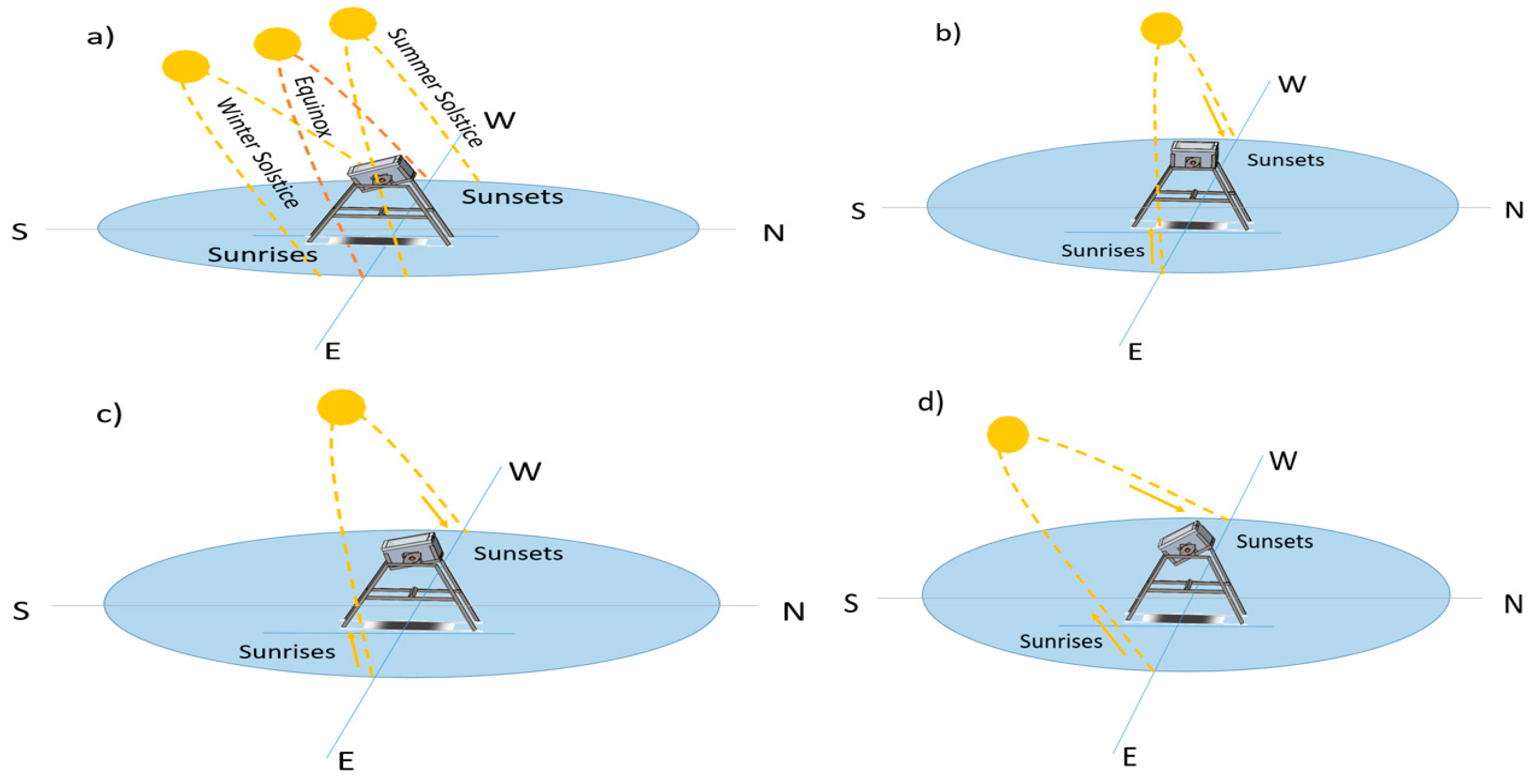
Two cases were analyzed here; static and multi-position setups. For the first case, the inclination angle β throughout the year of the CPC is equal to the present latitude of Merida city, 21° (with respect to the horizontal), as represented in Figure 2a. With the information provided in Table 1, three angles of inclination were selected for the multi-position setup: 0° for summer, 16° for autumn/spring, and 32° for winter, as represented in Figure 2b–d, all tilted anticlockwise with respect to east view. This involves four adjustments a year in three different angular positions. With these data, an analysis campaign was carried out, with the respective seasonal tilted adjustment.
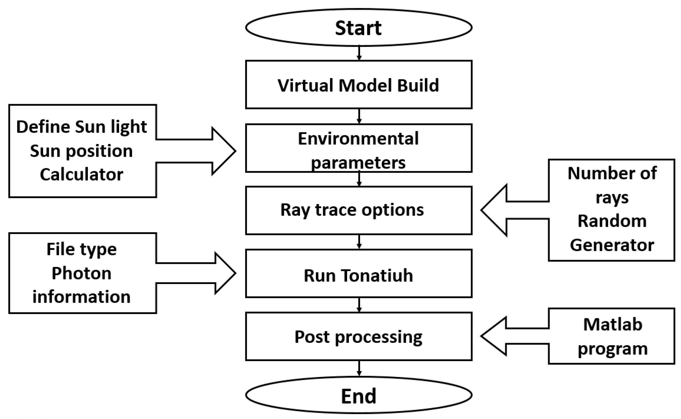
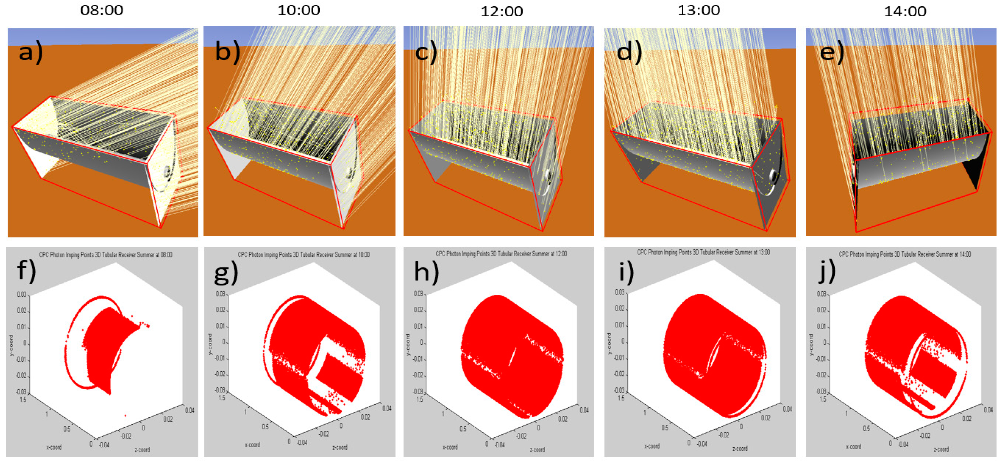
The ray tracing evaluation period was carried out from 8 to 17 h local time. A flowchart of the analysis is shown in Figure 3. From the determination of the concentration ratio (CR) and external diameter of the selected tube, the virtual model is generated, assigning the concentrator and receiver optical properties; subsequently, the environmental parameters are adjusted, which indicate the sun shape, time, and date, for the following random generator and the number of rays. Then we set the receiver type as the target, and the data is stored for further processing with mathematical algorithm software.
Tonatiuh ray tracing software has a fixed sunshape, with the shape of the sun being understood as the variation in the radial energy distribution of the sun derived from its consideration as a non-point light source. There are two techniques to evaluate this: Pillbox and Buie, both were evaluated using the same weather conditions (season, radiation, and time value). The results obtained are shown in Table 2, where values in Pillbox are slightly higher than in Buie, with the highest difference corresponding to spring with 9.36 kJ (0.31%) and the lowest difference corresponding to autumn with 3.39 kJ (0.11%), indicating that no significant differences were found. Further analysis was conducted with the multi-position setup in order to prove the similarity response, finding an agreement in all cases.
Since both techniques gave similar results, for this study the Pillbox sunshape was chosen due to the simplicity of its process. Although Tonatiuh software used here has the capability to carry out a complete analysis with irradiation variations, in this work we are using a fixed irradiation value of 1000 W/m2 as a constant, to simplify the analysis and concentrate on the comparative evaluation of the optical design and the variables such as the influence of the orientation angle throughout the year, in order to evaluate the feasibility for the system to be fixed in a static position or if this requires angle adjustments throughout the year. The importance of this comparative study is to determine whether the CPC could perform satisfactorily in a fixed position throughout the year (or need periodical adjustments), which could make it more attractive for its implementation (in static position). In all cases, the equinoxes of spring and autumn are taken into account, as well as the summer and winter solstices. Since the highest and lowest apparent positions of the sun in the sky are reached in the solstice, the maximum is in summer with the angle of −4.27° and the lowest in winter with the angle of 42.16°, both with respect to the vertical; subsequently, the location coordinates were considered. This allows us to calculate the angular parameters, azimuth, and elevation angle in the study. In order to obtain a confidence level of 97%, according to Blanco [29], a ray tracing of 1,000,000 rays was chosen for the analysis.
Data generated from the ray trace software requires the designing of a post-processing algorithm for data analysis. A MATLAB (R2016a, MathWorks, Natick, MA, USA) algorithm was designed to identify data from sun photons and to classify them as primary, secondary (by rebound), tertiary, etc., in order to provide numerical values (ID, coordinates, power per photon, etc.) and the location of photon impact on the receiver.

2.4. Optical Modeling

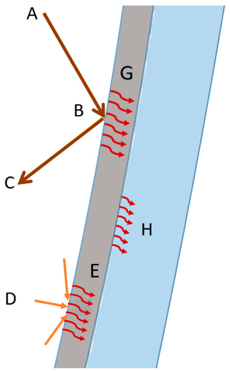
The importance of the optical analysis lies in the fact that it provides information regarding the available energy at the receiver. The input energy was determined using the ray tracing tool and evaluating the energy distribution by incident beam radiation on the collector surface, as represented in Figure 4. The beam radiation follows the path A, B, C, where A and C comply with Fresnel’s law, and B is the energy absorbed by the concentrator. If the angle and energy value of the photon coming from the sun are known (in addition to specular properties of the concentrator), we can determine the path that it follows, impinging the receiver or leaving it out, thereby determining the energy that the receiver reaches.
If the diffuse radiation is taken into account, it is important to consider that the energy and impact angle of a photon is difficult to estimate, since the path depends on the particles present in the atmosphere with which it may impact (dust, water steam, and aerosol), therefore the trajectory and the energy can be affected by the constantly changing environmental composition, making it difficult for the program to predict the amount of diffuse energy aligned to the receivers direction. It is important to consider that diffuse radiation can contribute up to 50% of the energy available in a CPC with a concentration ratio of one (CR = 1), particularly on cloudy days. This study is based on clear skies, where diffuse radiation is low compared to beam radiation and a value of CR equal to 1.41, which minimizes its contribution. Also, given that the objective of this system is to heat water for residential use, beam radiation is way more effective.
In the same Figure 4, D represents the diffuse trajectory, with different energy path and angle of incidence in comparison with A. In the same way, E is the diffuse energy absorbed by the concentrator, G represents the beam energy absorbed by the concentrator, and H is the energy transferred from the concentrator to the insulation material [30].
To determine the available energy at the receiver, a virtual model is proposed which takes into account the properties of the materials (concentrator, receiver, covers) as well as dimensions, system configuration, position of the sun, and the amount of available solar irradiation.
For this study, the following assumptions were made:
(1)
The CPC geometric concentration ratio (CR) is expressed using the formula used by Hsieh [31]:
C R = 1 sin θ a
(2)
The system is considered to be free of manufacturing errors.
(3)
The physical and optical properties of the materials are assumed to be temperature independent.
(4)
The geographical coordinates correspond to the city of Merida, Mexico (21.0291° N, 89.6381° W).
Once the virtual model is implemented, with the characteristics of sun and materials introduced, the energy availability at receiver can be obtained.

2.5. Ray Tracing Analysis

The ray tracing software is based on the Monte Carlo method. It uses the principles of geometric optics, as well as a statistical method that simulates the behavior of a solar concentration system, by generating rays from a simulated source and observing the interactions between the rays and the surfaces of the system. It is conceived as a useful tool in the design and analysis of solar concentration systems [32].
For the analysis, it is assumed that the ray trajectory equals the angle of incidence and the reflected radiation (R); that is, they comply with the Fresnel law. In this sense, the spectral reflectance depends on the reflective material with its refractive index. Before proceeding, it was necessary to determine the incidence angle of the rays (I); this angle is formed between the normal surface (N) and the incident radiation. In order to establish the ray tracing model, the following equation of reflected radiation is used [33]:
R = I 2 ( N · I ) N
To facilitate the analysis, this is decomposed into Cartesian coordinates, applying the following equations:
x R =   sin θ i 2 ( cos θ i cos N + sin θ i sin N ) cos N
y R =   sin θ i 2 ( cos θ i cos N + sin θ i sin N ) cos N
where:
  • N = normal angle of the reflective surface with respect to the coordinate system.
The incident angle for reflected radiation can be determined by:
y R =   sin θ i 2 ( cos θ i cos N + sin θ i sin N ) cos N
In practice, real surfaces are far from ideal; they are related to solar wavelength λ and incidence angle θi (specular reflection). The specular reflection is subjected in the same way to Fresnel’s law; which can be determined by the following equation [33]:
ρ ( θ i , λ ) = ( ρ + ρ ) 2
where ρ and ρ , refers to the perpendicular and parallel reflectivity, determined by the following equations:
ρ =   α 2 + β 2 2 α cos θ i + cos 2 θ i α 2 + β 2 + 2 α cos θ i + cos 2 θ i
ρ = α 2 + β 2 2 α cos θ i tan θ i + sin 2 θ i tan 2   θ i α 2 + β 2 + 2 α cos θ i tan θ i + sin 2 θ i tan 2   θ i

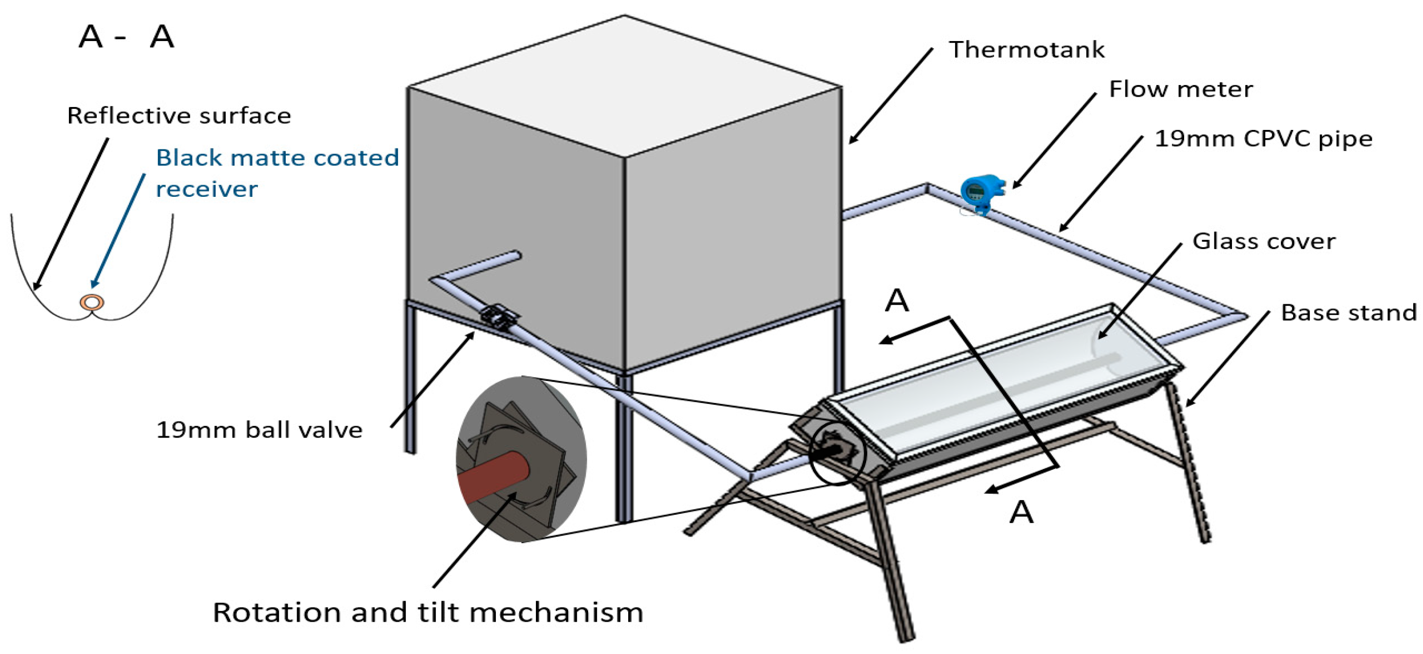
2.6. Experimental Evaluation

The proposed prototype was constructed to evaluate its feasibility, which is represented in Figure 5. The system uses a heat isolated metallic box (with polyurethane) to support and hold the receiver tube; the walls of the box also help to avoid heat exchange between the receiver and the ambient. In addition, a commercial 4 mm thick, flat glass cover was placed on top to reduce convective heat losses to the environment, and mainly due to the influence of constant air currents.
The concentrator was designed with 95% high reflectance aluminum (specular reflectivity), according to the American Standard Test Methods; ASTM STP478 (Specular and Diffuse Reflectance Measurements of Aluminum Surfaces), where the incident ray on this surface is reflected at the same angle of incidence with respect to the normal surface. The values of the optical properties of the materials are shown in Table 3.
Thermal efficiency for the experimental evaluation was obtained using the following equation:
η = m ˙ c p ( T o u t l e t T i n l e t ) A c o v   I   d t
In order to speed up the thermosiphon effect and reduce the scale accumulation in the receiver wall (at higher temperatures), which interferes with the heat transfer process and, in consequence, reduces the efficiency; a 3 W submersible solar pump was installed in the system, which provides a maximum flow of 0.05 L/s, reporting this way, a ∆T of 7 °C between inlet and outlet of receiver. For these conditions, if the internal diameter is reduced, the flow velocity of the fluid used, increases, which directly results in a reduction in the temperature difference between inlet and outlet. On the other hand, if the diameter increases, the material and therefore the cost, also increases. Consequently, it was decided to evaluate a CPC using a copper receiver with 54 mm external diameter (51 mm internal diameter), coated with matte, non-selective, high-temperature black paint.
A complete CPC was constructed using the following dimensional parameters: 0.24 m aperture width, 0.19 m height and 1 m length, with an acceptance angle of 45°, which correspond to a concentration ratio of 1.41 [31]. The theoretical temperature of the thermodynamic limit for this concentration ratio is 156.5 °C [34]. However, this presents some challenges to take into account; the manufacture of a complex involute and cup profile, with a high reflective material (thin sheet of aluminum) high cost of materials and greater energy demand for heating the fluid due to volume increase.

3. Results and Discussion

3.1. Static Position Setup

The results of the CPC’s ray trace campaign, positioned at 21° (as the static arrangement), are shown in Table 4. The values are grouped in columns corresponding to the seasons of the year, and the rows to a progressive timeline at every hour from 8 to 17 h. The analysis shows the amount of energy gathered, represented by photon dots impinging on the receiver, where each photon is counted with an energy value depending on the previous rebound made, direct from the sun and those that impacted first on the reflective surface of the concentrator, one or more times, before reaching the receiver. Although the analysis shows visually the amount of photons that impinge on the receiver, it is difficult to estimate the total energy accumulated by each photon impact, since the energy of each photon is path dependent; that is, if it directly impacts the receiver, it will take all the energy available, where the coordinates of this photon are recorded accordingly. In the case where the photon impacts first on the concentrator (reflecting surface), it loses some energy due to the reflectivity coefficient of the surface [12]. This tracking procedure is carried out individually with the aid of a MATLAB protocol, to ease the energy quantification by photon counting [29].
Table 4 shows the complete energy availability gathered with the ray trace software. The table shows the total energy produced by photon impacts incident on the receiver for each season. As can be seen, autumn and spring present greater availability of energy, while winter and summer are around 11.88% below those seasons. The total energy available from the interaction of the photons for each season resulted in an annual average of 2824 kJ.
Another interesting fact observed is that in winter and summer, there is a total of three hours in which the incidence of photons is very low (values less than 130 kJ). This is due to the effect of the concentrator lateral walls and the relative position of the sun in the celestial vault. Figure 6 shows the virtual model with a visual representation of these cases, evaluated in summer. To provide further information on the effect of shading by the lateral walls, the ray tracing evolution through the subsections is plotted. In Figure 6a,f, it is noticeable that at 8 h, rays impact the lateral wall and an external part of the CPC concentrator (non-reflecting surface). Photons that impact the concentrator on the reflecting surface are rebound and reach the receiver, although some of them go from one side to another of the concentrator until they leave this without impinging on the receiver. This is due to the photons having an angle of incidence which is greater than 47° with respect to the horizontal. The non-impacted area of the receiver is shown as white segments. Figure 6b,g shows how the shading effect decreases and the impacts on the receiver increase. Direct impacts occur on the top of the receiver due to the sun’s direct rays and on the sides and bottom parts of the system due to reflection from the concentrator, which contribute to the sum of the energy. Figure 6c,h shows that at 12 h, the number of photon impacts are still increasing. The maximum impact of photons occurs at around 13 h, which corresponds to solar noon, in which practically all of the top receiver is directly impacted by photons, as shown in Figure 6d,i. Finally, Figure 6e,j gives information from 14 h, where the photon impacts decrease again, partly due to the influence of the lateral walls that once again begin to block the path of the photons. Since there is a symmetrical behavior, there will be another two hours in which shading is produced in the concentrator on the left side towards the sunset.
Figure 7 shows a graph for the analyses of the responses from the four seasons, in static setup (at 21°). The highest concentration of energy in the day is located in spring with 2995 kJ, while the lowest energy registered is in winter with 2677 kJ, 10.62% less than the first one. The availability of energy in autumn is 2946 kJ, 1.65% less than spring, and summer is 2678 kJ, 10.59% less than spring too. On comparing spring versus autumn and summer versus winter, small differences of 1.65% and 0.035%, respectively, can be observed. A detailed inspection of Figure 7 shows that there are two types of curve patterns: one for the spring and winter seasons and another for autumn and summer, where the total energy under the curve between each pair of similar graphs resulted in similar energy values. A comparison of the energy curves shows a modest decrease in energy caption, suggesting the feasibility of implementing a solar heater in a static setup, since only around 11% of energy will be unavailable for the winter and summer seasons in comparison with the autumn and spring seasons.

3.2. Multi-Position Setup

The results of the evaluation of energy distribution in the receiver in a multi-position setup are shown in Table 5. The evaluation was carried out for the same time span (from 8 to 17 h). The adjustments of the system were implemented following the angle distribution of Table 1 (summer 0°, spring/autumn 16°, winter 32°), see representation in Figure 5. After carrying out the data processing routine, energy availability information was gathered, shown in Table 5. It is noticeable that the greatest energy availability occurs in autumn and spring and the least favored season is once again winter. The highest energy concentration in the day is located in autumn with 3860 kJ, while the lowest energy is registered in winter with 3370 kJ, that is, 12.70% of difference between them. The total energy available from the interaction of the photons for each season resulted in an annual average of 3587 kJ.
Figure 8 shows a graph for the analysis of the responses from the four seasons, evaluated in multi-position setup. The energy availability in spring is 3641 kJ, 5.68% less than autumn, the highest total energy recorded (3860 kJ), whereas in summer it is 3477 kJ, 9.93%, less than autumn, too. Interestingly, on comparing summer versus winter, a difference of only 3.07% can be observed. A detailed inspection of Figure 8 shows that there are similarities in the curve patterns, where the total energy under curves, resulted in higher energy values in comparison with static setup. The comparison of the energy curves shows a slight decrease in energy caption between the most energetic (autumn) and the least energetic (winter), where, in the case of multi-position setup, the biggest difference between seasons, resulted in an energy difference of around 13%. This resulted in a more attractive option to implement as a solar heater (multi-position setup) in comparison with the static setup. The highest energy values available for these curves, were observed at around 13 h, corresponding to the solar noon.
A data comparison of the static setup (Table 4) and the multi-position setup (Table 5), showed important differences; where the energy available for autumn in the multi-position setup (16°) is 3860 kJ, while at 21° it resulted in 2946 kJ, giving an energy gain of 31.12% for the first one. For winter at 32°, the orientation angle in the multi-position setup reached 3370 kJ, compared with its static setup counterpart (at 21°) of 2677 kJ, this being equivalent to a 25.87% energy gain (for multi-position setup).
Similarly, for spring, the multi-position setup at 16° achieved 3651 kJ, while the static setup was as low as 2995 kJ, representing a 21.91% energy gain. Finally, it was determined that for summer, in the multi-position setup of 0°, an energy availability of 3509 kJ was gathered, while for the static setup, there was an energy availability of 2678 kJ, equivalent to a 31.03% energy gain (for multi-position setup). In general, an average annual energy of 3587 kJ was obtained for the multi-position setup, which corresponds to a gain of 22% with respect to the average annual obtained in static setup (2824 kJ).
Complementary to the analysis, the photons impinging on the receiver was evaluated with only the two less energetic seasons (winter and summer), although the analysis was carried out for the four seasons. Figure 9 shows a comparison of these two seasons, as the other two (autumn and spring) resulted visually very similar; therefore, it was decided to analyze and show the least energetic ones. Here, the seasons are shown in two modalities; 21° corresponding to static setup (SS) and 32° and 0° corresponding to multi-position setup (MS) for winter and summer, respectively. For multi-position setup, winter and summer show similarities in the amount of photon impacts achieved, observed visually (formation of the cylindrical profile), in comparison with the static setup seasons at 21° (winter and summer), where fewer photon impacts can be appreciated, confirming that more energy capture can be gather with the multi-position setup.

3.3. Experimental Analysis for Static Setup

A prototype was built and tested in order to verify that the proposed system adjusts to residential-level temperatures in real conditions. According to Duffie et al. [5], low concentration systems with a concentration ratio (CR) between 1 and 3, take advantage of both diffuse and beam radiation in similar proportions. The present system in study has a CR = 1.41, therefore, the contribution of beam and diffuse radiation is considered in this application.
Using the proposed system (Figure 5) and the information provided by the Meteonorm climatological station located in Merida [35], Figure 10 shows the solar radiation/flow vs. time, and flow/temperature vs. time on a specific winter day (29 December 2016).
Figure 10a shows the global beam and diffuse radiation, as well as flow vs. time, where it can be seen that global radiation starts practically from zero at 7 h. Between 7 and 12 h a continuing increase of global radiation is observed, reaching its maximum between 12 and 13 h, and then gradually decreasing until it reaches practically 0 global radiation at 18 h; which is consistent with the radiation distribution of a typical solar day.
Figure 10b shows the variations in ambient temperature, as well as inlet and outlet fluid temperature in the receiver during working hours (8 to17 h) of the same day (29 December 2016). It can be observed that the increase in the outlet temperature is a result of the increase of global radiation, up to a point where the outlet temperature suddenly decreases at 9 h; which is related to the activation of the submersible pump controlled by a thermostat that kept working from 9 to 17 h. An hour later (10 h), it can be seen that the outlet temperature recovers due to the increase in diffuse radiation. This radiation–temperature increase relationship continues until 13 h. Similarly, when the radiation starts to decrease (Figure 10a), the outlet temperature follows the same behavior (Figure 10b).
The overall heating energy obtained during the present experiment reached 1800 kJ (29 December 2016), with an efficiency of around 42.98% (using Equation (13)). This modest efficiency is attributed to the limited incident energy that was transferred to the receiver, as well as the inherent CPC prototype design, with the materials used and quality of manufacture of the system, as well as the type of paint used on the receiver and manufacturing defects of the concentrator. With this experimental evaluation, it was proven that the proposed system is capable to work at residential temperature range, even though further work is required in order to improve the abovementioned characteristics of the system to increase its efficiency.

4. Conclusions

This paper presents a prediction tool to analyze the energy performance of a CPC system under different working conditions over a seasonal year. Here, setups in two modalities were evaluated: stationary and multi-position. The analysis was performed using a ray tracing software and a mathematical algorithm software for data processing. The tool proved to be useful to estimate the maximum theoretical energy present in the solar collector, to study the relevant optical–structural response and to determine the strength and weakness of a prototype before its construction. Adverse conditions such as winter can be predicted, and adjustments can be made to adequate the CPC design prior to its construction. The annual energy distribution in the receiver was analyzed, and it proved to be useful for predicting the energy availability, allowing the implementation and use of strategies to reduce heat losses, based on the ideal conditions.
From this study, with the data provided theoretically, it was possible to determine that, with the use of the multi-position setup of the CPC throughout the year, the energy availability was 22% more than the static setup, resulting in a more attractive alternative. Therefore, the multi-position setup can be taken into consideration as part of a further study for an improved system construction and its validation.
Complementary to the theoretical analysis, an implementation and evaluation of a CPC was carried out. With the experimental test conducted, it was proven that it is possible to obtain temperatures corresponding to residential use with a CPC of reduced dimensions, thus providing feasibility, when compared to other collectors such as FPH—an option with reduced materials and possible reduced manufacturing time and costs, too. Further works are needed for technical improvements.

Acknowledgments

This work was supported by the project SENER-CONACYT S0019-2014-01, grant number 254667 and the project PDCPN-CONACYT, grant number 2015-01-1651.

Author Contributions

Miguel Terrón-Hernández and Jose G. Carrillo conceived the paper and drafted it; Miguel Terrón-Hernández, Manuel I. Peña-Cruz, performed the ray trace analysis; Miguel Terrón-Hernández and Ulises Diego-Ayala built and instrumented the CPC; Miguel Terrón-Hernández and Vicente Flores performed the thermal analysis.

Conflicts of Interest

The authors declare no conflict of interest.

Nomenclature

θ Parametric angle for involute [rad]
θ a Acceptance angle [rad]
r External receiver radius [m]
r Radius of absorber [m]
CRGeometric concentration ratio [-]
RReflected radiation [W/ m 2 ]
ISolar irradiance [W/ m 2 ]
θ i Incident angle [rad]
N Normal angle of the reflective surface with respect to the coordinate system [-]
θ R Incident angle for reflected radiation [rad]
x R Coordinate axis x for reflected radiation
y R Coordinate axis y for reflected radiation
A c o v Cover area [m2]
ρ Parallel reflectivity [-]
ρ Perpendicular reflectivity [-]
C p Specific heat [J kg−1 K−1]
m ˙ Mass flow rate [kg s−1]
T i n l e t Inlet fluid temperature [K]
T o u t l e t Outlet fluid temperature [K]
d t Differential of time [h]
λSolar wavelength
ρReflectance
Absorptance
βTilted angle
ηThermal efficiency

References

  1. Winston, R.; Miñano, J.C.; Benitez, P. Nonimaging Optics; Academic Press: San Diego, CA, USA, 2005; pp. 50–63. ISBN 0-12-759751-4. [Google Scholar]
  2. Kalogirou, S.A. The potential of solar industrial process heat applications. Appl. Energy 2003, 76, 337–361. [Google Scholar] [CrossRef]
  3. Kalogirou, S.A. Design and construction of a one-axis sun-tracking system. Sol. Energy 1996, 57, 465–469. [Google Scholar] [CrossRef]
  4. Rabl, A. Comparison of Solar Concentrators. Sol. Energy 1976, 18, 93–111. [Google Scholar] [CrossRef]
  5. Duffie, J.A.; Beckman, W.A. Solar Engineering of Thermal Processes, 4th ed.; John Wiley & Sons: Hoboken, NJ, USA, 2013; pp. 337–342. ISBN 978-0-470-87366-3. [Google Scholar]
  6. Gaos, Y.S.; Yulianto, M.; Juarsa, M.; Nurrohman; Marzuki, E.; Yuliaji, D.; Budiono, K. The performance of solar collector CPC (compound parabolic concentrator) type with three pipes covered by glass tubes. AIP Conf. Proc. 2017, 1826, 020022. [Google Scholar] [CrossRef]
  7. Wang, Q.; Wang, J.; Tang, R. Design and Optical Performance of Compound Parabolic Solar Concentrators with Evacuated Tube as Receivers. Energies 2016, 9, 795. [Google Scholar] [CrossRef]
  8. Yurchenko, V.; Yurchenko, E.; Ciydem, M.; Totuk, O. Ray tracing for optimization of compound parabolic concentrators for solar collectors of enclosed design. Turk. J. Electr. Eng. Comput. Sci. 2015, 23, 1761–1768. [Google Scholar] [CrossRef]
  9. Singh, H.; Eames, P. Correlations for natural convective heat exchange in CPC solar collector cavities determined from experimental measurements. Sol. Energy 2012, 86, 2443–2457. [Google Scholar] [CrossRef]
  10. Tchinda, R. Thermal behaviour of solar air heater with compound parabolic concentrator. Energy Convers. Manag. 2008, 49, 529–540. [Google Scholar] [CrossRef]
  11. Horta, P.; Osório, T.; Collares-Pereira, M. Energy cost based design optimization method for medium temperature CPC collectors. AIP Conf. Proc. 2016, 1734, 020011. [Google Scholar] [CrossRef]
  12. Häberle, A.; Apian-Bennewitz, P.; Schmidt, T.; Troescher, T.; Wittwer, V. Amount of solar radiation absorbed by trough collectors with nonimaging optics. In Optical Materials Technology for Energy Efficiency and Solar Energy Conversion XIII; International Society for Optics and Photonics: Freiburg, Germany, 1994. [Google Scholar] [CrossRef]
  13. Widyolar, B.; Jiang, L.; Winston, R. Thermodynamics and the segmented compound parabolic concentrator. J. Photonics Energy 2017, 7, 028002. [Google Scholar] [CrossRef]
  14. Lovegrove, K.; Stein, W. Concentrating Solar Power Technology: Principles, Developments and Applications; Woodhead Publishing Limited: Sawston, UK, 2012; pp. 26–33. ISBN 978-1-84569-769-3. [Google Scholar]
  15. Winter, C.; Sizmann, R.; Vant-Hull, L. Solar Power Plants: Fundamentals, Technology, System, Economics; Springer: Berlín, Germany, 1991; pp. 41–53. ISBN 978-3-642-64759-8. [Google Scholar]
  16. Arancibia-Bulnes, C.A.; Peña-Cruz, M.I.; Mutuberría, A.; Díaz-Uribe, R.; Sánchez-González, M. A survey of methods for the evaluation of reflective solar concentrator optics. Renew. Sustain. Energy Rev. 2017, 69, 673–684. [Google Scholar] [CrossRef]
  17. Suresh, D.; O’Gallagher, J.; Winston, R. Thermal and optical performance test results for compound parabolic concentrators (CPCs). Sol. Energy 1990, 44, 257–270. [Google Scholar] [CrossRef]
  18. Ustaoglu, A.; Okajima, J.; Zhang, X.-R.; Maruyama, S. Evaluation of the efficiency of dual compound parabolic and involute concentrator. Energy Sustain. Dev. 2016, 32, 1–13. [Google Scholar] [CrossRef]
  19. Colina-Marquez, J.A.; Lopez-Vasquez, A.F.; Machuca-Martinez, F. Modeling of direct solar radiation in a compound parabolic collector (CPC) with the ray tracing technique. Dyna 2010, 77, 132–140. [Google Scholar]
  20. Kuo, C.-W.; Yen, P.-S.; Chang, W.-C.; Chang, K.-C. The Design and Optical Analysis of Compound Parabolic Collector. Procedia Eng. 2014, 79, 258–262. [Google Scholar] [CrossRef]
  21. Waghmare, S.A.; Gulhane, N.P. Design and ray tracing of a compound parabolic collector with tubular receiver. Sol. Energy 2016, 137, 165–172. [Google Scholar] [CrossRef]
  22. Chen, L.; Chen, J.-X.; Zhang, X.-R. Numerical simulation on the optical and thermal performance of a modified integrated compound parabolic solar concentrator. Int. J. Energy Res. 2015, 39, 1843–1857. [Google Scholar] [CrossRef]
  23. Bellos, E.; Korres, D.; Tzivanidis, C.; Antonopoulos, K.A. Design, simulation and optimization of a compound parabolic collector. Sustain. Energy Technol. Assess. 2016, 16, 53–63. [Google Scholar] [CrossRef]
  24. Osorio, T.; Horta, P.; Larcher, M.; Pujol-Nadal, R.; Hertel, J.; van Rooyen, D.W.; Heimsath, A.; Schneider, S.; Benitez, D.; Frein, A.; et al. Ray-tracing software comparison for linear focusing solar collectors. AIP Conf. Proc. 2016, 1734, 020017. [Google Scholar] [CrossRef]
  25. Pei, G.; Li, G.; Zhou, X.; Ji, J.; Su, Y. Experimental study and exergetic analysis of a CPC-type solar water heater system using higher-temperature circulation in winter. Sol. Energy 2012, 86, 1280–1286. [Google Scholar] [CrossRef]
  26. Chaves, J. Introduction to Nonimaging Optics; CRC Press: Madrid, Spain, 2008; pp. 10–23, 25–35. ISBN 978-1-4200-5429-3. [Google Scholar]
  27. Abdullahi, B.; Al-Dadah, R.K.; Mahmoud, S.; Hood, R. Optical and thermal performance of double receiver compound parabolic concentrator. Appl. Energy 2015, 159, 1–10. [Google Scholar] [CrossRef]
  28. González, M.E.; Rincón, M.E.A.; Moreno, L.D. Using a new solar sterilizer for surgical instruments as a solar oven for cooking. In Proceedings of the VIII Congreso Ibérico, VI Congreso Iberoamericano de las Ciencias y Técnicas del Frío (CYTEF 2016), Coimbra, Portugal, 3–6 May 2016. [Google Scholar]
  29. Blanco, M.; Mutuberria, A.; Monreal, A.; Albert, R. Results of the empirical validation of Tonatiuh at Mini-Pegase CNRS-PROMES facility. In Proceedings of the SolarPACES (2011), Granada, Spain, 20–23 September 2011. [Google Scholar]
  30. Eames, P.C.; Norton, B. Validated Unified Model for optics and heat transfer in line-Axis concentrating solar energy collectors. Sol. Energy 1993, 50, 339–355. [Google Scholar] [CrossRef]
  31. Hsieh, C.K. Thermal analysis of CPC collectors. Sol. Energy 1981, 27, 19–29. [Google Scholar] [CrossRef]
  32. Giovinazzo, C.; Bonfiglio, L.; Gomes, J.; Karlsson, B. Ray Tracing Modelling of an Asymmetric Concentrating PVT. In Proceedings of the Eurosun 2014, Aix-les-Bains, France, 16–19 September 2014. [Google Scholar]
  33. Ustaoglu, A.; Alptekin, M.; Okajima, J.; Maruyama, S. Evaluation of uniformity of solar illumination on the receiver of compound parabolic concentrator (CPC). Sol. Energy 2016, 132, 150–164. [Google Scholar] [CrossRef]
  34. Goswami, D.Y.; Kreith, F.; Kreider, J.F. Principles of Solar Engineering, 3rd ed.; CRC Press: Boca Raton, FL, USA, 2000; pp. 164–167. ISBN 978-1-4665-6379-7. [Google Scholar]
  35. Meteotest. Available online: http://www.meteonorm.com/ (accessed on 10 February 2017).
Figure 1. (a) 13, 25, 51, and 102 mm, nominal diameters of Compound Parabolic Concentrator (CPC) profiles; (b) Available energy vs. receiver diameter.
Energies 11 00291 g001
Figure 2. Representation of CPC tilting (a) Static setup 21°; (b) summer 0°; (c) spring/autumn 16°; and (d) winter 32°.
Energies 11 00291 g002
Figure 3. CPC flowchart methodology.
Energies 11 00291 g003
Figure 4. Representative energy diagram in the concentrator.
Energies 11 00291 g004
Figure 5. CPC prototype for the present study.
Energies 11 00291 g005
Figure 6. Evolution of (ae) shading and (fj) photon impacts on the receiver for summer solstice from 8 to 14 h, for a static setup (21°).
Energies 11 00291 g006
Figure 7. Comparison of available energy on receiver per season in static setup (21°).
Energies 11 00291 g007
Figure 8. Available energy at receiver with multi-position setup (summer 0°, spring/autumn 16°, winter 32°).
Energies 11 00291 g008
Figure 9. Photon impacts comparison for winter and summer in static setup (SS, 21°) and multi-position setup (MS, 0° for summer and 32° for winter).
Energies 11 00291 g009
Figure 10. Experimental evaluation of (a) Radiation of Merida Yucatan and (b) ambient, inlet, and outlet CPC temperatures obtained on the 29 December 2016.
Energies 11 00291 g010
Table 1. Merida solar angle (Sn- θ z ).
DateSn-θz (°)β (°)
15 January40.10232
15 February32.1232
15 March21.6516
15 April9.4116
15 May0.0410
15 June−4.270
15 July−2.680
15 August5.0490
15 September16.6116
15 October28.4332
15 November37.9832
15 December42.1632
Table 2. Buie and Pillbox comparative sunshape energy for one specific day.
Local TimeAutumnWinterSpringSummer
BuiePillboxBuiePillboxBuiePillboxBuiePillbox
(h)(kJ)(kJ)(kJ)(kJ)(kJ)(kJ)(kJ)(kJ)
820.1220.99132.51132.15154.58154.731.81.44
9131.9133.03248.47247.97263.34263.39130.53130.03
10262.98265.77349.99350.60348.73348.23224.38224.99
11364.32365.83427.42430.70420.87418.19334.58337.86
12451.44449.96465.8469.69472.5472.64420.08423.97
13480.85479.34407.95410.51421.05418.49474.22476.78
14409.32410.24323.64321.88352.29345.63419.36417.60
15367.48367.52216.18216.43265.03262.89350.56350.81
16301.64301.5197.8896.41188.96187.42224.96223.49
17133.95133.317.667.6198.8296.4997.9597.90
Total2946.062949.452677.52683.932995.483004.842678.432684.86
Table 3. Optical properties of the materials used for the CPC construction.
ElementReflectivityTransmissivityAbsorptivityEmissivity
Concentrator0.870.030.05–0.100.05
Receiver0.0900.910.94
Glass0.070.810.120.92
Table 4. Energy availability on static setup receiver (21°) for annual seasons.
Local Time (h)Autumn (kJ)Winter (kJ)Spring (kJ)Summer (kJ)
820.12132.51154.581.8
9131.90248.47263.34130.53
10262.98349.99348.73224.38
11364.32427.42420.87334.58
12451.44465.80472.5420.08
13480.85407.95421.05474.22
14409.32323.64352.29419.36
15367.48216.18265.03350.56
16301.6497.88188.96224.96
17133.957.6698.8297.95
Total2946.062677.52995.482678.43
Table 5. Seasonal energy availability at receiver for multi-position setup (summer 0°, spring/autumn 16°, winter 32°).
Local Time (h)Autumn (kJ)Winter (kJ)Spring (kJ)Summer (kJ)
8251.14185.97221.60171.79
9380.59289.47359.73277.87
10421.16374.67396.30353.07
11473.78436.35462.38415.98
12479.59475.70481.21463.72
13487.62462.35480.51490.50
14452.34413.57464.40475.16
15409.57338.32380.84385.85
16310.78247.02269.96276.70
17193.57146.63123.91166.29
Total3860.143370.053640.843476.93

